www.ijsrp.org
Construction of Control Chart for Random Queue
Length for (M / M / c): (
/ FCFS) Queueing Model
Using Skewness
Dr.(Mrs.) A.R. Sudamani Ramaswamy
, Mrs. B.Vennila
*Department of Mathematics, Avinashilingam Institute for HomeScience and Higher Education for Women, Coimbatore-43. **Department of Mathematics, Sri Ramakrishna Engineering College, Coimbatore-22.
Dr. (Mrs.) A.R. Sudamani Ramaswamy, Ph.D, [email protected]
Correspondence Author: Mrs. B.Vennila, M.Phil, [email protected]
ABSTRACT
In this paper, first-come, first served, multiple channel Poisson/exponential queueing system M / M / c with infinite waiting capacity is considered. For this model, we introduce a new procedure for construction of
i) Shewhart’s control chart C1,
ii) Control chart C3 for random queue length N using the method on skewness suggested by Shore(2000) and the control
charts C1 and C3 are compared.
Index Terms: Random queue length, Average run length, False alarm rate, Average queue length.
1. INTRODUCTION
Waiting in line for service is one of the most unpleasant
experiences of life on this world. Barrer (1957) says, In certain queueing processes a potential customer is considered “lost” if the system is busy at the time service is demanded. If not served during this time, the customer leaves the system and is considered lost. In queueing system the customer satisfaction can be increased by constructing control charts for N and providing control limits for N so as to make effective utilization of time. If control limits are displayed so that customer can have prior idea about control limits.
With this factor, an attempt is made to find control limits for
random queue length N for (M/M/c) : (∞/FCFS) queueing model. The pioneering work in this direction was made by Haim Shore in 2000. Two control charts C1 and C2 are constructed for random queue length N for (M/M/1) : (∞/FCFS)
www.ijsrp.org
queueing model by Khaparde and Dhabe (2010) and also C3 and C4 are constructed for random queue length N for
(M/M/1) : (∞/FCFS) queueing model by Khaparde and Dhabe (2011) where Control chart C1 : is the Shewhart control chart,
Control chart C2 : is the control chart using method of weighted variance,
Control chart C3 : is the control chart for random queue length N based on skewness and
Control chart C4 : is the control chart using Nelson’s power transformation.
In this paper construction of control chart C3 for random queue
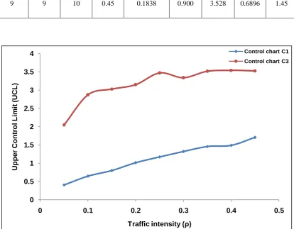
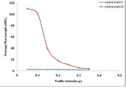
length N for (M/M/c) : (∞/FCFS) queueing model is done using method based on skewness. Performance of control chart C3 is
compared with control chart C1.
2. (M / M / c) : ( / FCFS) QUEUEING MODEL
[image:2.595.35.279.561.695.2]In this model arrival follows Poisson distribution with parameter and service time follows independently and identically distributed exponential distribution with parameter . There are c identical servers present in the system. Figure I represent the state-transition diagram for this model.
FIGURE I : STATE-TRANSITION RATE DIAGRAM FOR M / M / c MODEL
Let random variable N denote the number of customers in the system both waiting and in service and Pn denote the
steady state distribution of random variable N given by
Pn =
c
!
P
,
c
n
c
1
c
n
1
,
P
!
n
1
0 c n c
0 n
(1)
where P0 =
,
c
c
!
c
1
!
n
1
1 1
c
0 n
c
n
is the mean arrival rate and is the mean service rate.
Let random variable WS denote the waiting time spent in the system by the customer. This includes both the waiting time
and service time. The p.d.f. of random variable WS is given by
0
1
1
c
1
c
1
(c
1)
c
c+1
c
c
www.ijsrp.org
f(WS) = ()
e
S,
W ) (
WS > 0 (2)
Thus WS follows an exponential distribution with mean
E(WS) =
0
S S
S
f(W
)
d
W
W
=
0
S W
) (
S
(
)
e
d
W
W
SE(WS) =
)
(
1
(3)
E
(
W
)
2
S = 2
)
(
2
(4)Using (2.3) and (2.4), the variance is given by
V(WS) = 2
)
(
1
(5)The distribution function of WS is
F(x) = P(WS x) =
0
S S
)
d
W
f(W
=
0
S W
) (
W
d
e
)
(
S= 1 e () x, x > 0.
∴ F(x) = 1 e (1 ) x, x > 0.
The probability distribution of N is a geometric distribution with parameter (1 ). The steady state distribution of the random variable N depends on two parameters and only through their ratio.
Using (1), the average number of customers and variance of queue length in the system is given by
E(N) =
1 =
1 c
0 n
n
P
n
+
c
n n
P
n
=
1 c
0 n
n
n
!
n
1
P0 +
c
n
n
n
!
c
c
www.ijsrp.org
= P0
c
c
!
1)
(c
1
!
1)
(n
1
c1 c
0 n
n
Here P0 =
1 c
1 c
0 n
n
c
c
!
c
1
!
n
1
∴ E(N) =
1 =1 c
1 c
0 n
n
c
c
!
c
1
!
n
1
x
c
c
!
c
1
!
n
1
c1 c
0 n
n
(6)
E(N2) =
2 =
0 n
n
n
n
P
)
P
1)
(n(n
=
1 c
0 n
n
P
1)
n(n
+
c n
n
P
1)
c(c
+
1 c
0 n
n
P
n
+
c
n n
P
c
=
1 c
0 n
1)
n(n
n
!
n
1
P0 +
c n
1)
c(c
n
!
c
c
1
c n P0+
1 c
0 n
n
n
!
n
1
P0 +
c
n
c
n
!
c
c
1
c n P0E(N2) =
2 =1 1
c
0 n
c n
c
c
!
c
1
!
n
1
x
1 1
c
0 n
2 c
2 n
!
c
c
c
c
!
n
n
(7)Using (6) and (7), the variance of queue length in the system is given by
V(N) =
1 1
c
0 n
c n
c
c
!
c
1
!
n
1
x
1 1
c
0 n
2 c
2 n
!
c
c
c
c
!
www.ijsrp.org
2 1 c 0 n c nc
c
!
c
1
!
n
1
x
2 1 c 0 n c nc
c
!
1)
(c
1
!
1)
(n
1
(8)Using (8), the standard deviation is calculated as
=
1 c 0 n c n 2 / 1 2 1 c 0 n c n 1 c 0 n 2 c 2 n 1 c 0 n c nc
c
!
c
1
!
n
1
c
c
!
1)
(c
1
!
1)
(n
1
!
c
c
c
c
!
n
n
x
c
c
!
c
1
!
n
1
(9)E(N3) =
3 =
0 n nP
n)
1)
(n
3n
2)
(n
1)
(n(n
= P0
1 c 0 n n!
n
1
2)
(n
1)
n(n
+ c n c c nc
1
!
c
2)
(c
1)
(c
c
+ 3
1 c 0 n n!
n
1
1)
n(n
+ 3
cn n c
n
c
1
!
c
1)
(c
c
+
n c n c
n 1 c 0 n n
c
1
!
c
c
!
n
1
n
3
= 1 c 1 c 0 n nc
c
!
c
1
!
n
1
x
c
!
c
c
c
!
n
n
c 3www.ijsrp.org
Using (10), the third central moment is given by
3 =
c
!
c
c
c
!
n
n
c
c
!
c
1
!
n
1
c 1 c 30 n 3 n 1 c 1 c 0 n n -3
c
!
c
c
c
!
n
n
c
c
!
c
1
!
n
1
c 1 c 20 n 2 n 2 c 1 c 0 n n x
(c
1)
!
1
c
c
!
1)
(n
1
c 1 c 0 n n + 2
3 c 1 c 0 n n!
c
1
c
c
!
n
1
3 = 3
c 1 c 0 n n 2 c 1 c 0 n 2 n c 1 c 0 n n c 1 c 0 n n 3 c 1 c 0 n 3 n 2 c 1 c 0 n n
!
c
1
c
c
!
n
1
!
c
c
c
c
!
n
n
x
!
1)
(c
1
c
c
!
1)
(n
1
x
c
c
!
c
1
!
n
1
3
!
c
c
c
c
!
n
n
c
c
!
c
1
!
n
1
(11) Let Sk(N) denote the traditional measure of skewness for random queue length namely,Sk(N) = 3
3
.
www.ijsrp.org
Using (9) and (11), the skewness for random queue length is given by Sk(N) =
3/2 2 c
1 c
0 n
n
2 c 1
c
0 n
2 n c
1 c
0 n
n
3 c
1 c
0 n
n
2 c
1 c
0 n
2 n
c 1
c
0 n
n
c 1
c
0 n
n
3 c
1 c
0 n
3 n 2
c 1
c
0 n
n
c
c
!
1)
(c
1
!
1)
(n
1
c
c
!
c
c
!
n
n
c
c
!
c
1
!
n
1
c
c
!
1)
(c
1
!
1)
(n
1
2
!
c
c
c
c
!
n
n
x
!
1)
(c
1
c
c
!
1)
(n
1
x
c
c
!
c
1
!
n
1
3
!
c
c
c
c
!
n
n
c
c
!
c
1
!
n
1
(12)
1.1 SHEWHART’S CONTROL CHART C1
When it is possible to specify standard values for the process mean and standard deviation, we may use these standards to establish the control chart. Then the parameters of the chart are
UCL = + A CL = LCL = A
where the quantity
n
3
= A, say, is a constant that depends on n.
www.ijsrp.org
UCL =
c
c
!
c
1
!
n
1
c
c
!
1)
(c
1
!
1)
(n
1
!
c
c
c
c
!
n
n
x
c
c
!
c
1
!
n
1
A
!
1)
(c
1
c
c
!
1)
(n
1
c 1 c 0 n n 1/2 2 c 1 c 0 n n 2 c 1 c 0 n 2 n c 1 c 0 n n c 1 c 0 n nCL =
c
c
!
c
1
!
n
1
c
c
!
1)
(c
1
!
1)
(n
1
c 1 c 0 n n c 1 c 0 n nLCL =
[image:8.595.37.379.52.700.2]
c
c
!
c
1
!
n
1
c
c
!
1)
(c
1
!
1)
(n
1
c
c
!
c
c
!
n
n
x
c
c
!
c
1
!
n
1
A
c
c
!
1)
(c
1
!
1)
(n
1
c 1 c 0 n n 1/2 2 c 1 c 0 n n 2 c 1 c 0 n 2 n c 1 c 0 n n c 1 c 0 n nTABLE I
www.ijsrp.org
S.No. CL UCL u ARL
1. 1 10 0.05 0.3148 0.090 0.4048 0.3937 2.54
2. 2 10 0.10 0.4430 0.200 0.6430 0.3553 2.81
3. 3 10 0.15 0.5719 0.226 0.7979 0.3826 2.61
4. 4 10 0.20 0.6110 0.400 1.011 0.3960 2.52
5. 5 10 0.25 0.6705 0.500 1.1705 0.4443 2.25
6. 6 10 0.30 0.7190 0.600 1.3190 0.5098 1.96
7. 7 10 0.35 0.7569 0.700 1.4569 0.5947 1.68
8. 8 10 0.40 0.7857 0.800 1.4857 0.7178 1.39
9. 9 10 0.45 0.8052 0.900 1.7052 0.8355 1.20
1.2 CONSTRUCTION OF CONTROL CHART C3 FOR RANDOM VARIABLE N
Before constructing the chart, it is essential to notice that the probability function of a geometric distribution is a monotonously decreasing function of n and since control limits for queueing system are to be obtained, there is no meaning in defining lower control limit (LCL) for this distribution. Also upper control limit (UCL) obviously makes sense since it will enable monitoring improbable high value of N.
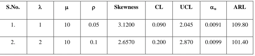
1.3 CONTROL CHART C3
In the queueing model (M / M / c) : ( / FCFS), the random variable N denote the number of customers in the system both waiting and in service. The steady state distribution of random variable N is given by expression (1). In order to obtain control limits using Shore’s method (2000), the first three moments of the random variable N given by expressions (6), (8) and (12) respectively, are needed.
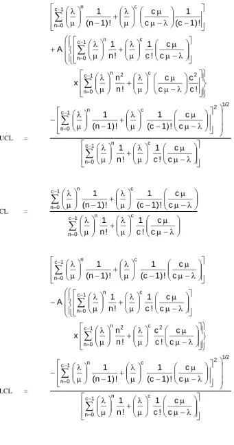
The expression (12) shows that skewness of the distribution of N depends on , , n and c. Taking into account the mean, standard deviation and skewness of the underlying geometric distribution of N the expression for the new control limits for the number of customers in (M / M / c) : ( / FCFS) system using Shore’s method (2000) are as follows :
www.ijsrp.org
UCL = E(N) +
3
V(N)
+ 1.324V(N)
Sk(N) 2
1
.
CL = E(N)
LCL = E(N)
3
V(N)
+ 1.324V(N)
Sk(N) +2
1
.
Control Limits for Control Chart C3 when Sk > 0.5
UCL = E(N) + 3.642
V(N)
+ 0.9146V(N)
Sk(N) 2
1
.
CL = E(N)
LCL = E(N) 3.642
V(N)
+ (1.40) (0.9146)V(N)
Sk(N) +2
1
.
Control Limits for Control Chart C3 for (M / M / c) : ( / FCFS) Model when Sk < 0.5
UCL =
c
c
!
1)
(c
1
!
1)
(n
1
c1 c
0 n
n
x
1 c
1 c
0 n
n
c
c
!
c
1
!
n
1
+ 3
c
c
!
c
1
!
n
1
c1 c
0 n
n
x
c
c
!
c
c
!
n
n
c 21 c
0 n
2 n
2 c
1 c
0 n
n
c
c
!
1)
(c
1
!
1)
(n
1
x
1 c
1 c
0 n
n
c
c
!
c
1
!
www.ijsrp.org + 1.324
c
c
!
c
1
!
n
1
c 1 c 0 n nx
c
c
!
c
c
!
n
n
c 21 c 0 n 2 n
2 c 1 c 0 n nc
c
!
1)
(c
1
!
1)
(n
1
x 1 1 c 1 c 0 n nc
c
!
c
1
!
n
1
x 2 c 1 c 0 n nc
c
!
c
1
!
n
1
x
c
c
!
c
c
!
n
n
c 31 c 0 n 3 n
3
c
c
!
c
1
!
n
1
c 1 c 0 n n x
c
c
!
1)
(c
1
!
1)
(n
1
c 1 c 0 n n x
c
c
!
c
c
!
n
n
c 21 c 0 n 2 n + 2
2
1
c
c
!
1)
(c
1
!
1)
(n
1
3 c 1 c 0 n nCL =
www.ijsrp.org x
1 c 1 c 0 n nc
c
!
c
1
!
n
1
LCL =
c
c
!
1)
(c
1
!
1)
(n
1
c 1 c 0 n n x
1 c 1 c 0 n nc
c
!
c
1
!
n
1
3
c
c
!
c
1
!
n
1
c 1 c 0 n nx
c
c
!
c
c
!
n
n
c 21 c 0 n 2 n
2 c 1 c 0 n nc
c
!
1)
(c
1
!
1)
(n
1
x
1 c 1 c 0 n nc
c
!
c
1
!
n
1
+ 1.324
c
c
!
c
1
!
n
1
c 1 c 0 n nx