A Weight Coded Evolutionary Algorithm for the Multidimensional Knapsack Problem

(1)

http://www.scirp.org/journal/apm ISSN Online: 2160-0384 ISSN Print: 2160-0368

A Weight-Coded Evolutionary Algorithm for the

Multidimensional Knapsack Problem

Quan Yuan, Zhixin Yang

Department of Mathematical Science, Ball State University, Muncie, IN, USA

Abstract

A revised weight-coded evolutionary algorithm (RWCEA) is proposed for solving multidimensional knapsack problems. This RWCEA uses a new decoding method and incorporates a heuristic method in initialization. Computational results show that the RWCEA performs better than a weight-coded evolutionary algorithm proposed by Raidl (1999) and to some existing benchmarks, it can yield better results than the ones reported in the OR-library.

Keywords

Weight-Coding, Evolutionary Algorithm, Multidimensional Knapsack Problem (MKP)

1. Introduction

The multidimensional knapsack problem (MKP) can be stated as:

( )

1

max ,

n j j j

f x p x

=

∑

_(1a)

1

s.t. , 1, , ,

n

ij j i j

r x b i m

=

≤ =

∑

 (1b)

{ }

0,1 , 1, , .

j

x ∈ j=  n (1c)

Each of the m constraints described in (1b) is called a knapsack constraint. A set of n items with profits p_j >0 and m resources with bi >0 are given. Each item j con-

sumes an amount r_ij ≥0 from each resource i. The 0-1 decision variables x_j indicate

which items are selected. A well-stated MKP also assumes that 1

n ij i j ij

r ≤b <

∑

₌ r and

0

j

p > for all i∈ =I

{

1,,m

}

, j∈ =J

{

1,,n

}

, since any violation of these condi-

tions will result in some constraints being eliminated or some xj’s being fixed.

How to cite this paper: Yuan, Q. and Yang, Z.X. (2016) A Weight-Coded Evolutionary Algorithm for the Multidimensional Knap-sack Problem. Advances in Pure Mathemat-ics, 6, 659-675.

http://dx.doi.org/10.4236/apm.2016.610055 Received: March 14, 2016

Accepted: September 16, 2016 Published: September 19, 2016

http://creativecommons.org/licenses/by/4.0/

(2)

660

The MKP degenerates to the knapsack problem when m=1 in Equation (1b). It is

well known that the knapsack problem is not a strong -hard problem and solvable

in pseudo-polynomial time. However, the situation is different to the general case of

1

m> . Garey and Johnson (1979) [1] proved that it is strongly -hard and exact

techniques are in practice only applicable to instances of small to moderate size. A real-world application example of MKP is selecting projects to fund. Assume there are n different projects and we need to select some projects and fund them for m years. Each project provides a profit and each of them has a budget determined for each year. Our objective is to maximize the total profit and not exceed yearly budgets. This prob-lem can be formulated as Equation (1). What is more, many practical probprob-lems such as the capital budgeting problem [2], allocating processors and databases in a distributed computer system [3], project selection and cargo loading [4], and cutting stock prob-lems [5] can be formulated as an MKP. The MKP is also a sub problem of many general integer programs.

Given the theoretical and practical importance of the MKP, a large number of papers have devoted to the problem. It is not the place here to recall all of these papers. We re-fer to the papers of Chu and Beasley (1998) [6], Fréville (2004) [7] and the monograph of Kellerer (2004) [8] for excellent overviews of theoretical analysis, exact methods, and heuristics of the MKP. Recently, some new algorithms for the MKP have been proposed such as some variants of the genetic algorithm [9], the ant colony algorithm [10], the scatter search method [11], and some new heuristics [12]-[15]. Some studies on analy-sis of the MKP [16], [17] and generalizations of the MKP [18]-[20] have also been put forward.

An Evolutionary algorithm (EA) is a generic population-based metaheuristic opti-mization algorithm. Candidate solutions to the optiopti-mization problem play the role of individuals (parents) in a population. Some mechanisms inspired by biological evolu-tion: selection, crossover and mutation are used. The fitness function determines the environment within which the solutions “survive”. Then new groups of the population (children) are generated after the repeated application of the above operators. EAs have found application in computational science, engineering, economics, chemistry, and many other fields (see [21]-[25]).

(3)

mentioned in [17] from empirical analysis.

The best success for solving the MKP, as far as we known, has been obtained with tabu-search algorithms embedding effective preprocessing [26], [27]. Recently, impres-sive results have also been obtained by an implicit enumeration [28], a convergent algo-rithm [29], and an exact method based on a multi-level search strategy [30]. Compared with EAs, the methods mentioned above can yield better results when excellent solu-tions are required. But they are more complicated to implement or their computation takes extremely long time. Since EAs are simple to implement and their computation time are easy to control, they are good alternatives if the quality requirement of solu-tions of the MKP is not very strict.

In this paper, we will consider a variant of EA to solve the MKP. This EA will use a special encoding technique which is called weight-coding (or weight-biasing). We will revise a weight-coded EA (WCEA) proposed by Raidl (1999) [31] and propose a revised weight-coded EA (RWCEA). The numerical experiments of some benchmarks will show that the RWCEA performs better than the WCEA. Moreover, this RWCEA can com-pete with DIH in some benchmarks.

2. An Introduction to the Weight-Coding and Its

Application to the MKP

When combinatorial optimization problems are solved by an EA, the coding of candidate solutions is a preliminary step. Direct coding such as the binary coding is an intui- tive method. The main drawback of this coding lies in that many infeasible solutions may be generated by EA’s operators. To avoid that, the basic idea of the weight-coding is to represent a candidate solution by a vector of real-valued weights w_j

(

j=1,,n

)

.

The phenotype that a weight vector represents is obtained by a two-step process. Step (a): (biasing) The original problem P is temporarily modified to P′_{by biasing}

problem parameters of P according to the weights wj;

Step (b): (decoding heuristic) A problem-specific decoding heuristic is used to generate a solution to P′_{. This solution is interpreted and evaluated for the original (unbia-}

sed) problem P.

The weight-coding is an interesting approach because it can eliminate the necessity of an explicit repair algorithm, a penalization of infeasible solutions, or special crossover and mutation operators. It has already been successfully used for a variety of problems such as an optimum communications spanning tree problem [32], problem [33], the traveling salesman problem [34], and the multiple container packing problem [35].

To the best of the authors’ knowledge, the work of Raidl (1999) [31] is the first to use weight-coded EA (WCEA) to deal with the MKP. In that paper, some variants of WCEAs were proposed and compared. And Raidl finally suggested one of them and compared the WCEA with other EAs in [17]. In this WCEA, wj

(

j=1,,n

)

is set to be the

weight vector representing a candidate solution. Weight wj is associated with item j

(4)

662

(

)

( )0,1

1 , 1, ,

j j j j

p′ = p w = p +γ  j=  n (2)

where 

( )

0,1 denotes a normally distributed random number with mean 0 and stan-

dard deviation 1, and γ >0 is a strategy parameter that controls the average intensity

of biasing. Raidl (1999) [31] suggested that γ =0.05. Since the resource consumption

values rij and resource limits bi are not modified, all feasible solutions of the biased

MKP are feasible to (1).

Corresponding to Step (b), the decoding heuristic which Raidl (1999) [31] suggested is making use of the surrogate relaxation (see [36], [37]). The m resource constraints (1b) are aggregated into a single constraint using surrogate multipliers ai, i=1,,m:

1 1 1

n m m i ij j i i j i i

a r x a b

= = =

  _≤

 

 

∑ ∑

∑

(3)

where ai are obtained by solving the linear programming (LP) of the relaxed MKP, in

which the variables xj may get real values from

[ ]

0,1 . The values of the dual varia-

bles are then used as surrogate multipliers, i.e. ai is set to the shadow price of the i-th

constraint in the LP-relaxed MKP. Pseudo-utility ratios are defined as:

1

.

j j m

i ij i

p u

a r

=

′ =

∑

(4)

A higher pseudo-utility ratio heuristically indicates that an item is more efficient. After the items are sorted by decreasing order of uj, the first-fit strategy used as

decoder in the permutation representation is applied. All items are checked one by one and each item’s variable xj is set to 1 if no resource constraint is violated, otherwise,

j

x is set to 0. The computational effort of the decoder is O n

(

⋅logn

)

for sorting the

j

u plus O n m

(

⋅

)

for the first-fit strategy, yielding O n

(

⋅

(

m+logn

)

in total.

Raidl’s WCEA can be described as follows (we will explain the details of Steps 6, 7, and 8 afterward):

Algorithm of Raidl’s WCEA Step 1: set t: 0= ;

Step 2: initialize pop t

( ) {

= S1,,SN

}

, Si=

(

w1,,wn

)

where wj is a random va-

lue following log-normally distribution as (2); Step 3: evaluate pop t

( )

:

{

f S

( )

1 ,,f S

( )

N

}

;

for each Si

3-1: bias original MKP;

3-2: use decoding heuristic as in [31] (described above) to get phenotype

( ) { }

S_i ∈ 0,1n

P ;

3-3: substitute P

( )

Si into (1a) to obtain f S

( )

i ;

Step 4: find *

( )

S ∈pop t s.t.

( )

*

( )

f S ≥ f S , ∀ ∈S pop t

( )

; t<t_max do

Step 5: select

{

p p1, 2

}

from pop t

( )

;

Step 6: crossover p1 and p2 to generate a child C;

Step 7: mutate C;

(5)

Step 9: if P

( )

C ≡ any P

( )

Si then (that means C is a duplicate of a member of the

population)

Step 10: discard C and goto Step 6; end if

Step 11: find S′∈pop t

( )

s.t. f S

( )

′ ≤ f S

( )

∀ ∈S pop t

( )

and replace S′ ←C;

(steady-state replacement, i.e., the worst individual of population is replaced). Step 12: if _{f C}

( )

_> _{f S}

( )

* then

Step 13: *

S ←C; (update best solution S* found)

end if

Step 14: t← +t 1;

end while

Step 15: return *

S , f S

( )

* .

In Step 6, a binary tournament selection is used. That is, two pools of individuals, which consist of 2 individuals drawn from the population randomly, are formed re- spectively at first. Then two individuals with the best fitness, each taken from one of the two tournament pools, are chosen to be parents.

In Step 7, Raidl (1999) [31] suggested a uniform crossover instead of one- or two- point crossover. In the uniform crossover two parents have one child. Each

(

1, ,

)

j

w j=  n in the child is chosen randomly by copying the corresponding weight

from one or the other parent.

Once a child has been generated through the crossover, a mutation step in Step 8 is performed. Each wj of the child is reset to a new random value observing log-normal

distribution with a small probability (3/n per weight as in [31] or one random position in [17]).

In numerical experiments, the N in Step 2 is taken as 100 and tmax in Step 5 is taken

106_{. Raidl and Gottlieb (2005)}_[17]_{compared this WCEA with other five EAs for the}

MKP. From empirical analysis, this WCEA outperformed all of them except DIH (The meaning of DIH is given in Section 1) on average.

3. Our Revised WCEA for the MKP

3.1. Motivation

The core of Raidl’s WCEA is the surrogate relaxation based heuristic in decoding. In our points of view, this heuristic has two drawbacks. First, the dual variables of an LP- relaxed MKP used in heuristic decoding step are just good approximations of optimal surrogate multipliers and it may mislead the search [26]. LP-relaxed MKP used in heuristic decoding step are just approximations of optimal surrogate multipliers. And deriving optimal surrogate multipliers is a difficult task in practice [38]. Secondly, the heuristic decoding might mislead the search if the optimal solution is not very similar to the solution generated by applying the greedy heuristic [39].

In order to avoid using surrogate multipliers, we set w_j

(

j=1,,n

)

to let every w_j

observe uniform distribution on 0,pmax pj, where pmax =max

{

pj: j=1,,n

}

. The

(6)

664

, 1, , .

j j j

p′ =p w j=  n (5)

as mentioned in Section II, all feasible solutions of this biased MKP are feasible to (1). In decoding heuristic, we also use first-fit strategy, i.e., the items are sorted by decreasing order of p′j (not by pseudo-utility ratio in (4)) and traversed. Each item’s

variable xj is set to 1 if no resource constraint is violated. The computational effort of

the decoder is also O n

(

⋅

(

m+logn

)

in total.

This form of wj is similar to the idea of Random-key Representation [40]. Surro-

gate multipliers can be avoided but the efficiency of the EA will be reduced [17]. To overcome this disadvantage, our thought is to obtain a “good” initial population. In the following we first introduce an idea proposed by Vasquez and Hao [26] and then propose our method.

It is well known that only relaxing the integrality constraints in an MKP may not be sufficient because its optimal solution may be far away from the optimal binary solution. However, Vasquez and Hao in [26] observed when the integrality constraints was replaced by a hyperplane constraint 1

n j j=x = ∈k

∑

, the corresponding linear programming solution may often be close to the optimal binary solution. For example in

[26], in (1) we let n=5, m=1, p=

{

12,12,9,8,8

}

, r=

{

11,12,10,10,10

}

, b=30. The

relax linear programming problem leads to the fractional optimal solution

{

1,1, 0.7, 0, 0

}

LP

x = while the optimal binary solution is x=

{

0, 0,1,1,1

}

. If we replace

the integrality constraints by 1 3

n j j= x =

∑

, this linear programming problem leads to the optimal binary solution.

In the above example, if we take w=

{

0, 0,1,1,1

}

and substitute it to (5), the optimal

binary solution can be obtained by first-fit heuristic mentioned above. Moreover, if we do not restrict k as an integer, we may also obtain some corresponding linear programming solutions from which some good binary solutions may be obtained by first-fit heuristic. We use these linear programming solutions as a “good” initial population. So the disadvantage of Random-key Representation may be overcome. The experimental results presented later have confirmed this hypothesis. Naturally, the hypothesis does not exclude the possibility that there exists a certain MKP whose optimal binary solution cannot be obtained from linear programming solutions.

Inspired by this idea, initialization is guided by the LP relaxation with a hyperplane constraint. To begin with, we use some simple heuristic (such as a greedy algorithm) to obtain a 0 - 1 lower bound z. Next, the two following problems:

max 1 max , n j j k x = =

∑

1

s.t. , 1, , ,

n

ij j i j

r x b i m

= ≤ =

∑

 1 1 n j j j

p x z

=

≥ +

∑

[ ]

0,1 , 1, ,

j

x ∈ j=  n

(7)

min 1 min , n j j k x = =

∑

1

s.t. , 1, , ,

n

ij j i j

r x b i m

= ≤ =

∑



1

1 =

+

≥

∑

p

_j

x

_j

z

n

j

[ ]

0,1 , 1, ,

j

x ∈ j=  n

are solved to obtain kmax and kmin.

Then, N linear programming problems

1

max ,

s.t. , 1, , ,

[0,1], 1, ,

n j j j n

ij j i j n j j j p x

r x b i m

x k

x j n

= = = ≤ = ′ = ∈ =

∑

  (6)

are solved where k′ is a real number generated randomly from

[

kmin,kmax

]

in each

computation. So the N linear programming solutions are generated as the initial population.

3.2. Implementation

The scheme of the RWCEA is as follows: Algorithm of the RWCEA

Step 1: set t: 0= ;

Step 2: initialize pop t

( ) {

= S1,,SN

}

by solving N linear programming problems

of (6), Si=

(

w1,,wn

)

.

3-1: bias original MKP;

3-2: use decoding heuristic as in [31] (described in Section 2) to get phenotype

( ) { }

Si ∈ 0,1n

P ;

3-3: substitute P

( )

Si into (1a) to obtain f S

( )

i ;

Step 3: find *

( )

S ∈pop t s.t.

( )

*

( )

f S ≥ f S , ∀ ∈S pop t

( )

; t<tmax do

Step 4: select

{

p p1, 2

}

from pop t

( )

;

Step 5: crossover p1 and p2 to generate a child C;

Step 6: mutate C: one random wj of the child is reset to a new random value ob-

serving uniform distribution on 0,pmax pj;

Step 7: evaluate C as Step 3, get P

( )

C and f C

( )

;

Step 8: if P

( )

C ≡ any P

( )

Si then (that means C is a duplicate of a member of

the population);

(8)

666

Step 10: find S′∈pop t

( )

s.t. f S

( )

′ ≤ f S

( )

∀ ∈S pop t

( )

and replace S′ ←C;

(steady-state replacement, i.e., the worst individual of population is replaced). Step 11: if

( )

*

f C > f S then

Step 12: *

S ←C; (update best solution S* found)

end if

Step 13: t← +t 1;

end while

Step 14: return *

S , _{f S}

( )

* .

The scheme of the RWCEA is similar to Raidl’s WCEA. And we take the same values of N and tmax as the WCEA. The differences between the two algorithms lie in the

following aspects:

1) The initial population in Raidl’s WCEA is generated randomly, while in the RWCEA, N linear programming problems should be solved;

2) Each wj in Raidl’s WCEA observes log-normal distribution, while in RWCEA it

observes a uniform distribution on 0,pmax pj, where pmax =max

{

pj: j=1,,n

}

;

3) Raidl’s WCEA sorts items by pseudo-utility ratios in heuristic decoding step while the RWCEA sorts items by biased profits directly;

4) In the mutation step, one random wj of the child is reset to a new random value

observing uniform distribution on 0,pmax pj instead of log-normal distribution in

the RWCEA.

In summary, we revised Raidl’s WCEA by avoiding using surrogate multipliers and using “good” initial population. We think this RWCEA can yield better result than WCEA in some instances of MKP. The performance of RWCEA is shown in the next section.

4. Experimental Comparison

As in [17], two test suites of MKP’s benchmark instances for experimental comparison are used in this paper. The first one, referred to as CB-suite in this paper, is introduced by Chu and Beasley (1998) [6] and is available in the OR-Library1_{. This test suite}

contains 270 instances for each 10 ones are combination of m∈

{

5,10, 30

}

constraints,

{

100, 250, 500

}

n∈ items, and tightness ratio α∈

{

0.25, 0.5, 0.75

}

. Each problem has

been generated randomly such that 1

n i j ij

b = ⋅α

∑

₌r for all i=1,,m. Chu and Beasley

used their GA (i.e., DIH) to solve these instances and reported their results in the OR- library. The second MKP’s benchmark suite2_{used in}_[17]_{was first referenced by}_[26]

and originally provided by Glover and Kochenberger. These instances, called GK01 to GK11, range from 100 to 2500 items and from 15 to 100 constraints. We call this suite GK-suite in this paper.

Although some commercial integral linear programming (ILP) solvers, such as CPLEX, can solve ILP problems with thousands of integer variables or even more, it seems that the MKP remains rather difficult to handle when an optimal solution is wanted. To CB- suit, the results in [6] showed that major instances of this suit cannot be solved in a

1_{http://people.brunel.ac.uk/~mastjjb/jeb/info.html}_.

(9)

reasonable amount of CPU time and memory by CPLEX. To GK-suit, which includes still more difficult instances with n up to 2500, Fréville (2004) in [7] mentioned that CPLEX cannot tackle these instances. Therefore, it appears that the MKP continues to be a challenging problem for commercial ILP solvers.

The best known solutions to these benchmarks, as far as we known, were obtained by Vasquez and Hao (2001) [26] and was improved by Vasquez and Vimont (2005) [27]. Their method is based on tabu search and time-consuming compared with EA.

Raidl and Gottlieb (2005) [17] tested six different variants of EAs, which are called Permutation Representation (PE), Ordinal Representation (OR), Random-Key Represen- tation (RK), Weight-Biased Representation (WB), i.e. Raidl’s WCEA, and Direct Repre- sentation (DI and DIH). We compare the RWCEA with these EAs except DIH first. We use all GK-suite and draw out nine instances (called CB1 to CB9) from CB-suite, which are the first instances with α =0.5 for each combination of m and n.

For a solution x, the gap is defined as:

( )

LP

f x f x

gap

f x

− =

where LP

x is the optimum of the LP-relaxed problem to measure the quality of x.

We implement the RWCEA on a personal computer (Inter CoreTM_{Duo T5800, 2}

GHz, 1.99 GB main memory, Windows XP) using DEV-C++. The initial population is generated by MATLAB. The population size is 100, and each run was terminated after 106_{created solution candidates; rejected duplicates were not counted.}

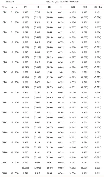
Table 1 shows the average gaps of the final solutions and their standard deviations obtained from independent 30 runs per problem instance obtained by the RWCEA and other six variants. The results of other six variants come from [17]. In the last column, bold fonts mean that the results of RWCEA is the best (or equally best) in the seven EAs. Italics in the last column mean that the results of RWCEA is better or equal than PE, OR, RK, DI, and WCEA but slightly worse than DIH. From this table we can draw the conclusion that the RWCEA is an improvement of WCEA. Especially in GK02 to GK11, the RWCEA performed much better than Raidl’s method.

Table 1 also shows that the RWCEA performed averagely slightly worse than DIH. But we will point out that can yield better results than DIH in some instances. Since the best results can be obtained by CPLEX in CB-suite when

{ } {

m n, = 5,100

}

,

{

10,100

}

,

and

{

5, 250

}

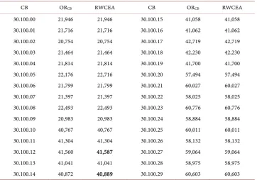
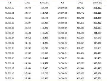
, we tested the other 180 instances in CB-suite. Each instance was com-

puted 30 times and the best results were compared with the results reported in OR- library. The data of the numbers that the RWCEA yielded better, equal or worse results than the results reported in OR-library is shown in Table 2. Tables 3-8 show the comparison of each instance. These tables show that the results of more than 50% instances can be improved by the RWCEA.

5. Conclusion

(10)

[image:10.595.194.549.106.712.2]

668

Table 1. Average gaps of best solutions and their standard deviations of the RWCEA and other EAs.

Instance Gap [%] (and standard deviation)

Name m n PE OR RK DI WB DIH RWCEA

CB1 5 100 0.425 0.745 0.425 0.425 0.425 0.425 0.425 (0.000) (0.210) (0.000) (0.000) (0.000) (0.000) (0.000) CB2 5 250 0.120 1.321 0.115 0.150 0.106 0.106 0.112

(0.012) (0.346) (0.009) (0.019) (0.007) (0.006) (0.007) CB3 5 500 0.081 2.382 0.065 0.121 0.042 0.038 0.036

(0.016) (0.657) (0.010) (0.020) (0.008) (0.003) (0.004) CB4 10 100 0.762 1.013 0.762 0.770 0.761 0.762 0.762

(0.001) (0.163) (0.003) (0.013) (0.000) (0.003) (0.003) CB5 10 250 0.295 1.498 0.277 0.324 0.249 0.261 0.271

(0.033) (0.225) (0.021) (0.043) (0.017) (0.008) (0.014) CB6 10 500 0.225 2.815 0.200 0.263 0.131 0.112 0.108

(0.040) (0.462) (0.029) (0.040) (0.014) (0.007) (0.002) CB7 30 100 1.372 1.800 1.338 1.401 1.319 1.336 1.276

(0.134) (0.182) (0.123) (0.073) (0.093) (0.091) (0.077) CB8 30 250 0.608 2.076 0.611 0.599 0.535 0.519 0.525

(0.048) (0.346) (0.072) (0.059) (0.031) (0.013) (0.002) CB9 30 500 0.429 3.267 0.376 0.463 0.306 0.288 0.296

(0.058) (0.442) (0.037) (0.056) (0.024) (0.012) (0.012) GK01 15 100 0.377 0.683 0.384 0.336 0.308 0.270 0.325

(0.068) (0.098) (0.080) (0.074) (0.077) (0.028) (0.077) GK02 25 100 0.503 0.959 0.521 0.564 0.481 0.460 0.458

(0.062) (0.144) (0.068) (0.067) (0.045) (0.007) (0.000) GK03 25 150 0.517 1.002 0.531 0.517 0.452 0.366 0.374

(0.060) (0.140) (0.077) (0.066) (0.042) (0.007) (0.034) GK04 50 150 0.712 1.164 0.748 0.706 0.669 0.528 0.527

(0.090) (0.143) (0.098) (0.079) (0.081) (0.021) (0.027) GK05 25 200 0.462 1.124 0.552 0.493 0.397 0.294 0.289

(0.072) (0.153) (0.118) (0.087) (0.046) (0.004) (0.012) GK06 50 200 0.703 1.236 0.751 0.714 0.611 0.429 0.417

(0.070) (0.141) (0.108) (0.077) (0.060) (0.018) (0.015) GK07 25 500 0.523 1.468 0.651 0.496 0.382 0.093 0.111

(0.088) (0.092) (0.087) (0.089) (0.082) (0.004) (0.005)

(11)

Continued

(0.086) (0.109) (0.125) (0.085) (0.066) (0.006) (0.013) GK09 25 1500 0.890 2.312 1.064 0.695 0.558 0.029 0.030

(0.075) (0.113) (0.133) (0.070) (0.042) (0.001) (0.001) GK10 50 1500 1.101 1.883 1.177 0.950 0.727 0.052 0.053

(0.065) (0.076) (0.082) (0.090) (0.070) (0.003) (0.002) GK11 100 2500 1.237 1.677 1.246 1.161 0.867 0.052 0.056

(0.060) (0.056) (0.067) (0.063) (0.061) (0.002) (0.002) average 0.605 1.597 0.631 0.595 0.493 0.329 0.331

[image:11.595.195.554.284.409.2]

(0.057) (0.215) (0.068) (0.057) (0.043) (0.012) (0.015)

Table 2. The data of the numbers that the RWCEA yielded better, equal and worse results than the results reported in OR-library.

m n Number of the instance Better Equal Worse

30 100 30 2 28 0

10 250 30 12 16 2

30 250 30 15 10 5

5 500 30 19 9 2

10 500 30 23 4 3

30 500 30 21 4 5

Total 180 92 71 17

Table 3. The results of CB-suite reported in OR-library (ORCB) and the ones obtained by the

RWCEA (m=30, n=100).

CB ORCB RWCEA CB ORCB RWCEA

30.100.00 21,946 21,946 30.100.15 41,058 41,058

30.100.01 21,716 21,716 30.100.16 41,062 41,062

30.100.02 20,754 20,754 30.100.17 42,719 42,719

30.100.03 21,464 21,464 30.100.18 42,230 42,230

30.100.04 21,814 21,814 30.100.19 41,700 41,700

30.100.05 22,176 22,716 30.100.20 57,494 57,494

30.100.06 21,799 21,799 30.100.21 60,027 60,027

30.100.07 21,397 21,397 30.100.22 58,025 58,025

30.100.08 22,493 22,493 30.100.23 60,776 60,776

30.100.09 20,983 20,983 30.100.24 58,884 58,884

30.100.10 40,767 40,767 30.100.25 60,011 60,011

30.100.11 41,304 41,304 30.100.26 58,132 58,132

30.100.12 41,560 41,587 30.100.27 59,064 59,064

30.100.13 41,041 41,041 30.100.28 58,975 58,975

[image:11.595.193.556.453.707.2]

(12)

670

RWCEA (m=10, n=250).

10.250.00 59,187 59,187 10.250.15 110,841 110,841

10.250.01 58,662 58,708 10.250.16 106,075 106,075

10.250.02 58,094 58,094 10.250.17 106,686 106,686

10.250.03 61,000 61,000 10.250.18 109,825 109,825 10.250.04 58,092 58,092 10.250.19 106,723 106,723 10.250.05 58,803 58,803 10.250.20 151,790 151,801 10.250.06 58,607 58,704 10.250.21 147,822 148,772 10.250.07 58,917 58,930 10.250.22 151,900 151,900 10.250.08 59,384 59,382 10.250.23 151,275 151,281 10.250.09 59,193 59,208 10.250.24 151,948 151,966 10.250.10 110,863 110,913 10.250.25 152,109 151,209 10.250.11 108,659 108,702 10.250.26 153,131 153,131 10.250.12 108,932 108,932 10.250.27 153,520 153,578 10.250.13 110,037 110,034 10.250.28 149,155 149,160

[image:12.595.194.556.102.383.2]

10.250.14 108,423 108,485 10.250.29 149,704 149,704

RWCEA (m=30, n=250).

30.250.00 56,693 56,747 30.250.15 107,246 107,183

30.250.01 58,318 58,520 30.250.16 106,308 106,261

30.250.02 56,553 56,553 30.250.17 103,993 103,993

[image:12.595.193.556.426.708.2]

(13)

[image:13.595.193.555.100.379.2]

RWCEA (m=5, n=500).

5.500.00 120,130 120,145 5.500.15 220,514 220,520

5.500.01 117,837 117,864 5.500.16 219,987 219,989

5.500.02 121,109 121,118 5.500.17 218,194 218,215

5.500.03 120,798 120,798 5.500.18 216,976 216,976 5.500.04 122,319 122,319 5.500.19 219,693 219,719 5.500.05 122,007 122,009 5.500.20 295,828 295,828 5.500.06 119,113 119,127 5.500.21 308,077 308,083 5.500.07 120,568 120,568 5.500.22 299,796 299,796 5.500.08 121,575 121,575 5.500.23 306,476 306,480 5.500.09 120,699 120,717 5.500.24 300,342 300,342 5.500.10 218,422 218,428 5.500.25 302,560 302,559 5.500.11 221,191 221,188 5.500.26 301,322 301,329 5.500.12 217,534 217,542 5.500.27 296,437 296,457 5.500.13 223,558 223,560 5.500.28 306,430 306,454 5.500.14 218,962 218,966 5.500.29 299,904 299,904

RWCEA (m=10, n=500).

10.500.00 117,726 117,779 10.500.15 215,013 215,041

10.500.01 119,139 119,181 10.500.16 217,896 217,911

10.500.02 119,159 119,194 10.500.17 219,949 219,984 10.500.03 118,802 118,784 10.500.18 214,332 214,346 10.500.04 116,434 116,471 10.500.19 220,833 220,865 10.500.05 119,454 119,461 10.500.20 304,344 304,344 10.500.06 119,749 119,777 10.500.21 302,332 302,333 10.500.07 118,288 118,277 10.500.22 302,354 302,408 10.500.08 117,779 117,750 10.500.23 300,743 300,747 10.500.09 119,125 119,175 10.500.24 304,344 304,350 10.500.10 217,318 217,318 10.500.25 301,730 301,757 10.500.11 219,022 219,033 10.500.26 304,949 304,949 10.500.12 217,772 217,772 10.500.27 296,437 296,457 10.500.13 216,802 216,819 10.500.28 301,313 301,353

[image:13.595.192.557.426.707.2]

(14)

[image:14.595.193.555.102.375.2]

672

RWCEA (m=30, n=500).

30.500.00 115,868 115,864 30.500.15 215,762 215,832 30.500.01 114,667 114,701 30.500.16 215,772 215,839 30.500.02 116,661 116,661 30.500.17 216,336 216,419 30.500.03 115,237 115,228 30.500.18 217,290 217,302 30.500.04 116,353 116,370 30.500.19 214,624 214,634 30.500.05 115,604 115,639 30.500.20 301,627 301,643 30.500.06 113,952 113,983 30.500.21 299,985 299,958 30.500.07 114,199 114,230 30.500.22 304,995 305,062 30.500.08 115,247 115,247 30.500.23 301,935 301,935 30.500.09 116,947 116,947 30.500.24 304,404 304,411 30.500.10 217,995 218,042 30.500.25 296,894 296,955 30.500.11 214,534 214,557 30.500.26 303,233 303,262 30.500.12 215,854 215,885 30.500.27 306,944 306,985 30.500.13 217,836 217,773 30.500.28 303,057 303,120 30.500.14 215,566 215,553 30.500.29 300,460 300,531

RWCEA has been different from Raidl’s WCEA in the ways that surrogate multipliers are not used and a heuristic method is incorporated in initialization. Experimental comparison has shown that the RWCEA can yield better results than Raidl’s WCEA in [31]

and better results than the ones reported in the OR-library to some existing bench-marks. So we think this RWCEA is a good opinion in solving MKPs. A more detailed investigation of the working mechanism of the RWCEA and the application of RWCEA to other variants of knapsack problems (such as multiple choice multidimensional knapsack problems) will be the subjects of further work.

References

[1] Garey, M.R. and Johnson, D.S. (1979) Computers and Intractability: A Guide to the Theory of NP-Completeness. W. H. Freeman & Co., New York.

[2] Markowitz, H.M. and Manne, A.S. (1957) On the Solution of Discrete Programming Prob-lems. Econometrica, 25, 84-110. http://dx.doi.org/10.2307/1907744

[3] Gavish, B. and Pirkul, H. (1982) Allocation of Databases and Processors in a Distributed Computing System. In: Akoka, J., Ed., Management of Distributed Data Processing, North-Holland, 31, 215-231.

[4] Shih, W. (1979) A Branch and Bound Method for the Multiconstraint Zero-One Knapsack Problem. Journal of the Operational Research Society, 30, 369-378.

http://dx.doi.org/10.1057/jors.1979.78

(15)

[6] Chu, P.C. and Beasley, J.E. (1998) A Genetic Algorithm for the Multidimensional Knapsack Problem. Journal of Heuristics, 4, 63-86. http://dx.doi.org/10.1023/A:1009642405419

[7] Fréville, A. (2004) The Multidimensional 0−1 Knapsack Problem: An Overview. European Journal of Operational Research, 155, 1-21.

http://dx.doi.org/10.1016/S0377-2217(03)00274-1

[8] Kellerer, H., Pferschy, U. and Pisinger, D. (2004) Knapsack Problems. Springer, Berlin.

http://dx.doi.org/10.1007/978-3-540-24777-7

[9] Li, H., Jiao, Y., Zhang, L. and Gu, Z. (2006) Genetic Algorithm Based on the Orthogonal Design for Multidimensional Knapsack Problems. Advances in Natural Computation. Springer Berlin/Heidelberg, 696-705.

[10] Kong, M., Tian, P. and Kao, Y. (2008) A New Ant Colony Optimization Algorithm for the Multidimensional Knapsack Problem. Computers & Operations Research, 35, 2672-2683.

http://dx.doi.org/10.1016/j.cor.2006.12.029

[11] Hanafi, S. and Wilbaut, C. (2008) Scatter Search for the 0−1 Multidimensional Knapsack Problem. Journal of Mathematical Modelling and Algorithms, 7, 143-159.

http://dx.doi.org/10.1007/s10852-008-9078-9

[12] Boyer, V., Elkihel, M. and El Baz, D. (2009) Heuristics for the 0−1 Multidimensional Knap-sack Problem. European Journal of Operational Research, 199, 658-664.

http://dx.doi.org/10.1016/j.ejor.2007.06.068

[13] Fleszar, K. and Hindi, K.S. (2009) Fast, Effective Heuristics for the 0−1 Multi-Dimensional Knapsack Problem. Computers & Operations Research, 36, 1602-1607.

[14] Puchinger, J., Raidl, G.R. and Gruber, M. (2005) Cooperating Memetic and Branch-and- Cut Algorithms for Solving the Multidimensional Knapsack Problem. Proceeding of the 6th Metaheuristics International Conference, Vienna, 22-26 August 2005, 775-780.

[15] Zou, D., Gao, L., Li, S., et al. (2011) Solving 0−1 Knapsack Problem by a Novel Global Harmony Search Algorithm. Applied Soft Computing, 11, 1556-1564.

http://dx.doi.org/10.1016/j.asoc.2010.07.019

[16] Fréville, A. and Hanafi, S. (2005) The Multidimensional 0−1 Knapsack Problem—Bounds and Computational Aspects. Annals of Operations Research, 139, 195-227.

http://dx.doi.org/10.1007/s10479-005-3448-8

[17] Raidl, G.R. and Gottlieb, J. (2005) Empirical Analysis of Locality, Heritability and Heuristic bias in Evolutionary Algorithms: A Case Study for the Multidimensional Knapsack Prob-lem. Evolutionary Computation, 13, 441-475.

http://dx.doi.org/10.1162/106365605774666886

[18] Changdar, C., Mahapatra, G.S. and Pal, R.K. (2013) An Ant Colony Optimization Ap-proach for Binary Knapsack Problem under Fuzziness. Applied Mathematics and Compu-tation, 223, 243-253. http://dx.doi.org/10.1016/j.amc.2013.07.077

[19] Hifi, M., M’Halla, H. and Sadfi, S. (2005) An Exact Algorithm for the Knapsack Sharing Problem. Computers & Operations Research, 32, 1311-1324.

[20] Mavrotas, G., Figueira, J.R. and Florios, K. (2009) Solving the Bi-Objective Multi-Dimen- sional Knapsack Problem Exploiting the Concept of Core. Applied Mathematics and Com-putation, 7, 2502-2514. http://dx.doi.org/10.1016/j.amc.2009.08.045

[21] Yuan, Q., Qian, F. and Du, W. (2010) A Hybrid Genetic Algorithm with the Baldwin Effect.

Information Sciences, 180, 640-652. http://dx.doi.org/10.1016/j.ins.2009.11.015

(16)

674

Optimization Problems with Box Constraints. Applied Mathematics and Computation, 197, 924-929. http://dx.doi.org/10.1016/j.amc.2007.08.081

[23] Yuan, Q. and Qian, F. (2010) A Hybrid Genetic Algorithm for Twice Continuously Diffe-rentiable NLP Problems. Computers & Chemical Engineering, 34, 36-41.

http://dx.doi.org/10.1016/j.compchemeng.2009.09.006

[24] Yuan, Q., He, Z. and Leng, H. (2008) An Evolution Strategy Method for Computing Eigen-value Bounds of Interval Matrices. Applied Mathematics and Computation, 196, 257-265.

http://dx.doi.org/10.1016/j.amc.2007.05.051

[25] Yuan, Q. and Yang, Z. (2013) On the Performance of a Hybrid Genetic Algorithm in Dy-namic Environments. Applied Mathematics and Computation, 219, 11408-11413.

http://dx.doi.org/10.1016/j.amc.2013.06.006

[26] Vasquez, M. and Hao, J.-K. (2001) A Hybrid Approach for the 0−1 Multidimensional Knapsack Problem. Proceeding of the 17th International Joint Conference on Artificial In-telligence, Seattle, 4-10 August 2001, 328-333.

[27] Vasquez, M. and Vimont, Y. (2005) Improved Results on the 0−1 Multidimensional Knap-sack Problem. European Journal of Operational Research, 165, 70-81.

http://dx.doi.org/10.1016/j.ejor.2004.01.024

[28] Vimont, Y., Boussier, S. and Vasquez, M. (2008) Reduced Costs Propagation in an Efficient Implicit Enumeration for the 0−1 Multidimensional Knapsack Problem. Journal of Com-binatorial Optimization, 15, 165-178. http://dx.doi.org/10.1007/s10878-007-9074-4

[29] Hanafi, S. and Wilbaut, C. (2011) Improved Convergent Heuristic for the 0−1 Multidimen-sional Knapsack Problem. Annals of Operations Research, 183, 125-142.

http://dx.doi.org/10.1007/s10479-009-0546-z

[30] Boussier, S., Vasquez, M., Vimont, Y., Hanafi, S. and Michelon, P. (2010) A Multi-Level Search Strategy for the 0−1 Multidimensional Knapsack Problem. Discrete Applied Ma-thematics, 158, 97-109. http://dx.doi.org/10.1016/j.dam.2009.08.007

[31] Raidl, G.R. (1999) Weight-Codings in a Genetic Algorithm for the Multiconstraint Knap-sack Problem. Proceedings of the 1999 Congress on Evolutionary Computation, Washing-ton DC, 6-9 July 1999, 596-603. http://dx.doi.org/10.1109/CEC.1999.781987

[32] Palmer, C.C. and Kershenbaum, A. (1994) Representing Trees in Genetic Algorithms. Pro-ceeding of the 1st IEEE International Conference of Evolutionary Computation, Orlando, 27-29 June 1994, 379-384. http://dx.doi.org/10.1109/icec.1994.349921

[33] Capp, K. and Julstrom, B. (1998) A Weight-Coded Genetic Algorithm for the Minimum Weight Triangulation Problem. Proceeding of 1998 ACM Symposium on Applied Compu-ting,Atlanta, 27February-1 March 1998, 327-331. http://dx.doi.org/10.1145/330560.330833

[34] Julstrom, B. (1998) Comparing Decoding Algorithms in a Weight-Coded GA for TSP. Pro-ceeding of 1998 ACM Symposium on Applied Computing,Atlanta, 27February-1 March 1998, 313-317. http://dx.doi.org/10.1145/330560.330830

[35] Raidl, G.R. (1999) A Weight-Coded Genetic Algorithm for the Multiple Container Packing Problem. Proceeding of the 14th ACM Symposium on Applied Computing, San Antonio, 28 February-2 March 1999, 291-296. http://dx.doi.org/10.1145/298151.298354

[36] Glover, F. (1975) Surrogate Constraint Duality in Mathematical Programming. Operations Reserach, 23, 434-451. http://dx.doi.org/10.1287/opre.23.3.434

[37] Hanafi, S. and Féville, A. (1998) An Efficient Tabu Search Approach for the 0−1 Multidi-mensional Kanpsack Problem. European Journal of Operational Research, 106, 659-675.

http://dx.doi.org/10.1016/S0377-2217(97)00296-8

(17)

Knapsack Problems to Optimality. Mathematical Programming, 31, 78-105.

http://dx.doi.org/10.1007/BF02591863

[39] Rothlauf, F. and Goldberg, D.E. (2003) Redundant Representation in Evolutionary Com-putation. Evolutionary Computation, 11, 381-415.

http://dx.doi.org/10.1162/106365603322519288

[40] Hinterding, R. (1999) Representation, Constraint Satisfaction and the Knapsack Problem.

Proceedings of the 1999 Congress on Evolutionary Computation, Washington DC, 6-9 July 1999, 1286-1292. http://dx.doi.org/10.1109/CEC.1999.782591

Submit or recommend next manuscript to SCIRP and we will provide best service for you:

Accepting pre-submission inquiries through Email, Facebook, LinkedIn, Twitter, etc. A wide selection of journals (inclusive of 9 subjects, more than 200 journals)

Providing 24-hour high-quality service User-friendly online submission system Fair and swift peer-review system

Efficient typesetting and proofreading procedure

Display of the result of downloads and visits, as well as the number of cited articles Maximum dissemination of your research work

Submit your manuscript at: http://papersubmission.scirp.org/