http://www.scirp.org/journal/wjnst ISSN Online: 2161-6809
ISSN Print: 2161-6795
Method to Measure Indoor Radon Concentration
in an Open Volume with Geiger-Mueller Counters:
Analysis from First Principles
M. P. Silverman
Department of Physics, Trinity College, Hartford, CT, USA
Abstract
A simple method employing a pair of pancake-style Geiger-Mueller (GM) counters for quantitative measurement of radon activity concentration (activity per unit vo-lume) is described and demonstrated. The use of two GM counters, together with the basic theory derived in this paper, permit the detection of alpha particles from decay of 222
Rn and progeny (218Po, 214Po) and the conversion of the alpha count rate
into a radon concentration. A unique feature of this method, in comparison with standard methodologies to measure radon concentration, is the absence of a fixed control volume. Advantages afforded by the reported GM method include: 1) it pro-vides a direct in-situ value of radon level, thereby eliminating the need to send sam-ples to an external testing laboratory; 2) it can be applied to monitoring radon levels exhibiting wide short-term variability; 3) it can yield short-term measurements of comparable accuracy and equivalent or higher precision than a commercial radon monitor sampling by passive diffusion; 4) it yields long-term measurements statisti-cally equivalent to commercial radon monitors; 5) it uses the most commonly em-ployed, overall least expensive, and most easily operated type of nuclear instrumen-tation. As such, the method is particularly suitable for use by researchers, public health personnel, and home dwellers who prefer to monitor indoor radon levels themselves. The results of a consecutive 30-day sequence of 24 hour mean radon measurements by the proposed GM method and a commercial state-of-the-art radon monitor certified for radon testing are compared.
Keywords
Radioactivity, Radon Concentration, Geiger-Mueller Counter, Alpha Particle, Diffusion, Alpha Range
How to cite this paper: Silverman, M.P. (2016) Method to Measure Indoor Radon Concentration in an Open Volume with Gei- ger-Mueller Counters: Analysis from First Principles. World Journal of Nuclear Sci- ence and Technology, 6, 232-260.
http://dx.doi.org/10.4236/wjnst.2016.64024 Received: August 26, 2016
Accepted: October 9, 2016 Published: October 14, 2016
Copyright © 2016 by author and Scientific Research Publishing Inc. This work is licensed under the Creative Commons Attribution International License (CC BY 4.0).
http://creativecommons.org/licenses/by/4.0/
1. Introduction
Radon is a colorless, odorless, chemically inert radioactive gas produced in the decay series of uranium-238 (238
U), which leads to radon-222 (222
Rn) with half-life 3.82
days, of thorium-232 (232
Th), which leads to “thoron” or radon-220 (220Rn) with
half-life 55.6 seconds, and of uranium-235 (235
U), which leads to “actinon” or
ra-don-219 (219
Rn) with half-life 3.96 seconds [1]. Because 235U comprises a minute
fraction (~0.72%) of terrestrial uranium compared with 238
U (99.274%), and given
the very short half-lives of 219
Rn and 220Rn compared with 222Rn, the primary
radon isotope of concern in this paper is 222
Rn.
In the decay series leading from 238
U to a stable isotope of lead (206Pb), the
imme-diate progenitor of 222
Rn is an isotope of radium (226Ra), which decays by alpha
emission to 222
Rn. Since 238
U is found virtually everywhere throughout the Earth’s
crust, 226
Ra and 222Rn are present ubiquitously in soil, rocks, and water [2]. As a
consequence, radon is the largest single source of natural environmental radiation [3]. The mean radon dose of 2 mSv/year is greater than 50% of the mean background rate (3.6 mSv/year) [4], and inhalation of radon is the leading cause of lung cancer among non-smokers [5]. Thus, the determination of radon concentration in homes and workplaces is not only of physical interest, but also a matter of public health concern.
Adverse health effects from 222
Rn inhalation come primarily, not from the gaseous
radon itself, but from its radioactive progeny—isotopes of polonium (218
Po, 214
Po),
lead (214
Pb), and bismuth (214Bi), formed in the chain of decays shown in the top row
below:
(
)
218 214 214 214 210
222
half-life
3.82 d 3.05 m 26.8 m 19.9 m 165 s
22.3 y
210 210 206
210
22.3 y 5.01 d 138.4 d
Rn Po Pb Bi Po Pb
Pb Bi Po Pb stable
α α β β α
β β α
µ
→ → → → →
→ → → (1)
Since the half-life of 210
Pb is 22.3 years, an effective secular equilibrium among the
nuclides of the top row can be established within a few hours. Over decades, however, 210
Pb decays, as shown in the bottom row, to the truly stable isotope 206Pb.
cal-culate the radioactivity expressed in Bq/m3 or (particularly in the US) in pCi/L, where 1
becquerel (Bq) = 1 disintegration/second, and 1 pico-curie per liter (pCi/L) = 37 Bq/m3.
From the standpoint of the convenience of end users of radon activity information, who in the majority of cases are not nuclear scientists or engineers with sophisticated instrumentation to perform radon activity measurements themselves, each of the pre-ceding numbered methodologies, with perhaps exception of (5), requires that the col-lected sample bearing a fixed volume of radon be sent away to a testing laboratory for analysis. The delay time of at least a few days is not merely an inconvenience, but can significantly affect the uncertainty of the estimated radon activity as a result of sample decay throughout the transit period and waiting time to measurement. (Recall that the half-life of 222
Rn is about 3.8 days, and the half-lives of the progeny in the chain of
transmutations (1) leading to (quasi-stable) 210
Pb is much shorter than that.)
Commercially available continuous radon monitors (methodology 5 above), pose other kinds of problems, particularly to researchers who need to monitor the short- term radon concentration in their laboratories. University physics labs are often located in the basements of buildings with concrete floors and cinder-block walls, i.e. materials through which radon, originating in the underlying soil, can diffuse and which, them-selves, give rise to radon exhalation [7]. As a gas denser than air, the radon subsequent-ly accumulates close to ground-level regions of a room where apparatus is located and researchers work. Whereas lay persons (e.g. home residents) might take the readings of their radon monitors at face value, professional researchers, especially physicists, often need to know in detail what the device measures and how it calculates the displayed radon activity. These critical details are regarded as commercial proprietary informa-tion, which is not revealed even when requested for academic research purposes [8].
Another drawback is that continuous radon monitors usually record a signal that is proportional to the absolute radon concentration, but for which the proportionality “constant” is an empirical number not deducible from first principles. It must be de-termined by calibration with a primary standard, can vary among the units sold, and is built into the device algorithm which, as mentioned, is a proprietary secret. Thus, apart from maintaining their own continuously operating nuclear counting equipment, which is (a) costly, (b) ties up apparatus needed for other purposes, and (c) ordinarily requires expertise in alpha, beta, and/or gamma spectroscopy (for examples of such se-tups, see [9][10]), interested researchers cannot themselves verify the radon concentra-tion displayed by a commercial monitor or even ascertain how the engineers or techni-cians who programmed the monitor calculated the result.
with wide short-term variation in radon levels may need to keep track of the mean daily radon activity. Assuming Gaussian statistics (either as an approximation to Poisson sta-tistics or by virtue of the Central Limit Theorem [12]), the corresponding relative un-certainty in the mean 24-hour measurement of the commercial monitor would be larg-er by 7, yielding a total relative uncertainty of about 53%.
This paper describes a simple, novel method to determine radon concentration di-rectly by means of alpha particle counting in an open volume (rather than fixed control volume) with the most commonly available, overall least expensive, and most easily operated type of nuclear instrumentation: a standard pancake Geiger-Mueller (GM) radiation counter. Although there have been previous attempts to use GM counters to detect the presence of radon [13], this paper presents a methodology and theoretical analysis to measure radon activity concentration quantitatively and accurately. Among the advantages of this method are:
• Measurement results are obtained directly after sampling; no external testing
labor-atory is required to convert the raw data into an absolute radon activity concentra-tion.
• A relatively short measurement period of 24 hours suffices to provide adequate
pre-cision (relative uncertainty of about 10% at 100 Bq/m3) for most personal health-
related purposes, such as to ascertain whether a local radon concentration exceeds the published standards set by the US Environmental Protection Agency [5] at 4 pCi/L, or the average concentration reference level of 100 Bq/m3 set by the World
Health Organization [14].
• The operational relations derived in this paper, based on fundamental physical
principles and known properties of alpha particles and detector materials, are easy to implement and straightforward to interpret.
The simplicity of the measurement method together with the transparency of the analysis makes it possible for a broad demographic such as researchers, public health officials, and home residents, particularly in developing countries, to estimate local ra-don activity concentration in real time without the need of specialized and expensive nuclear equipment and without having to rely on public or private testing laboratories or on the readings of commercial devices whose operation and programming are shrouded in secrecy.
2. Experimental Protocol and Analysis
2.1. Apparatus and Methodology
walls, so as not to be affected by alpha emission from radionuclides in the building ma-terials. The two counters are begun at the same time and set to count for a specified pe-riod, e.g. 24 hours. Upon termination of sampling, the difference in readings of the two counters can be converted into a radon-generated alpha count per unit of time from which the radon activity concentration can be calculated by means of the theory devel-oped in this paper. Although there is no artificial control volume (apart from the boundaries of the entire room), the region of alpha particle detectability is actually tightly constrained by the physics of radon diffusion in air and alpha particle interac-tions in matter.
As the only naturally occurring radioactive gas to emanate from common building materials or percolate into a room from the underlying soil, radon is the only alpha emitter and progenitor of alpha emitters (isotopes of polonium) that can contribute to the GM alpha particle count rate under the conditions described above. Alpha particles issuing from radioactive materials in the walls, floor, and ceiling are not detected be-cause of the intrinsically short range of alpha particles in matter. As a relatively heavy ion (in comparison to the much lighter beta particle), an alpha particle emitted in ra-dioactive decay loses energy almost entirely by creating electron-ion pairs in its passage through matter [15]. Each collision in air, for example, absorbs about 35 eV of energy. Thus, a 5.5 MeV alpha particle emitted in the decay of 222
Rn to 218
Po, creates about
5
1.6 10× electron-ion pairs in air before abruptly coming to rest.
Apart from slight variations due to fluctuations in air density, an alpha track is effec-tively straight with a range closely correlated with initial energy E according to the rela-tion [16][17]
( )a
(
)
3 20.005 0.285
Rα = E+ E (2)
where range ( )a
Rα is in cm and energy E is in MeV for 15≥E≥4. For example, from
Equation (2) the range in air of the 5.5 MeV alpha emitted by 222
Rn is 4.03 cm.
For passage through condensed matter, the range ( )m
Rα of an alpha particle can be
calculated from its range in air by means of the Bragg-Kleeman rule [16][17], one form of which is
( )m a m ( )a
m a
A
R R
A
α α
ρ ρ
=
(3)
where ρ signifies mass density and A the effective atomic mass number. The effective atomic mass number for a compound of molar mass M comprising Ni atoms of type i of elemental mass number Ai is given by the relation
1 2
2 m
1
i i i
A w A
− −
=
=
∑
(4)with weight
i i i
w =NA M .
(5)
For purposes of this paper, the molar (or volume) composition of air is 78% N2
(
AN =14)
, 21% O2(
AO =16)
, and 1% Ar(
AAr =40)
[18]. Hence, the effective molarmass of air is Ma =
(
0.78 28)( ) (
+ 0.21 32)( ) (
+ 0.01 40)( )
=28.96. From Equation (5) itthen follows that
( )(
)
( )(
)
( )(
)
N N N a O O O a Ar Ar Ar a 28 0.78 2 0.7541 28.96 32 0.21 2 w 0.2320 28.96 40 0.01 w 0.0138 28.96 A w M A M A M = = = = = = = = = N N N,
(6)
leading to the effective atomic mass number of air
2 a
0.7541 0.2320 0.0138
14.60
16 14 40
A
−
= + + =
. (7)
Given the density of air 3
a 1.204 mg cm
ρ = (at 1 atm and 20˚C) and Aa from Equation (7), the Bragg-Kleeman relation (3) reduces to
( )m m ( )a
m
0.315 A
Rα Rα
ρ
= . (8)
As applied to a GM window, which is here taken to be Muscovite mica (KAl3Si3O10(OH)2)
of density 3
m 2.82 g cm
ρ = [19] and effective atomic mass number (from Equations
((4) and (5))) Am =20.59, Equation (8) leads to a range of 20.4 µm for a 5.5 MeV al-pha particle.
The above examples serve to illustrate the very short range of alpha particles pro-duced by radon and its progeny and provide a basis for the effective alpha range func-tion and alpha transmission funcfunc-tion to be constructed shortly.
2.2. Relation of Radon Alpha Particle Count to Radon Activity
Concentration
It is assumed in this paper that all radionuclides decay exponentially in time in accor-dance with standard nuclear physics, although this assumption has been challenged in the literature and is a matter of current research. For example, see [20][21] for experi-mental tests of the standard theory of radioactive decay. According to standard nuclear physics, the probability of a nuclear transmutation within short time interval dt is
λ
dt, where λ is the associated decay rate constant. The activity ( )
t or number ofde-cays per unit of time, is then given by
( )
t = −dN t( )
dt=λN t( )
(9)
where N t
( )
is the number of radioactive nuclei in the sample at time t. SolvingEqua-tion (9) results in the familiar exponential decay law
( )
( )
0 e tN t =N −λ
(10)
If, as in the case of 222
Rn, the progeny themselves decay, leading to a chain of K
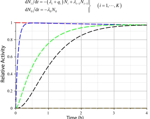
un-stable daughter products, then the sequence of decays, as denoted in relation (1) is de-scribed by the Bateman rate equations [22]
(
)
1 1
0 0 0
d d 1, ,
d d
i i i i i
N t N N i K
N t N
λ λ
λ
− −
= − + =
= −
(11)
where N0 is the number of 222
Rn atoms. If the sequence is terminated at 210
Pb,
then K=5.
A general method to solve coupled linear differential equations like (11) is given in
[23]. The solution to (11) can also be expressed in iterative form [24]
( )
( 1)( )
1 0
e it te i i t d
i i
N t −λ λ λ− − ′N t t
− ′ ′
=
∫
(12)which is particularly useful for numerical solution by computer. Of relevance to the present work is the limiting case known as secular equilibrium, a steady-state condition of equal activities between a long-lived parent and much shorter-lived daughter radio-nuclides. Mathematically, the criteria for secular equilibrium are
(
)
0 0 0 1, , i i i i K N N λ λ λ λ = = .
(13)
In light of the preceding background, consider a GM detector with circular window of radius α over whose surface slowly diffuses a current density j0 of 222Rn atoms
of steady-state number density n0. Assuming azimuthal symmetry of the detector and steady-state radon density in the vicinity of the detector throughout the time of mea-surement, the differential number of alpha counts dNα in sampling time T from dN0 radon atoms in a differential volume element located at polar coordinates
( )
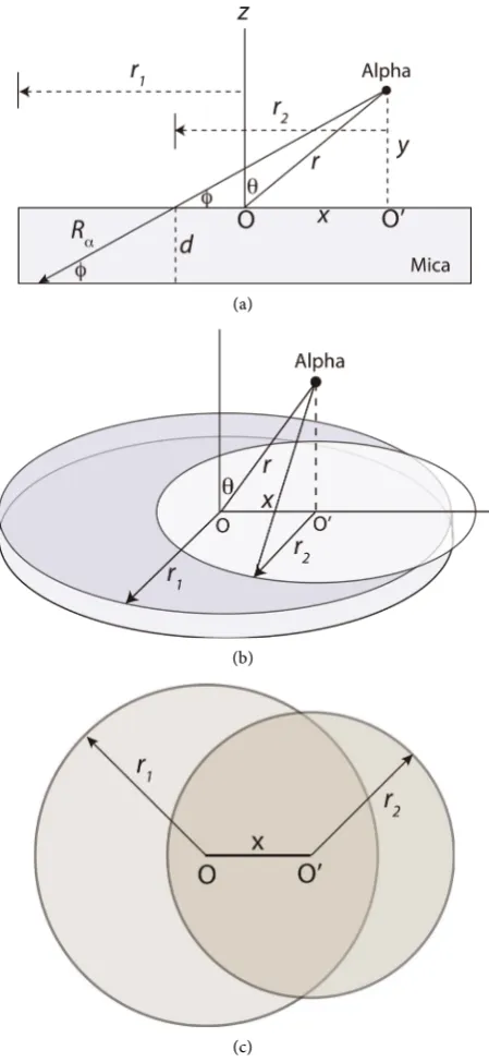
r,θrela-tive to the center of the window (Figure 1) is given by the relation
(
0 0) ( ) ( )
( )
2, ,
d d
4π π d
r E r
N T N Q r
a
α α
θ θ
δ λ Ω ε
=
(14)
in which the various factors are defined as follows:
a
δ = mean number of alpha particles from radon and its progeny contributing to
the count for each 222
Rn decay.
0
λ = decay rate of 222
Rn = 2.22 10 s× −6 −1 [25].
( )
Q r = alpha particle range function in air = fraction of alpha particles reaching a
distance r in air from their source (Figure 2).
( )
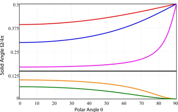
r,θΩ = solid angle of the GM window subtended at the point of alpha emission
(Figure 1, Figure 3).
( )
,E rθ = alpha transmission function = surface area of the GM window through
which an alpha particle can penetrate to the interior fill gas (Figures 4(a)-(c)).
d
ε = intrinsic alpha particle detection efficiency (for energy ≥ 4 Mev). Under
Figure 1. Azimuthally symmetric detection geometry. A radon atom located at coordinates
( )
r,θ decays, producing an alpha particle that reaches the detector window of radius α if [image:8.595.252.499.319.452.2]emitted within solid angle Ω.
Figure 2. 222
Rn 5.5 MeV alpha particle range function (in air), Equation (41).
[image:8.595.226.521.476.661.2](a)
(b)
[image:9.595.261.486.68.556.2](c)
Figure 4. (a) Geometry of transmission of alpha particle through mica window of radius α and thickness d. The alpha, emitted at point
( )
x y, relative to the vertical symmetry axis (z) of thewindow, must impact the window at angle ≥ϕ to the surface into order to pass through the mica along a path ≤ range ( )m
Rα ; (b) a line at constant ϕ rotated about the vertical axis through
O′ generates a circle of radius r2; (c) the lenticular intersection (dark gray) of this circle with
the circular mica window of radius r1=a is the region of alpha transmission.
Explicit expressions for the functions Q r
( )
, Ω( )
r,θ , and E r( )
,θ will be given inEffective detection volume (in the half space z≥0 above the GM window):
( )
2( )
π 2 2π 2( )
0
0 0 0 0
d d sin d d 2π d
d z
V Q r V r Q r r θ θ ϕ r Q r r
∞ ∞
>
=
∫∫∫
=∫
∫
∫
=∫
. (15)Effective cross section of radon flow through surface Σ normal to the GM window
surface:
( )
( )
2π( )
0
0 0
d d d 2π d
d
A Q r Q r r r ϕ rQ r r
∞ ∞
Σ
=
∫∫
Σ =∫
∫
=∫
.(16)
The upper limit to the radial integrals (15) and (16) is given as ∞, although in prin-ciple it can not exceed the dimensions of the room. Operationally, the function Q r
( )
,which takes the form illustrated in Figure 2, constrains the upper limit to a size com-parable to the alpha range in air ( )a
Rα .
The overall efficiency
ε
of the detection process is given by the range-weighted vo-lume average of the product of the fractional quantities Ω( )
r,θ 4π and E r( )
,θ
πa2( )
( )
( )
( )
π 2 2 2 0 0 2 0 , ,2π d sin d
4π π
2π d
d
r E r r Q r r
a
r Q r r
θ θ
θ θ ε ε
∞
∞
Ω
=
∫
∫
∫
. (17)Thus, the volume average of Equation (14) takes the much simplified form
0 0
dNα =εδ λα TV Ndd . (18)
The number dN0 of radon atoms diffusing over the detector window through cross section Ad in time dt is given by
0 0
dN = j A tdd (19)
where the radon current density
0 0 0
j =v n (20)
is the product of the diffusion velocity v0 and radon atomic density n0. Equation (20) and explicit expressions for v0
0 0 0
v = D
λ
(21)and a characteristic diffusion length ξ0
0 D0 0
ξ
=λ
(22)are obtained from solution of the diffusion equation based on Fick’s law [27] with im-plementation of appropriate boundary conditions. This analysis is given in Appendix 1 for the one-dimensional case in which radon diffuses toward the detector from one wall. The experimental radon diffusion coefficient in air is [28][29]
(
)
5 20 1.1 0.1 10 m s
D = ± × − . (23)
The diffusion of radon over the detector results in an effective residence time in the detection volume
r d 0 d t V v A
analogous to the residence time in radioactive flow measurements [30] such as em-ployed in high-performance radioactive liquid chromatography [31]. The principal dif-ferences between standard methods of radioactive flow measurement and the novel GM method of radon measurement reported here are: (A) in the former the detection vo-lume is fixed by the design of the apparatus, the flow rate is a deterministic variable ad-justable by the experimenter, and a finite sample of radioactive material is used, whe-reas (B) in the latter the detection volume is determined by the energy-dependent range of the alpha particle, the flow rate is a stochastic variable determined by the diffusion of radon in air, and the quantity of radioactive material is likewise a stochastic variable determined by the duration of sampling.
Substitution of Equations ((21) and (24)) into Equation (18) leads to the compact expression
(
0)
r
d
d
d
X V T
N N
C
t T t
α
α α
α
εδ
≡ = =
∆ (25)
where Cα is the observed alpha count rate, and the radon activity per unit of volume (activity concentration) is
0 0 0
X =λ n . (26)
Inversion of Equation (26) therefore yields the sought-for radon activity concentra-tion (e.g. in Bq/m3)
r 0
d C t X
V T
α
α
εδ ∆
= . (27)
The bracketed product in the numerator of Equation (25) yields a dimensionless quantity, the number of radon disintegrations that occur in a time interval given by the residence time in the denominator. In other words, under conditions of 100% detection efficiency
(
ε=1)
and alpha emission from radon only(
δα =1)
, the number ofal-phas counted during time T would equal the actual number of radon disintegrations in the detection volume during time ∆tr.
2.3. Alpha Emission from Radon Progeny
Derivation of the activity concentration relation (27) assumed (a) effectively equivalent ranges for the three alphas produced by radon and polonium decays and (b) secular equilibrium among radon and its progeny. Examination of these two assumptions will lead to an extension of relation (27).
Consider assumption (a) first. The energy of an alpha particle determines its range and therefore the effective range function Q r
( )
, detection volume (15), flux crosssec-tion (16), GM window transmission funcsec-tion E r
( )
,θ , and detection efficiency (17).Assuming a stationary-state condition, although not necessarily secular equilibrium (to be examined next), among radon and its progeny, the analysis leading to Equation (25) can be extended to yield
0 0 0 1 1 1 2 2 2 0
0 1 2
N f V f V f V
C X T
T t t t
α
α α
ε ε ε
δ
≡ = + +
∆ ∆ ∆
where indices j=0,1, 2 respectively refer to alpha particles from 222Rn, 218
Po,
214
Po. The functions εjVj ∆tj are calculated according to the expressions given in
the previous section (and sections to follow) with insertion of the appropriate alpha range ( )a
j
R for air and R( )jm for mica in the associated range function Qj
( )
r andtransmission function Ej
( )
r,θ . The fractions fj, which sum to unity, give therela-tive proportions and effecrela-tive alpha number
1
1 4 1 4
1 0 2 0 0
0 0 0 0
, , 1
f = f f = f δα = + + = f−
(29)
of the activities
(
218)
1 Po and
(
214)
4 Po in the equilibrium mixture within the detection volume. Note that the subscript i on the activity symbol i corresponds to the progenynumber (and not the alpha particle label j) in the sequence (1) of daughter nuclides of 222
[image:12.595.194.555.537.605.2]Rn.
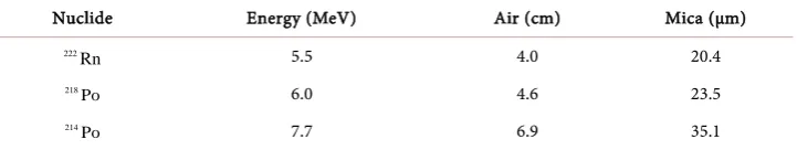
Table 1 summarizes the energies and ranges of the three alphas that potentially con-tribute to the GM count from decays of 222
Rn, 218
Po, and 214
Po.
The ranges in air and mica, calculated from Equations ((2) and (8)) respectively, in-crease approximately as the 3/2 power of alpha energy.
It is important to bear in mind that the three residence times
0
j j j
t V v A
∆ = (30)
still depend on the diffusion velocity v0 of 222
Rn. Table 2 summarizes the diffusion
properties of the three alpha-emitting nuclides with diffusion coefficients D taken from Reference [32]. Only radon has a macroscopic characteristic diffusion length on the order of meters compared with the diffusion lengths of the two polonium progeny, which are on the order of a few centimeters and nanometers, respectively. Thus, in the flow Equation (19) only radon, and not its progeny, reach the detector from points of origin well outside the alpha detection volume, a distance of at least 1 m from the walls. (Note: a number in parentheses in Table 2 signifies a power of 10.)
Consider next assumption (b) regarding secular equilibrium, expressed by relation (13). Solution (12) of the Bateman equation (11) for a closed system of radon and its
Table 1. Alpha particle energy and mean range.
Nuclide Energy (MeV) Air (cm) Mica (μm)
222
Rn 5.5 4.0 20.4
218
Po 6.0 4.6 23.5
214
[image:12.595.194.554.636.704.2]Po 7.7 6.9 35.1
Table 2. Diffusion properties of radon and alpha emitting progeny.
Nuclide λ (s−1) D (m2/s)
v= Dλ (m/s) ξ= Dλ (m)
222
Rn 2.1 (-6) 1.1 (-5) 4.8 (-6) 2.3
218
Po 3.8 (-3) 5.3 (-6) 1.4 (-4) 3.7 (-2)
214
progeny leads to the results displayed graphically in Figure 5. As seen in the figure, se-cular equilibrium is established within about 4 hours, except for 210
Pb whose activity
remains close to 0 over sampling times short in comparison to its half-life of 22 years. Under conditions of secular equilibrium, the three alpha-emitting nuclides in the decay sequence from 222
Rn to 210
Pb have the same activity, and it follows from (29) that 0 1 2 1 3
3
f f f
α
δ
= = =
= (SECULAR EQUILIBRIUM).
(31)
Depending on environmental conditions (e.g. relative humidity, temperature, aerosol content, and other factors), the radon progeny, whether initially charged or neutral, are subject shortly after generation to physical and chemical interactions with the surfaces of a room as well as with particles and molecules within the room’s atmosphere. Be-cause of these interactions, the daughter nuclides—in particular 218
Po, 214Pb, 214Bi
—can deposit (“plate out”) on solid surfaces or become part of airborne molecular clusters [33]. The resulting equilibrium activities and equilibrium alpha number δα
can therefore differ from the values (31) for secular equilibrium. Note, however, that, since 214
Po decays nearly instantly, it has the same activity as its progenitor 214Bi.
In place of the Bateman equations, the new equilibrium conditions can be deter-mined from solution of the Jacobi equations [34][35], which in their simplest form for a closed, unventilated room with clean air (corresponding to experimental conditions in this paper), become
(
)
1 1(
)
0 0 0
d d
1, ,
d d
i i i i i i
N t q N N
i K
N t N
λ λ
λ
− −
= − + + =
[image:13.595.222.529.389.633.2]= − (32)
Figure 5. Evolution in time of the ratio of activities of 222
Rn and progeny to the activity of
222
Rn at t=0 : 222
Rn (red), 218Po (blue), 214
Pb (green), 214
Bi and 214Po (black),
210
Pb (brown). Secular equilibrium is achieved in about 4 hours, except for 210
Pb whose half-life is 22.3 y. The activity of 214
Po, whose half-life is 165 μs, is practically identical to that of its progenitor, 214
where
(
)
i i
q =v S V (33)
is the loss rate, vi is termed the deposition velocity, and S V is the surface to vo-lume ratio of the room. The equilibrium progeny activities i relative to the activity of radon 0 obtained from the steady-state solution to Equation (32) are given by
1 0 1 1 i k i k k q λ − = = +
∏
. (34)
In the experimental section of this paper indoor radon activity concentrations are reported for measurements taken in an unventilated basement room with cement block walls and very low dust and aerosol content in the air. Progeny resulting from radon decay are more likely to become part of air molecular clusters than to plate out. Expe-rimental values for the deposition velocity of attached radon progeny have been found experimentally to range from about 0.03 to 0.20 m/h [36]. To estimate the most un-biased distribution of a physical variable consistent with known information, statistical physicists employ the principle of maximum entropy (PME) [37] [38]. Given only the range
(
v v1, 2) (
= 0.03, 0.20)
of the deposition velocity, the PME leads to a uniformdistribution with respective mean and variance
(
1 2)
2 1
2 0.115 m h 12 0.049 m h
v v v v
v v
σ
= + =
= − = (35)
which is in excellent accord with the value 0.0117 m/h obtained from a recent statistical fit to data taken in indoor dwellings [39].
Substitution of v=0.115 m hand the value S V 2.08 m= −1 (for the room in which
measurements were made) into Equations ((33) and (34)) leads to equilibrium activity ratios
3 4
1 2
0 0 0
0.98, 0.85, = 0.77
= = =
(36)
from which follow the equilibrium proportions and number of alpha particles per ra-don decay
0 1 2
1 4 0 0
0.364, 0.358, 0.278
1 2.75
f f f
α δ = = = = + + =
(JACOBI EQUILIBRIUM).
(37)
Inversion of Equation (28) then yields the general operational relation for radon ac-tivity concentration measured with two GM counters in sampling time T
1 0 0 0 1 1 1 2 2 2 0
0 1 2
C f V f V f V X
T t t t
α
α
ε ε ε
δ
−
= ∆ + ∆ + ∆
.
(38)
(
0)
331.204 pCi L cpm 44.55 Bq m cpm Jacobi Equilibrium 1.089 pCi L cpm 40.29 Bq m cpm Secular Equilibrium Kα ≡ X Cα = =
=
.(39)
To good approximation, the standard deviation of activity (38) is then
0
X Kα Cα
σ = σ (40)
in which the uncertainty σCα in alpha count rate is governed by Poisson-Gauss
statis-tics. (Note: The characteristic feature of Poisson statistics is that the variance σ2 equals the mean µ. For a mean count µ ≥ ~ 10 per sampling interval, the Poisson
distribution is adequately represented by a Gaussian distribution with σ2 =µ.)
It is to be noted explicitly that relation (39) does not depend on a non-calculable em-pirical proportionality constant that must be determined independently by calibration against a primary standard. Rather, the physical quantities whose numerical values en-ter Equation (38) are measurable properties of particles (e.g. alphas), maen-terials (e.g. mica), and local environment (e.g. air). As such, the more accurately these physical quantities are known for the conditions under which measurements are made, the bet-ter will be the resulting estimate of radon activity concentration. Nevertheless, the nu-merical values in relation (39) show that, for moderate levels of radon in an unventi-lated room with clean air, the analysis based on Equation (28) with equilibrium values (37) gives results comparable to the analysis which assumed secular equilibrium values (31).
2.4. Alpha Range Function Q(r)
Figure 2 shows a nearly identical theoretical replica of the experimental transmissivi-ty—i.e. fraction of particles that pass through an absorbing medium as a function of thickness—of a 222
Rn 5.5 MeV alpha particle in air [40]. The probability of
transmis-sion is essentially 100% until the alpha particle has slowed sufficiently to generate a very large number of ion pairs and thereby rapidly come to rest. The narrow variation of al-pha ranges about the mean range (defined at 50% transmission) follows a normal dis-tribution [41] with relative uncertainty of about 5% [42]. The overall shape of the em-pirical range function closely resembles the occupation probability function of a Fer-mi-Dirac particle [43], and can be accurately represented by an expression of the form
( )
( )a1 1
e 1
r R
Q r α
κ
−
−
= +
(41)
where ( )a
Rα is the alpha mean range parameter calculable from Equation (2) for air
(and Equation (3) for mica), and
κ
is a fall-off parameter that fits the experimental transmissivity curve. The ranges of the three alpha particles are summarized in Table 1. For all three range functions in air, the value κ=28 provides a satisfactory match.2.5. Solid Angle
Ω ,θ
( )
r
Subtended by the Detector Window
is ordinarily defined only for configurations with a point-like or planar source symme-trically located on or about the symmetry axis normal to the detecting surface [44]. Such configurations do not apply to the measurement of alpha particles emitted by ra-don and polonium atoms located randomly with respect to the detector in a three- dimensional volume. For this configuration a more general relation is needed.
Figure 1 shows a radon atom at arbitrary radial distance r from the center of the azimuthally symmetric GM window and at polar angle θ to the vertical symmetry axis of the window. Of the 4π steradians into which the atom can emit an alpha
par-ticle, only the shaded portion Ω of the unit sphere centered on the atom permits the
alpha to arrive at the window surface. From basic geometry, the fraction Ω 4π of the
surface of the unit sphere is given by
(
)
1 1 cos
4π 2 ω
Ω
= − (42)
where, from Figure 1, the conical half-angle of Ω subtended at the center of the unit
sphere is
(
)
2ω= α β+ . (43)
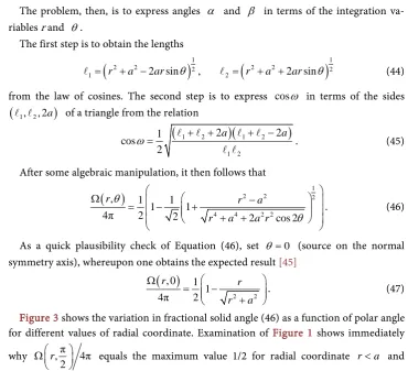
The problem, then, is to express angles
α
and β in terms of the integration va-riables r and θ.The first step is to obtain the lengths
(
)
1(
)
12 2 2 2 2 2
1= r +a −2arsinθ , 2= r +a +2arsinθ
(44)
from the law of cosines. The second step is to express cos
ω
in terms of the sides(
1, 2, 2a)
of a triangle from the relation(
1 2)(
1 2)
1 2
2 2
1 cos
2
a a
ω= + + + −
. (45) After some algebraic manipulation, it then follows that
( )
2 2 124 4 2 2
, 1 1
1 1
4π 2 2 2 cos 2
r r a
r a a r
θ
θ
Ω = − + −
+ +
. (46)
As a quick plausibility check of Equation (46), set θ=0 (source on the normal
symmetry axis), whereupon one obtains the expected result [45]
( )
2 2
, 0 1
1
4π 2
r r
r a
Ω
= −
+
[image:16.595.185.556.324.661.2] . (47) Figure 3 shows the variation in fractional solid angle (46) as a function of polar angle for different values of radial coordinate. Examination of Figure 1 shows immediately why ,π 4π
2 r
Ω
equals the maximum value 1/2 for radial coordinate r<a and
equals 0 for r>a. The solid black line in the figure denotes the threshold value π
, 4π 2 a
2.6. Alpha Particle Transmission Function
E r
( )
,θ
Upon arrival at the surface of the GM mica window, an alpha particle will fail to pass through the mica and ionize the interior fill gas if its path length exceeds the range in mica, as given in Table 2. This constraint limits the minimum incident angle
φ
be-tween the path of the particle and the window surface to( )m
sin
φ
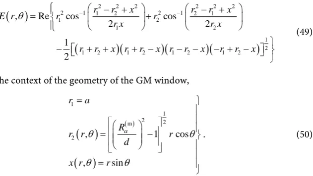
=d Rα (48) where d is the window thickness, as shown in Figure 4(a).Examination of Figure 4(a) and Figure 4(b) shows that the portion of the window surface through which an alpha can be transmitted cannot exceed the area of the circle of radius r2 from the center O′ (directly below the point of alpha emission) to the point of incidence at angle
φ
to the surface. However, depending on the location( )
r,θ of the alpha at the instant of emission, a portion of this circle can extend beyondthe area of the detector window (Figure 4(b)), which is, itself, a circle of radius r1=a with center at O. Thus, the relevant transmission area is the lenticular intersection of these two circles, shown as the dark shaded area in Figure 4(c).
The area of intersection of two circles of respective radii r1 and r2, whose centers are separated by the distance x=OO′, is readily derivable from integral calculus or from theorems of plane geometry [46] and is given by
( )
(
)(
)(
)(
)
2 2 2 2 2 2
2 1 1 2 2 1 2 1
1 2
1 2
1 2
1 2 1 2 1 2 1 2
, Re cos cos
2 2
1
2
r r x r r x
E r r r
r x r x
r r x r r x r r x r r x
θ = − − + + − − +
− + + + − − − − + −
(49)
where, in the context of the geometry of the GM window,
( )
( )( )
11 2 2 m
2 , 1 cos
, sin
r a
R
r r r
d
x r r
α
θ θ
θ θ
=
= −
=
.
(50)
The operation Re in Equation (49) to “take the real part” of the bracketed expression is necessary to include the case of non-overlapping circles. In that case, expression (49) returns 0; otherwise it can return an imaginary number if x>
(
r1+r2)
. In all other [image:17.595.237.553.373.551.2]cases, the actual area of intersection is a real positive number. The operation Re assures that the integral (17) leads to a correct real value for the overall detection efficiency.
Figure 6 shows the variation in E r1
( )
,θ for the 5.5 MeV alpha as a function of θFigure 6. Alpha transmissivity
( )
2, π
[image:18.595.208.542.310.519.2]E rθ a , Equation (49), in mica as a function of polar angle for different values of the radial coordinate (in cm) of the emission point: 2.0 (red), 1.0 (blue), 0.8 (green), 0.6 (violet), 0.4 (orange), 0.2 (plum).
Figure 7. Radial dependence of factors contributing to detection efficiency of 222
Rn 5.5 MeV alpha emitted from a point source on the normal symmetry axis. (a) alpha transmissivity
( )
2,0 π
E r a in mica (blue); (b) solid angle Ω
( )
r,0 4π (red); (c) efficiency( ) ( )
2 2,0 ,0 4π
r E r a
Ω (dashed black); (d) integrated efficiency
(
2 2)
1( ) ( )
4πa − Ω r,θ E r,θ sin dθ θ
∫
(violet).2.7. Alpha Particle Detection Efficiency
Figure 7 shows the variation with distance r from the center of the mica window of various functions contributing to detection efficiency of a 5.5 MeV alpha emitted at r on the vertical symmetry axis of the window (i.e. standard configuration for many beam experiments). Plot 7a (solid blue) depicts the transmissivity
( )
21 , 0 π
transmissible through the entire window surface. For decreasing distances below about 0.8 cm, the area of transmission rapidly falls toward 0. This effect is purely geometric. The circular area of alpha transmissibility may be thought of as the base of a cone of height r and fixed apex angle complementary to
φ
, Equation (48), as shown in Figure 4(a) & Figure 4(b). As the point of alpha emission (i.e. the apex of the cone) ap-proaches the window surface (i.e. r→0), the area of the base decreases as r2. Plot 7b (solid red) depicts the solid angle Ω( )
r, 0 4π subtended at the detector. The behavioris effectively opposite that of the transmissivity, achieving its maximum value of 0.5 for alphas emitted directly at the window surface and monotonically dropping to 0 with increasing separation. The product of the two functions
( ) ( )
2 21
, 0 , 0 4π
r E r a
Ω yields
the detection efficiency of the alpha from a point source, which is seen in plot 7c (dashed black) to reach a maximum of about 32% for a source separation of approx-imately 0.8 cm. Finally, plot 7d (solid violet) shows the directionally integrated effi-ciency
( )
π2( )
1( )
1 0 2
, ,
sin d
4π π
r E r
r
a
θ θ
ε = Ω θ θ
∫
, (51)which peaks at about 15% at a source separation of 1.13 cm.
The overall detection efficiencies of the individual 5.5, 6.0 and 7.7 MeV alpha par-ticles arriving at the detector from anywhere within the half-space above the GM win-dow are obtained by substitution in Equation (17) of the respective range functions to yield
(
)
(
)
(
)
0
1
2
5.5 Mev 0.057
6.0 Mev 0.048
7.7 Mev 0.025
ε ε ε
=
=
=
. (52)
The mean alpha detection efficiencies under conditions of secular equilibrium (31) and Jacobi equilibrium (37) are
(
)
SE 0 1 2 JE 0 0 1 1 2 2
3 0.043
0.045
f f f
ε ε ε ε
ε ε ε ε
= + + =
= + + = , (53)
which agree closely with the empirically determined alpha efficiency 4.2% provided by the manufacturer of the author’s GM counters [47].
3. Short-Term and Long-Term Measurements
of Indoor Radon Concentration
A comparison of the GM method with a commercial radon monitor to measure short- term and long-term indoor radon concentrations was made by means of two Inspector Radiation Alert detectors (to be referred to as GM1 and GM2) manufactured by S.E. International Inc (SEI), each with a halogen-quenched, pancake-style GM tube with mica window of areal density ~2.0 mg/cm2 and effective window diameter 4.5 cm. The
manufacturer-specified accuracy (in counts per minute) is cpm 10%± , tested by the
alpha particles down to 2 MeV, beta particles down to 0.16 MeV, and gamma photons down to 10 KeV. A prior (βγ)-background count of duration 192 hours showed that
GM2 was slightly more sensitive than GM1 by 1.634 0.081 cpm± , an asymmetry taken
into account in the subsequent data analysis. The GM display shows the mean count for the previous 30-second time interval, updated at intervals of 3 seconds.
The two GM counters were placed, as described in Section 2.1, on a raised (0.5 m) platform in a basement room with concrete walls, at a distance of 1.5 m from the one wall that was lower than the outside ground level due to the exterior sloping terrain. From data of radon penetration and mobility [48], it can be reasonably concluded that the main source of radon in the room was the radon flux emerging primarily from this wall. Distances to the other walls well exceeded 2 m.
On the same platform and at the same distance from the subterranean wall as the GM counters, were placed two Corentium Home radon monitors [49] to serve for comparison. The Corentium monitor performs hourly samplings of radon through a passive diffusion chamber by means of alpha spectrometry with a silicon photodiode. The sensitivity of the instrument claimed by the manufacturer is 5.55 counts per hour (cph) per pCi/L, or, equivalently, a relative uncertainty of 20% at 100 Bq/m3 after 7
days. As pointed out in Section 1, the relative uncertainty (ratio of standard deviation to mean) of a 24-hour measurement would then be about 53%. The monitor displays three readings, the mean radon activity concentration of the preceding (a) 24 hours, (b) 7 days, and (c) period up to 1 year. The measurement durations of relevance to the ex-periment reported here are 24 hours and 30 days.
Figure 8 displays graphically the sequence of 24-hour radon measurements made over a period of 30 days by (a) the method using two GM counters (red) with radon ac-tivity calculated by Equations ((37) and (38)), (b) Corentium monitor No. 1 referred to as COR1 (blue), (c) Corentium monitor No. 2 referred to as COR2 (green), and the mean value of the two Corentium readings referred to as ACOR (black). For radon ac-tivities of about 100 Bq/m3 (or 2.7 pCi/L), GM1 recorded about 62,300
(
β γ,)
countsand GM2 recorded about 67,800
(
α β γ, ,)
counts in 24 h, resulting in a net alphacount rate of approximately 2.19 0.26 cpm± in basic agreement with relation (39).
The algorithms for calculating the alpha count rate (cpm) and associated uncertainty from the raw data are given in Appendix 2. A complete tabulation of the GM and COR data is given in Table 3.
As Figure 8 shows, the radon concentrations measured by GM fall close to the center of the wide ACOR error bars in nearly every sample except the first when COR1 and COR2 were initially put into service and significantly underestimated the radon level in the room. This is a feature acknowledged by the manufacturer, who markets the Coren-tium monitor as useful primarily for sample periods well in excess of 48 h, and preferably at least 7 days. It is to be noted, therefore, that the 24 h measurements of COR1 and COR2 often varied to a greater extent between each other than each did with the GM measure-ment. The relative uncertainty of a 24 h GM-measured radon concentration is approx-imately
(
∆X X)
GM ≈0.12 at 100 Bq/m3, in comparison with
(
)
ACOR 0.37
X X
Figure 8. Sequence of 24-hour measurements of radon activity by GM method (red), commercial monitor COR1 (blue), commercial monitor COR2 (green), mean value ACOR of the two com-mercial monitors (black). The standard deviation of radon activity concentrations by (a) GM is approximately 0.32 pCi/L, (b) commercial monitor ranges from about 0.90 to 1.44.
the mean reading of COR1 and COR2.
The method to measure radon concentration with GM counters, although especially useful for short-term (24 h) sample periods, also provides accurate long-term radon le-vels with an uncertainty that decreases with the square root of sampling time. From the data in Table 3 one can calculate the mean radon concentration over the 30-day sam-pling period for each modality (GM vs commercial monitor):
( ) ( )
( ) ( )
GM GM
0 0
ACOR ACOR
0 0
3.04 0.06 pCi L 2.94 0.21 pCi L X
X
σ σ
± = ±
± = ± .
(54)
The results (54) show that, with respect to the Corentium monitors which are mar-keted as a standard for radon testing, the proposed GM-based method yielded a statis-tically equivalent mean long-term value of radon concentration. Assuming that the two sets of measurements are samples from normal distributions, the statistic z for testing the equivalence of two means [50]
( ) ( )
( )
(
)
(
( ))
ACOR GM
0 0
2 2 2 2
ACOR GM
0 0
2.94 3.04
0.458
0.21 0.06
X X
z
σ σ
− −
= = =
+ +
(55)
is itself normally distributed as N
( )
0,1 —i.e. as a standard normal variate of 0 meanand unit variance. It then follows that the probability that a subsequent series of GM measurements would yield a value greater or lesser than twice the observed value in (55) (that is, two standard deviations from the mean difference of 0) is
2
2 2
2
1
1 e d 36.0%
2π
z u z
p= − − − u=
∫
. (56)oc-curred through pure chance is 5%. Since probability (56) well exceeds the 5% threshold, the difference between the two means in (54) is regarded as statistically insignificant. It
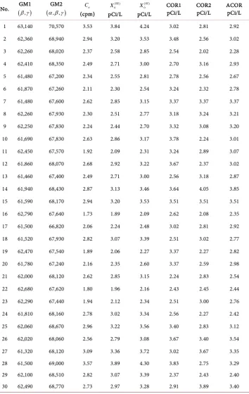
Table 3. GM counts and radon activity (24 h sampling over 30 days).
No. (GM1 β γ, ) (α β γGM2 , , ) Cα
(cpm)
( )SE 0
X
pCi/L
( )JE 0
X
pCi/L
COR1
pCi/L COR2 pCi/L ACOR pCi/L
1 63,140 70,570 3.53 3.84 4.24 3.02 2.81 2.92 2 62,360 68,940 2.94 3.20 3.53 3.48 2.56 3.02 3 62,260 68,020 2.37 2.58 2.85 2.54 2.02 2.28 4 62,410 68,350 2.49 2.71 3.00 2.70 3.16 2.93 5 61,480 67,200 2.34 2.55 2.81 2.78 2.56 2.67 6 61,870 67,260 2.11 2.30 2.54 3.24 2.32 2.78 7 61,480 67,600 2.62 2.85 3.15 3.37 3.37 3.37 8 62,260 67,930 2.30 2.51 2.77 3.18 3.24 3.21 9 62,250 67,830 2.24 2.44 2.70 3.32 3.08 3.20 10 61,690 67,830 2.63 2.86 3.17 3.78 2.24 3.01 11 62,450 67,570 1.92 2.09 2.31 3.24 2.89 3.07 12 61,860 68,070 2.68 2.92 3.22 3.67 2.37 3.02 13 61,460 67,400 2.49 2.71 3.00 2.56 3.18 2.87 14 61,940 68,430 2.87 3.13 3.46 3.64 4.05 3.85 15 61,590 68,170 2.94 3.20 3.53 3.51 3.51 3.51 16 62,790 67,640 1.73 1.89 2.09 2.62 2.08 2.35 17 61,500 66,820 2.06 2.24 2.48 3.02 2.81 2.92 18 61,520 67,930 2.82 3.07 3.39 2.51 3.02 2.77 19 62,470 67,540 1.89 2.06 2.27 3.37 2.27 2.82 20 61,780 67,240 2.16 2.35 2.60 3.37 2.59 2.98 21 62,000 68,120 2.62 2.85 3.15 2.24 2.83 2.54 22 62,680 67,620 1.80 1.96 2.16 2.43 2.45 2.44 23 62,290 67,440 1.94 2.12 2.34 2.51 3.00 2.76 24 61,810 68,160 2.78 3.02 3.34 2.56 2.27 2.42 25 62,060 68,670 2.96 3.22 3.56 3.40 2.83 3.12 26 62,020 68,060 2.56 2.79 3.08 3.67 3.40 3.54 27 61,320 68,120 3.09 3.36 3.72 3.02 3.67 3.35 28 61,500 69,000 3.57 3.89 4.30 3.83 2.75 3.29 29 62,100 68,510 2.82 3.07 3.39 2.37 2.43 2.40 30 62,490 68,770 2.73 2.97 3.28 2.91 3.89 3.40
is worth emphasizing, however, that the difference of the two mean long-term mea-surements in (54) would be statistically significant if those two concentrations were both measured by the GM method. In that case, the relevant statistic would be
(
)
GM
2
2.94 3.04 1.18 2 0.06
z = − =
(57)
with associated p-value
2 GM
GM
2 2
GM 2
1
1 e d 1.84%
2π
z u z
p = − − − u=
∫
(58) [image:23.595.223.549.113.207.2] [image:23.595.196.555.462.665.2]which is considerably below the 5% threshold of significance. The reason for the dif-ference in outcomes between (56) and (58) is due to the much lower standard error of the GM measurements in comparison to measurements by the commercial monitor. This seminal point is elucidated further in Figure 9.
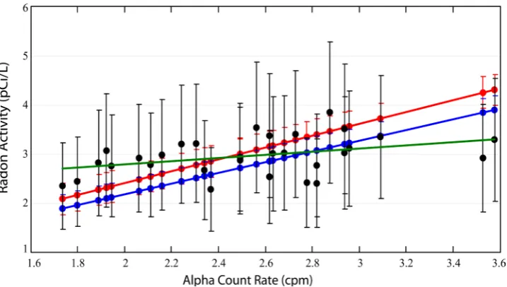
Figure 9 shows a plot of the ACOR (24 h) radon concentrations (black points) as a function of the corresponding GM-measured alpha count rate. Superposed on the plot is the linear relation (38) for conditions of secular equilibrium (blue) and Jacobi equili-brium (red). The slopes of the two lines, given by expression (39), fall within the error bars (±1 standard deviation) of the commercial monitor. Also superposed is the
maximum-likelihood (ML) line of regression [51] (green) to the ACOR measurements with slope 0.32±0.76, which signifies statistically a flat line, although a slight rise of
the data points with increasing alpha cpm values is marginally visible if the points near 3.6 cpm are disregarded. Assuming that the measurements of the commercial monitor comprise a linear trend with normally distributed random noise, one can interpret
Figure 9 in the following heuristic way. In the limit of numerous 24 h measurements, the accumulation of black points along each vertical line of constant alpha cpm would
be distributed with a Gaussian density centered on the intersecting theoretical red or blue line (depending on equilibrium conditions) given by Equation (38). One can infer from the figure that many such points would be required before the ML line of regres-sion to the radon concentration estimated by commercial monitor would be statistically equivalent to theoretical relation (38) of the GM method.
The GM counters and commercial radon monitors used in this experimental com-parison both sampled environmental radon through a process of passive diffusion. One may inquire, therefore, why it is that the GM method can make consistent short-term measurements with much lower statistical uncertainty, whereas short-term measure-ments of the commercial monitor show wide scatter and insensitivity to the total alpha count rate. An explanation, at least in part (since the programming of the commercial monitor is a proprietary secret), is that the built-in control volume according to Coren-tium is 24 cm3, whereas the effective detection volumes of the 5.5, 6.0, and 7.7 MeV
al-pha particles in open air are, according to Equation (15), about 139, 210, and 700 cm3
respectively.
4. Conclusions
In the comprehensive description of methodologies in the World Health Organization Handbook [6] for measuring indoor radon activity (summarized in Section 1), the use of GM counters is not included. Indeed, one can find explicit statements from manu-facturers of GM counters [52] that their utility for detecting (let alone actually measur-ing) radon is debatable. Reasons given or implied include (a) GM tubes do not detect radon directly; (b) GM tubes cannot determine whether a detected alpha came from radon or its progeny; (c) GM efficiency for alpha detection is low; (d) there is no fixed volume within which a radon sample can be confined and its concentration measured.
While the preceding statements are not altogether incorrect, they do not constitute valid arguments against the use of GM counters as an effective methodology to meas-ure—and not merely detect—indoor concentration of radon. The statements presup-pose the use of only a single GM counter and assume the necessity of an initially deter-mined volume of radon. As shown in this paper, neither supposition is justified.
In this paper I describe and demonstrate a method to measure indoor radon using two GM counters, which, together with the theoretical analysis derived here for con-verting an alpha count rate into a radon concentration, provides a number of advan-tages over alternative methodologies:
• The method is especially suitable for daily monitoring of radon since it provides an
activity concentration after just 24 h in situ sampling that eliminates the need to send a prepared sample to a testing laboratory. For continuous monitoring, this saves users much time and considerable expense. Other methodologies (e.g. al-pha-track counting) may have higher accuracy, but are not a convenient or eco-nomical option for researchers or home dwellers who require frequent or conti-nuous radon monitoring.
con-centrations than do commercial radon monitors employing alpha detection in a passive diffusion chamber.
• The GM method yields radon concentrations of comparable accuracy to that of
commercial monitors employing sampling by passive diffusion.
• The method employs the simplest, most versatile, and overall least expensive
radia-tion detecradia-tion instrumentaradia-tion (simply two pancake GM counters) for non-nuclear researchers and home dwellers who are not trained in nuclear spectrometry or do not have their own nuclear spectrometry instrumentation. As such, the GM method can be especially useful in geographical areas where access to specialized radon testing equipment or testing laboratories is inadequate. Or, in fact, useful in any mi-lieu for people who want to monitor indoor radon levels themselves.
The principles behind the experimental method and theoretical analysis described in this paper are physically verifiable and fully transparent (in contrast to the operation and programming of commercial monitors which are patent-protected intellectual property). The use of two monitors, so placed as to receive alpha particles only from radon and its polonium progeny, makes it possible to separate the alpha signal from the beta and gamma background. Whereas a commercial radon monitor may use energy selection to count alphas from radon only, the method described here counts alphas from both sources and uses the laws of physics and properties of materials to calculate the mean number of alphas detected per radon decay.
An essentially novel feature to the method described here is the means by which the alpha count rate is converted into a radon concentration even though there is no built-in control volume. This is accomplished by calculating an effective detection vo-lume (15), detection cross section (16), and residence time (24), which are determined by the physical laws governing alpha particle interactions in matter and the diffusion of atoms in air. Moreover, the theoretical analysis presented here can be applied to differ-ent environmdiffer-ental conditions of indoor radon measuremdiffer-ent, once the effects of these conditions on the diffusion of radon gas and the equilibrium of radon and its progeny have been ascertained.
References
[1] L’Annunziata, M.F. (1998) Handbook of Radioactivity Analysis. Academic Press, New York, 749.
[2] De Felice, P. (2007)Primary Standards of Radon. Metrologia, 44, S82-S86. http://dx.doi.org/10.1088/0026-1394/44/4/S11
[3] Bodansky, D. (1996) Nuclear Energy: Principles, Practices, and Prospects. Springer, New York, 33.
[4] Hafemeister, D. (2007) Physics of Societal Issues: Calculations on National Security, Envi-ronment, and Energy. Springer, New York, 190.
[5] A Citizen’s Guide to Radon (2012) US Environmental Protection Agency EPA-402/K- 12/002. http://www.epa.gov/radon
[7] Kumar, A. and Chauhan, R.P. (2014) Active and Passive Measurements of Radon Diffusion Coefficient from Building Construction Materials. Environmental Earth Sciences, 72, 251- 257. http://dx.doi.org/10.1007/s12665-013-2951-5
[8] Silverman, M.P. (2015) Personal Correspondence with the Corentium AS (Oslo, Norway), Manufacturer of the Corentium Digital Radon Monitor.
[9] Silverman, M.P., Strange, W., Silverman, C.R. and Lipscombe, T.C. (1999) Tests of Alpha-, Beta-, and Electron Capture Decays for Randomness. Physics Letters A, 262, 265-273. http://dx.doi.org/10.1016/S0375-9601(99)00668-4
[10] Silverman, M.P. and Strange, W. (2009) Search for Correlated Fluctuations in the β + Decay of Na-22. Europhysics Letters, 87, Article ID: 32001.
http://dx.doi.org/10.1209/0295-5075/87/32001
[11] Corentium FAQ. https://corentium.com/ca-en/product/home/
[12] Kendall, M.G. and Stuart, A. (1963) The Advanced Theory of Statistics: Vol 1: Distribution Theory. Hafner, New York, 193-195.
[13] Riley, J.A. (1996) Student Measurement of Radon Gas Concentrations. American Journal of Physics, 64, 72-77. http://dx.doi.org/10.1119/1.18295
[14] WHO Radon and Health Fact Sheet (2011)
http://www.who.int/mediacentre/factsheets/fs291/en/
[15] Bichsel, H., Groom, D.E. and Klein, S.R. (2015) Chapter 32: Passage of Particles through Matter. Particle Data Group.
http://pdg.lbl.gov/2015/reviews/rpp2015-rev-passage-particles-matter.pdf
[16] Lapp, R.E. and Andrews, H.L. (1972) Nuclear Radiation Physics. 4th Edition, Prentice-Hall, Englewood Cliffs, 198-203.
[17] Tsoulfanidis, N. and Landsberger, S. (1995) Measurement & Detection of Radiation. 2nd Edition, Taylor & Francis, Washington DC, 132-136.
[18] Schlatter, T.W. (2010) Atmospheric Composition. Encyclopedia of Aerospace Engineering. Wiley, Hoboken. http://dx.doi.org/10.1002/9780470686652.eae319
[19] Canberra GM Pancake Detectors.
http://www.canberra.com/products/detectors/pdf/Pancake-GM-SS-C37516.pdf
[20] Silverman, M.P. (2015) Search for Non-Standard Radioactive Decay Based on Distribution of Activities. Europhysics Letters, 110, Article ID: 52001.
http://dx.doi.org/10.1209/0295-5075/110/52001
[21] Silverman, M.P. (2016) Search for Anomalies in the Decay of Radioactive Mn-54. Euro-physics Letters, 114, Article ID: 62001. http://dx.doi.org/10.1209/0295-5075/114/62001 [22] Friedlander, G. and Kennedy, J.W. (1955) Nuclear and Radiochemistry. Wiley, New York,
129-137.
[23] Silverman, M.P. (2014) A Certain Uncertainty: Nature’s Random Ways. Cambridge Uni-versity Press, New York, 315-318. http://dx.doi.org/10.1017/cbo9781139507370
[24] Silverman, M.P. and Strange, W. (2004) The Distribution of Composite Measurements: How to Be Certain of the Uncertainties in What We Measure. American Journal of Physics, 72, 1-14. http://dx.doi.org/10.1119/1.1738426
[25] National Nuclear Data Center. Brookhaven National Laboratory. http://www.nndc.bnl.gov/nudat2/chartNuc.jsp