Munich Personal RePEc Archive
A new unit labour cost changes
decomposition four pillars of cost
competitiveness recovery
Peroni, Chiara and DiMaria, Charles Henri
STATEC
30 April 2012
A new unit labour cost changes decomposition
Four pillars of cost competitiveness recovery
Charles-Henri DiMaria and Chiara Peroni∗
Abstract
This article presents a new decomposition of unit labour costs into compensation per worker and labour productivity, which, in turn, is decomposed into efficiency gains, tech-nical progress and capital deepening. Data for Western European countries and the US show that the evolution of labour productivity components counteracts the deterioration in countries’ cost competitiveness caused by increases in nominal wages. The policy im-plication is that efforts aimed at reducing nominal labour costs should be accompanied by policies fostering capital deepening. Further improvements in countries’ cost compet-itiveness can be achieved by enhancing efficiency gains and technical progress, which has been mostly negative during the period under study.
KEYWORDS: unit labour cost, labour productivity, efficiency, technical change, cap-ital deepening.
Competitiveness is high on the policy agenda. The recent crisis has highlighted structural weaknesses of developed economies and re-fuelled a heated debate on the causes and reme-dies to the high unemployment and deterioration in the economic performance of Western European countries. The budgetary tightening dictated by the public debt crisis means that limited resources are available to foster economic growth; furthermore, countries belonging to a monetary union can no longer use competitive devaluation for expanding demand. Thus, for members of the Euro zone, where monetary policy is committed to price stability, unit labour costs are crucial to attain increased competitiveness (Collignon, 1999). As devaluation is no longer possible and the EU strengthens fiscal discipline, it is proposed that economic recovery should be achieved through labour market and wage bargaining adjustments (Barkbu et al., 2012). The so-called internal devaluation proposal advocates a reduction in nominal wages as essential to exit the crisis. Others question the relevance of such policy as there is no conclusive empirical evidence showing that decreases in unit labour costs lead to the growth of export shares (Felipe and Kumar, 2011).
This short article aims to clarify the link between labour costs and countries’ compet-itiveness. In particular, it examines the link between cost competitiveness (intended as a reduction in unit labour cost) and labour productivity and its determinants, and stresses that the latter are important sources of competitiveness. Unit labour costs (ULC hereafter) are defined as the ratio of total nominal cost per employee to real labour productivity. If in a given country total nominal costs per employee increase faster than labour productivity,
∗The authors work at Statec, the Institut National de la Statistique et des Etudes Economiques,
1 THE DECOMPOSITION OF UNIT LABOUR COSTS
then inflationary demand pressures may emerge and the country could lose competitiveness. Thus, ULC changes reflect the comparative evolution of total nominal costs per employee to labour productivity (e.g. Ark et al., 2005). In turn, following Kumar and Russell (2002), labour productivity changes can be decomposed into three elements: efficiency changes, tech-nical changes and capital deepening. This allows us to highlight four components of ULC, which broadens policy perspective and enriches the analysis of ULC changes. Innovation, investment in tangible and intangible capital, labour quality and business environment come into play in a formalised manner through efficiency change, technological change and capital deepening.
This article is organised as follows. The first section presents the decomposition of ULC, and gives an economic interpretation of each of its components. Then, the following sec-tion presents real data on the evolusec-tion of each term of the decomposisec-tion for 15 European countries and the United States from 1995 to 2009. The last section concludes.
1
The decomposition of Unit Labour Costs
ULC is defined as total labour compensation (TLC) per unit of output (GDP).1
Dividing each term by labour (L), ULC can be written as the ratio of compensation per employee to labour productivity:2
U LCt=
T LCt/Lt
GDPt/Lt
(1)
Changes in ULC from t to t+1 can be written as follows:
U LCt+1
U LCt =
T LCt+1/Lt+1
GDPt+1/Lt+1
T LCt/Lt
GDPt/Lt
(2)
Taking logs and rearranging terms one has:
dln(U LCt+1) =dln
T LCt+1
Lt+1
−dlnGDPt+1
Lt+1
(3)
(Here d denotes change in the logarithm from t to t+1.) The equation above shows that, in order to recover cost competitiveness, a country could decrease labour cost and/or increase labour productivity. Kumar and Russell (2002), in a framework that allows for inefficiency in production, and assuming constant returns to scales technology, show that labour productivity changes can be decomposed into efficiency changes (EFF), technical changes (TECH) and capital deepening (CAP). ULC changes can be written as follows:
dln(U LCt+1) =dln
T LCt+1
Lt+1
−ln(EF F)t+1−ln(T ECH)t+1−ln(CAP)t+1 (4)
1Whether total labour compensation is expressed in real or nominal terms, the reasoning presented in this
section remains the same.
2Ideally, a measure of ULC should be based on hours worked, especially for the purpose of international
1 THE DECOMPOSITION OF UNIT LABOUR COSTS
The equation above shows that an increase in 1% in efficiency (or any other components of labour productivity) lowers unit labour costs by about the same amount (ceteris paribus). Conversely, any percentage increase in nominal compensation per worker will increase ULC by the same amount. It should also be noted that a percent change in efficiency has the same effect than one percent change in technical progress and capital deepening on ULC. (Efficient countries, however, can only improve their ULC performance by technical change and capital deepening.)
Positive efficiency changes mean that countries moves towards best practices (the techno-logical frontier), or maximum feasible production given inputs use. This could be achieved through improvements/changes in managerial practices, firms’ decision structure and learning by doing. Such elements, under the control of the management, are among the determinants of productivity identified by Syverson (2011).3
Technical change measures technical progress, or expansions in feasible production. Tech-nical progress reflects the ability of countries to innovate, as it results from successful research and development activities. It evolves with investments in intangible capital, which measures the amount of knowledge and organisational capital and firm-specific skills. (Corrado et al., 2009, highlight that intangibles are also a determinant of the evolution of efficiency.)
The first two components of labour productivity, efficiency and technical change, deter-mine total factor productivity (TFP), which represents those productivity gains resulting from efficiency in combining inputs to production. (In other words, higher TFP means that one can produce more for any given combination of inputs.) As seen above, TFP changes reflect a complex mix of elements such as increase in knowledge from innovation, investment in intangible, organisational and managerial practises.
The last term, capital deepening, which summarises the contribution of the two inputs to production, capital and labour, has received various interpretations. Pilat (2004) explains that, when capital deepening increases, new capital is used, which introduces new technolo-gies in the production process. The most interesting explanation of capital deepening is given by Frankel (1962). This author argues that firms accumulate capital in response to market conditions and economic opportunities. As a result, capital deepening increases reflect fac-tors external to the firm that explain productivity changes, such as changes in regulatory frameworks or flexible inputs markets.
The Kumar and Russell framework has become popular in interpreting and depicting the evolution of labour productivity. Acemoglu and Guerrieri (2006) have developed a model where the engine of growth is capital deepening. Others have focused on innovation and technical progress as main determinants of growth (Romer, 1986, 1989). Empirically, it has been found that a substantial part of labour productivity growth cannot be explained by capital deepening (Fare et al., 1994).
The ULC decomposition of this section shows that increases in average compensation of workers worsen competitiveness. Conversely, countries cost competitiveness improves fol-lowing improvements in efficiency and/or the occurrence of technical change and/or capital intensity increases.
The following section analyses the evolution of components of cost competitiveness re-viewed in this section in real data, from 1995 to 2009. ULC is defined by total labour
com-3This list is clearly non-exhaustive, as other elements can affect efficiency. The adoption of ICT systems
2 RESULTS
pensation (TLC) divided by labour. It is compiled by the OECD and is expressed in PPP. Output is measured by GDP and labour by number of persons employed. GDP and em-ployment series are from the Eurostat Economy and Finance database.4 Estimates of capital
stock are constructed using capital stock data from the EUKLEMS database and investment series from Eurostat.5
The components of labour productivity are computed using Data Envelopment Analysis (DEA) assuming constant returns to scale (Fare et al., 1994). The DEA method, based on the concept of production possibility sets, evaluates the performance of each economic units (countries/industries/firms) with reference to an efficient frontier, which identifies the best-practise technology using convex combinations of observed inputs and outputs. One of the main advantages of DEA is precisely that it computes different sources of TFP growth, distinguishing the effect of efficiency changes from the effect of “pure” technical progress. Another advantage is that measures of productivity are computed by using only the available data, while making minimal assumptions on the functional form of the technology (sauf
returns to scale) or on market structure. The method, though computationally intensive, has mild data requirements and is robust to changes in the data. A brief overview of DEA, with some technical and computation details, is available in the appendix to this article.
2
Results
Table 1 shows that countries have experienced competitiveness losses from 1996 to 2009. Notably, in the aftermath of the 2007-2009 recession ULC decreased in all countries, with the exception of Luxembourg and United Kingdom.
Greece, United Kingdom and Portugal have experience the largest increase in ULC mov-ing, respectively, from a value of 100 in 1995 to 161, 148 and 143 in 2010. (Spain’s ULC growth is also high, but data is missing for the last year.) Countries with the lowest ULC are Germany (104 in 2010, assuming a value of 100 in 1995), Austria (111) and Sweden (120). The case of Germany is interesting in the light of a study of Soskice and Iversen (2001). According to these authors, in a group of countries comprising the Netherlands, Belgium, Austria and France, large companies increasingly relate their wage increases to unit labor cost developments in Germany. The correlation of the ULC evolution in those countries to the one of Germany ranges from 0.55 for France to 0.69 for Austria.
Interestingly, the countries hit by the debt crisis (Spain, Greece, Ireland and Portugal) are among those that experienced the largest growth in ULC, which seems to support the ”internal devaluation” view. Indeed, the highest deterioration in cost competitiveness occurred in Greece (3.5% average per year) followed by the UK, Spain (2.7%), Portugal (2.6%) and Ireland (2.5%). Italy’s ULC increased on average by 2.1% and, in contrast to other countries, failed to decrease during the crisis. The rise in unit labor costs in Greece, relative to the other eurozone countries, has been related to the inherent inability of the country’s trade union movement to accept real wage increases for private-sector workers in line with productivity developments (Katsimi and Moutos, 2010).
4The series have been converted using the PPP, which ensures comparability of aggregates across countries.
PPP allow researchers to express economic variables ‘as if’ they were recorded in a single common currency. This takes into account not only nominal exchange rates but also the different price levels (purchasing powers) across countries, and ensures that, for example, variables such as GDP reflect the actual size of an economy.
2 RESULTS
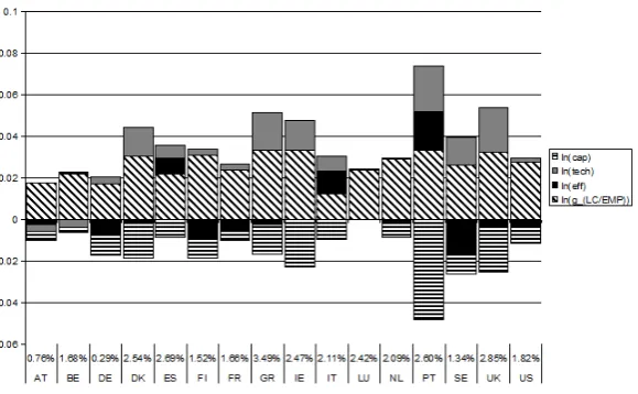
What are the main determinants of ULC increases? Table 2 shows that the largest con-tributor to the deterioration of cost competitiveness is the increase in labour compensation. This is the case for all countries. One can also see that, exception made of Spain, Greece and Italy, the growth rate of labour compensation is higher than ULC changes. This implies that the evolution of labour productivity has compensated the effects of increases in labour compensation, lowering the latter’s impact on ULC. In problematic countries, however, this has not happened and a lack in productivity improvements has resulted in an even bigger deterioration in competitiveness.
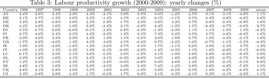
Table 3 sumarises the evolution of labour productivity in the countries analysed. One can see that labour productivity performance was weak in all countries. Its average rate of growth was barely higher than 1% in 5 european countries (Austria, Finland, Germany, Ireland and Sweden). Overall, labour productivity deteriorated in the years post-2000 and became more volatile, with the possible exception of Germany. Labour productivity declined in many countries during the recessions of 2001-2003, but this decline was more pronounced and generalised in 2008 and 2009, with all countries recording negative rates of labour productivity growth in both years.6
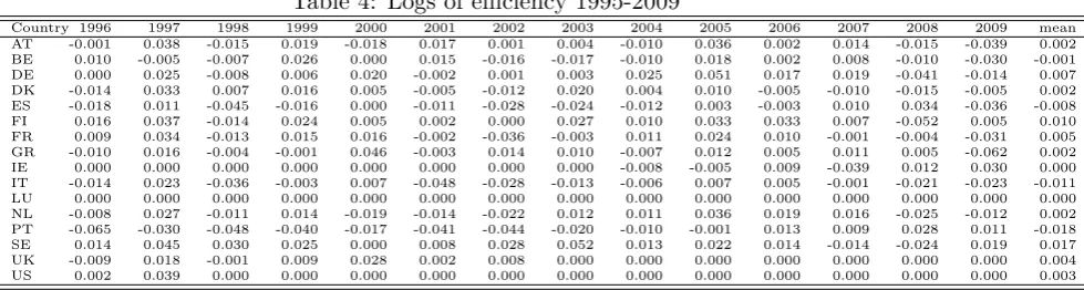
Labour productivity declined in Italy, Spain and Greece. Tables 4–6 show the evolution of the components of labour productivity, respectively efficiency changes, technical progress, and capital deepening. (Positive figures for the logarithm of efficiency change indicate that efficiency gains have occurred.)
On average, most countries have realised efficiency gains. Efficiency has decreased only in Belgium, Spain, Italy and Portugal. After realising some efficiency gains from 1995 to 1998, the US was on the frontier for the remaining of the period. The UK was on the frontier since 2003. Also Ireland made, on average, an efficient use of inputs.7
Conversely, the lack of technical progress or even technical regress, have worsened the cost competitiveness performance of nearly all countries, by not reducing ULC. Only exceptions were Austria and Belgium, whereas Luxembourg’s technical progress was absent (but, at least, not negative).
Whereas technical regress can be find in many studies at firm level (e.g. Sena, 2006), industry level (e.g. Tortosa-Ausina et al., 2012) and country level (e.g. Chen and Yu, 2012), only few authors have attempted to provide a plausible explanation of this result. For Lee and Johnson (2012), technical regress is often attributed to production issues when in fact it may result from lack of demand. Bontemps et al. (2012) emphasizes the negative effect of new regulations that generate negative technical progress. Last, for Sena (2006) it is a consequence of sharp recessions. Based on Caballero and Hammour (1994, 1996), this author argues that during recessions old techniques are substituted by new techniques. If the process of destruc-tion of old techniques is faster than the creadestruc-tion of new techniques, firms/industries/countries are experiencing technical regress. The last term, capital deepening, has improved on average for all countries and has contributed to increases the cost competitiveness (decreases in ULC).
6For detailed patterns of labour productivity and its relation with technical progress and efficiency changes,
one can see Peroni (2012).
7A zero log of efficiency means that a country is on the frontier, that is, it is making an efficient use of inputs
3 CONCLUSIONS
Figure 1: Decomposition of average ULC changes
3
Conclusions
REFERENCES REFERENCES
References
Acemoglu, D. and Guerrieri, V. (2006). Capital deepening and non-balanced economic growth. NBER working paper, N12475.
Ark, B. V., Stuivenwold, E., and Ypma, G. (2005). Unit labour costs, productivity and international competitiveness. Research Memorandum GD-80, Groningen Growth and De-velopment Centre.
Arpia, A. and Pichelmann, K. (2007). Nominal and real wage flexibility in the emu. European Economy, Economic Papers, N281.
Barkbu, B., Eichengreen, B., and Mody, A. (2012). Financial crises and the multilateral response: What the historical record shows. Journal of International Economics, Forth-coming.
Blanchard, O. (2007). Adjustment within the euro. the difficult case of portugal. Portuguese
Economic Journal, 6:1–21.
Bontemps, C., Nauges, C., Rquillart, V., and Simioni, M. (2012). Food safety regulation and firm productivity:evidence from the french food industry. TSE Working Papers 12-275, Toulouse School of Economics (TSE).
Caballero, R. and Hammour, M. (1994). The cleansing effect of recessions. American
Eco-nomic Review, 84/5:1350–1368.
Caballero, R. and Hammour, M. (1996). On the timing and efficiency of creative destruction.
The Quarterly Journal of Economics, 111/3:805–852.
Caves, D., Christensen, L., and Diewert, W. (1982). The economic theory of index numbers and the measurement of input, output, and productivity. Econometrica, 50:73–86.
Charnes, A., Cooper, W., and Rhodes, E. (1978). Measuring the efficiency of decision-making units. European Journal of Operational Research, 2:429–444.
Chen, P. and Yu, M. (2012). Total factor productivity growth and directions of technical change bias: evidence from 99 OECD and non-OECD countries. Annals of Operations Research, Online First.
Collignon, S. (1999). Unemployment,wage developments and the economic policy mix in Europe. Empirica, 26:259–269.
Corrado, C., Hulten, C., and Sichel, D. (2009). Intangible capital and US economic growth.
Review of Income & Wealth, 55:661–685.
Dubrocard, A., Ferreira, I. G., and Peroni, C. (2010). Productivite et competitivite au luxem-bourg: une comparaison par pays et par branches. Perpectives de Politique Economique, N 14, Ministere de l’economie e du commerce exterieur du Grand-Duche de Luxembourg.
REFERENCES REFERENCES
Farrell, M. (1957). The measurement of productive efficiency. Journal of the Royal Statistical
Society, Series A, 120:253–90.
Felipe, J. and Kumar, U. (2011). Unit labour costs in the eurozone: The competitiveness debate again. Levy Economics Institute, Working Paper N651.
Frankel, M. (1962). The production function in allocation and growth: a synthesis.American
Economic Review, 52:996–1022.
Katsimi, M. and Moutos, T. (2010). Emu and the greek crisis: The political-economy per-spective. European Journal of Political Economy, 26:568–576.
Kumar, S. and Russell, R. (2002). Technological change, technological catch-up, and capital deepening: relative contributions to growth and convergence. The American Economic
Review, 92:527–48.
Lee, C. and Johnson, A. (2012). Two-dimensional efficiency decomposition to measure the de-mand effect in productivity analys. European Journal of Operational Research, 216/3:584– 593.
Marx, I. (2001). Job subsidies and cuts in employers’ social security contributions: The verdict of empirical evaluation studies. International Labour Review, 140:69–83.
Milana, C. and Zeli, A. (2002). The contribution of ict to production efficiency in italy: Firm-level evidence using data envelopment analysis and econometric estimations. OECD Science, Technology and Industry Working Papers 2002/13.
Peroni, C. (2012). Productivity and competitiveness in luxemnbourg; productivity & the crisis. Perpectives de Politique Economique, N 18, Ministre de l’economie e du commerce exterieur du Grand-Duche de Luxembourg.
Pilat, D. (2004). Capital deepening, R&D and productivity - evidence from comparative studies of productivity growth. Paper prepared for conference: ”Productivity: Performance, prospects and policies”, Wellington, 28-29 July 2004.
Romer, P. (1986). Increasing returns and long-run growth. Journal of Political Economy, 94:1002–1037.
Romer, P. (1989). Capital accumulation in the theory of long-run growth. Harvard University Pres.
Sena, V. (2006). The determinant of firms’ performance: Can finance constraints improve technical efficiency? European Journal of Operational Research, 172:311–324.
Siebert, H. (1999). How competitive is europe’s labor? Kiel Working Papers, No. 927, http://hdl.handle.net/10419/22.
Soskice, D. and Iversen, T. (2001). Multiple wage bargaining systems in the single european currency area. Empirica, 28:435–456.
REFERENCES REFERENCES
[image:10.595.79.549.174.306.2]Tortosa-Ausina, E., Armero, C., and Grifell-Tatj, D. E. (2012). Bootstrapping profit change: An application to spanish banks. Computers and Operations Research, 39:1857–1871.
Table 1: Growth rates of ULC (%) 1995-2009
Country 1996 1997 1998 1999 2000 2001 2002 2003 2004 2005 2006 2007 2008 2009 mean AT -0.5% -0.2% 0.0% -0.1% 0.8% 0.2% 1.3% -0.7% 0.6% 1.0% 0.7% 3.3% 4.6% -0.6% 0.7% BE 0.2% 1.1% 1.4% 0.4% 4.2% 2.3% 1.0% -0.6% 1.4% 1.8% 2.1% 4.3% 4.3% -0.5% 1.7% DE -1.0% 0.3% 0.7% 0.5% 0.3% 0.5% 0.9% -0.4% -0.9% -2.4% -1.0% 2.2% 5.8% -1.5% 0.3% DK 1.0% 3.4% 1.9% 1.0% 4.1% 3.5% 2.1% 0.3% 1.9% 2.1% 4.4% 6.2% 4.7% -1.1% 2.5% ES 1.8% 1.8% 1.7% 2.7% 3.1% 2.8% 2.8% 2.3% 3.1% 3.1% 4.0% 4.7% 1.0% 2.7% FI -1.1% 1.3% 0.7% 0.6% 3.6% 0.8% 0.8% -0.1% 2.2% 0.3% 0.5% 5.8% 7.3% -1.5% 1.5% FR 0.2% -0.2% 0.8% 1.6% 2.2% 2.9% 2.0% 1.0% 1.8% 1.8% 1.5% 3.0% 3.1% 1.7% GR 9.2% 4.7% 2.9% 1.4% -0.7% 9.4% 1.7% 1.9% 3.5% 1.6% 3.4% 5.8% 5.4% -1.6% 3.5% IE -0.1% 5.4% 1.1% 2.7% 5.9% 0.8% 3.7% 3.9% 5.2% 3.8% 3.9% 5.0% -1.3% -5.6% 2.5% IT 2.7% -2.1% 1.5% 0.3% 3.2% 3.4% 4.0% 1.7% 3.1% 1.7% 2.2% 3.9% 3.8% 0.0% 2.1% LU -0.1% -1.0% 0.7% 2.5% 6.3% 2.2% 1.4% 1.2% 2.1% 1.2% 1.6% 6.0% 8.2% 1.7% 2.4% NL 1.0% 2.5% 1.8% 3.2% 4.5% 4.5% 2.4% 0.4% -0.3% 0.7% 1.6% 2.6% 5.1% -0.8% 2.1% PT 3.9% 3.3% 2.3% 4.3% 3.8% 3.2% 3.8% 1.0% 3.5% 0.9% 1.2% 3.4% 3.2% -1.4% 2.6% SE 0.8% 0.1% -1.2% 4.9% 5.0% 0.5% 0.5% -1.0% 0.4% -0.7% 4.1% 2.7% 4.6% -1.9% 1.3% UK 2.4% 3.9% 2.4% 2.7% 3.3% 2.1% 2.9% 1.7% 2.5% 2.5% 2.9% 2.3% 6.0% 2.2% 2.9% US 1.5% 2.8% 1.4% 3.6% 2.1% 0.3% 2.0% 1.4% 2.3% 3.0% 2.8% 2.8% 0.3% -1.0% 1.8%
Note: data are yearly changes, so that figures for 1996 reflect changes of variable from 1996 to 1997. Data is missing for Spain and France in 2009. (Sources:
[image:10.595.77.548.401.533.2]author’s calculations form Eurostat, OECD, Statec data.)
Table 2: Growth rates of labour compensation (%) 1995-2009
Country1996 1997 1998 1999 2000 2001 2002 2003 2004 2005 2006 2007 2008 2009 mean AT 2.3% 3.1% 2.9% 4.2% -2.4% 4.0% 2.1% 2.2% -0.6% 3.5% 0.9% 0.1% -0.3% 2.0% 1.7% BE 3.8% -0.2% 4.9% 5.5% 2.7% 5.7% -0.5% -0.5% 0.3% 2.2% 2.5% 0.7% 0.0% 3.1% 2.2% DE 1.7% 1.2% 3.5% 2.8% 1.2% 2.2% 3.3% 2.6% 2.2% 1.3% 1.0% -0.1% -1.3% 2.8% 1.7% DK 3.5% 4.4% 3.8% 4.8% 1.8% 5.5% 0.1% 4.6% 0.0% 3.5% 3.9% 1.4% 0.6% 4.8% 3.1% ES 2.5% 1.7% 1.1% 2.6% 1.3% 3.6% -0.6% 1.0% 0.8% 4.3% 5.1% 2.8% 2.5% 2.2% FI 2.9% 3.7% 3.2% 4.7% 1.3% 2.2% 1.2% 7.0% 2.4% 2.8% 4.2% 2.1% 0.6% 4.8% 3.1% FR 3.7% 2.1% 3.6% 4.9% 3.2% 4.4% -1.5% 3.0% 3.6% 2.5% 3.0% -1.3% -0.1% 2.4% GR 9.9% 0.1% 4.2% 5.8% 2.9% 11.9% 1.3% 2.7% 1.3% 2.6% 2.7% 4.7% 0.0% -3.5% 3.3% IE 2.4% 1.4% 0.1% 3.9% 2.8% 3.5% 4.2% 5.6% 4.1% 4.5% 7.6% -0.5% 2.4% 4.8% 3.3% IT 3.9% -0.8% 1.7% 1.7% 2.7% -2.7% 0.8% 0.4% 2.8% 2.8% 4.0% 1.6% -1.4% 0.0% 1.3% LU 2.1% 1.8% 5.7% 5.5% 1.0% 4.1% -0.4% 5.2% 0.2% 3.8% 2.1% -0.1% -0.5% 3.1% 2.4% NL 2.6% 4.1% 4.9% 6.5% 1.4% 4.2% -0.2% 5.3% 1.6% 2.6% 3.8% -0.1% -0.7% 4.5% 2.9% PT 4.4% 2.3% 5.5% 5.8% 1.6% 2.6% 3.0% 1.0% 8.0% 2.3% 3.4% 0.3% 3.1% 3.4% 3.3% SE 4.8% 1.7% 3.2% 8.7% 0.3% 2.5% 2.8% 6.2% -0.8% 2.2% 6.8% -2.3% -2.9% 3.4% 2.6% UK 5.5% 4.7% 4.4% 8.1% 4.9% 2.9% 1.9% 4.7% 1.9% 3.0% 1.5% -2.0% -0.5% 4.0% 3.2% US 4.3% 5.6% 5.7% 5.4% 1.6% 2.0% 2.9% 3.5% 2.5% 0.9% 3.1% -1.4% -2.1% 4.7% 2.8%
(Sources: author’s calculations form Eurostat, OECD, Statec data.)
Table 3: Labour productivity growth (2000-2009): yearly changes (%)
Country 1996 1997 1998 1999 2000 2001 2002 2003 2004 2005 2006 2007 2008 2009 mean AT 3.4% 2.8% 3.4% 2.9% 4.4% -3.1% 3.9% 0.8% 3.0% -1.2% 2.5% 0.1% -3.1% -4.8% 1.1% BE 2.1% 3.7% -1.3% 3.6% 5.2% -1.4% 3.5% -1.5% 0.1% -1.1% 0.5% 0.4% -3.6% -4.2% 0.6% DE 3.2% 2.8% 0.8% 2.9% 2.3% 0.9% 1.7% 2.4% 3.0% 3.2% 3.7% 2.0% -2.3% -6.9% 1.6% DK 3.2% 2.6% 1.0% 1.9% 3.9% -2.4% 2.1% -2.0% 4.4% -1.9% 1.5% -0.4% -4.7% -4.0% 0.7% ES 0.5% 0.7% 0.0% -0.6% -0.1% -1.8% 0.8% -3.3% -1.3% -2.3% 1.1% 1.1% -1.9% 1.5% -0.2% FI 2.7% 4.0% 2.4% 2.5% 4.2% -2.2% 1.3% 0.5% 7.3% 0.2% 2.5% 3.7% -3.6% -6.4% 1.6% FR 2.0% 3.6% 2.3% 2.9% 3.4% 1.0% 1.5% -3.5% 2.0% 1.8% 0.7% 1.5% -4.3% -3.1% 1.0% GR -1.7% 0.6% -4.6% 1.4% 4.5% 3.6% 2.5% -0.4% 0.7% -2.2% 1.0% -0.7% -1.1% -5.3% -0.3% IE 7.9% 2.5% -3.9% -1.0% 1.2% -3.0% 2.7% 0.5% 1.7% -1.1% 0.6% 3.8% -5.3% 3.7% 1.3% IT -1.0% 1.3% 1.3% 0.3% 1.4% -0.5% -6.0% -3.2% -1.3% -0.3% 1.1% 1.8% -2.3% -5.1% -0.9% LU 0.1% 2.2% 2.9% 5.1% 3.0% -5.2% 2.0% -1.8% 4.1% -1.9% 2.6% 0.6% -6.0% -8.4% 0.0% NL 2.9% 1.6% 1.6% 3.1% 3.4% -3.1% -0.3% -2.6% 5.0% 1.9% 2.0% 2.2% -2.7% -5.7% 0.9% PT 1.2% 0.5% -1.0% 3.3% 1.5% -2.2% -0.6% -0.8% 0.0% 4.6% 1.4% 2.3% -3.1% -0.1% 0.8% SE 4.8% 4.1% 1.6% 4.5% 3.9% -4.5% 2.0% 2.4% 7.4% -1.2% 2.9% 2.8% -4.9% -7.2% 1.5% UK 2.8% 3.1% 0.8% 2.0% 5.5% 1.6% 0.8% -1.0% 3.0% -0.5% 0.5% -1.4% -4.2% -6.3% 0.5% US 3.3% 2.8% 2.8% 4.4% 1.7% -0.5% 1.7% 0.9% 2.1% 0.3% -2.1% 0.3% -4.1% -2.4% 1.1%
[image:10.595.82.552.595.733.2]A APPENDIX: THE DEA METHOD TO MEASURE EFFICIENCY, TECHNICAL GAINS, AND PRODUCTIVITY
Table 4: Logs of efficiency 1995-2009
Country 1996 1997 1998 1999 2000 2001 2002 2003 2004 2005 2006 2007 2008 2009 mean AT -0.001 0.038 -0.015 0.019 -0.018 0.017 0.001 0.004 -0.010 0.036 0.002 0.014 -0.015 -0.039 0.002 BE 0.010 -0.005 -0.007 0.026 0.000 0.015 -0.016 -0.017 -0.010 0.018 0.002 0.008 -0.010 -0.030 -0.001 DE 0.000 0.025 -0.008 0.006 0.020 -0.002 0.001 0.003 0.025 0.051 0.017 0.019 -0.041 -0.014 0.007 DK -0.014 0.033 0.007 0.016 0.005 -0.005 -0.012 0.020 0.004 0.010 -0.005 -0.010 -0.015 -0.005 0.002 ES -0.018 0.011 -0.045 -0.016 0.000 -0.011 -0.028 -0.024 -0.012 0.003 -0.003 0.010 0.034 -0.036 -0.008 FI 0.016 0.037 -0.014 0.024 0.005 0.002 0.000 0.027 0.010 0.033 0.033 0.007 -0.052 0.005 0.010 FR 0.009 0.034 -0.013 0.015 0.016 -0.002 -0.036 -0.003 0.011 0.024 0.010 -0.001 -0.004 -0.031 0.005 GR -0.010 0.016 -0.004 -0.001 0.046 -0.003 0.014 0.010 -0.007 0.012 0.005 0.011 0.005 -0.062 0.002 IE 0.000 0.000 0.000 0.000 0.000 0.000 0.000 0.000 -0.008 -0.005 0.009 -0.039 0.012 0.030 0.000 IT -0.014 0.023 -0.036 -0.003 0.007 -0.048 -0.028 -0.013 -0.006 0.007 0.005 -0.001 -0.021 -0.023 -0.011 LU 0.000 0.000 0.000 0.000 0.000 0.000 0.000 0.000 0.000 0.000 0.000 0.000 0.000 0.000 0.000 NL -0.008 0.027 -0.011 0.014 -0.019 -0.014 -0.022 0.012 0.011 0.036 0.019 0.016 -0.025 -0.012 0.002 PT -0.065 -0.030 -0.048 -0.040 -0.017 -0.041 -0.044 -0.020 -0.010 -0.001 0.013 0.009 0.028 0.011 -0.018 SE 0.014 0.045 0.030 0.025 0.000 0.008 0.028 0.052 0.013 0.022 0.014 -0.014 -0.024 0.019 0.017 UK -0.009 0.018 -0.001 0.009 0.028 0.002 0.008 0.000 0.000 0.000 0.000 0.000 0.000 0.000 0.004 US 0.002 0.039 0.000 0.000 0.000 0.000 0.000 0.000 0.000 0.000 0.000 0.000 0.000 0.000 0.003
[image:11.595.82.573.300.432.2](Sources: author’s calculations form Eurostat, Statec data.)
Table 5: Logs of technical progress 1995-2009
Country 1996 1997 1998 1999 2000 2001 2002 2003 2004 2005 2006 2007 2008 2009 mean AT 0.022 -0.011 0.037 0.015 -0.015 0.011 0.002 0.020 -0.002 -0.014 0.001 -0.042 -0.035 0.062 0.004 BE 0.022 -0.008 0.037 0.016 -0.016 0.011 0.002 0.020 -0.001 -0.015 0.000 -0.042 -0.034 0.061 0.004 DE 0.022 -0.022 0.019 0.001 -0.026 -0.003 -0.002 0.012 -0.004 -0.018 0.000 -0.041 -0.030 0.049 -0.003 DK 0.007 -0.033 -0.001 0.001 -0.032 0.000 -0.012 -0.008 -0.017 -0.014 -0.014 -0.035 -0.048 0.019 -0.013 ES 0.022 -0.014 0.036 0.010 -0.022 0.000 -0.004 0.002 -0.013 -0.017 -0.011 -0.037 -0.031 0.059 -0.006 FI 0.022 -0.014 0.035 0.009 -0.023 -0.004 -0.006 0.005 -0.011 -0.017 -0.010 -0.034 -0.035 0.040 -0.003 FR 0.022 -0.014 0.035 0.011 -0.012 0.008 0.004 0.011 -0.005 -0.019 0.000 -0.041 -0.030 0.055 -0.002 GR -0.001 -0.031 -0.016 -0.008 -0.041 -0.001 -0.018 -0.018 -0.019 -0.012 -0.015 -0.036 -0.054 0.011 -0.018 IE 0.011 -0.035 -0.014 -0.008 -0.042 -0.010 -0.024 -0.015 -0.019 -0.014 -0.014 -0.035 -0.038 0.058 -0.014 IT 0.022 -0.019 0.027 0.005 -0.022 -0.003 -0.008 -0.004 -0.016 -0.015 -0.013 -0.034 -0.043 0.022 -0.007 LU 0.021 0.028 0.047 0.031 -0.048 0.016 -0.019 0.035 -0.015 0.023 0.007 -0.058 -0.087 0.013 0.000 NL 0.022 -0.014 0.036 0.013 -0.011 0.001 -0.004 0.008 -0.006 -0.019 -0.001 -0.041 -0.033 0.038 -0.001 PT -0.001 -0.031 -0.016 -0.016 -0.046 -0.022 -0.019 -0.007 -0.017 -0.014 -0.019 -0.035 -0.065 -0.003 -0.022 SE 0.022 -0.030 0.003 0.001 -0.033 0.002 -0.020 -0.015 -0.020 -0.013 -0.015 -0.035 -0.050 0.015 -0.013 UK -0.001 -0.031 -0.016 -0.016 -0.046 -0.022 -0.019 -0.005 -0.016 -0.011 -0.018 -0.036 -0.065 -0.001 -0.022 US 0.022 -0.019 0.027 0.007 -0.018 0.003 0.002 0.012 -0.005 -0.019 -0.007 -0.037 -0.035 0.038 -0.002
(Sources: author’s calculations form Eurostat, Statec data.)
Table 6: Logs of capital deepening 1995-2009
Country 1996 1997 1998 1999 2000 2001 2002 2003 2004 2005 2006 2007 2008 2009 mean AT 0.007 0.007 0.007 0.009 0.001 0.009 0.005 0.005 -0.001 0.003 -0.001 -0.004 0.001 0.003 0.004 BE 0.004 0.001 0.006 0.009 0.002 0.008 0.000 -0.002 0.000 0.001 0.002 -0.003 0.001 0.005 0.002 DE 0.005 0.006 0.017 0.015 0.015 0.022 0.025 0.016 0.010 0.004 0.002 -0.002 -0.001 0.007 0.010 DK 0.032 0.010 0.013 0.022 0.003 0.025 0.004 0.030 -0.006 0.019 0.015 -0.003 0.022 0.045 0.017 ES 0.003 0.002 0.002 0.005 0.004 0.019 -0.002 0.009 0.002 0.025 0.024 0.008 0.012 0.009 0.009 FI 0.001 0.001 0.004 0.007 -0.004 0.015 0.010 0.038 0.004 0.008 0.013 -0.010 0.021 0.019 0.009 FR 0.005 0.003 0.007 0.007 0.007 0.009 -0.003 0.012 0.013 0.003 0.005 -0.001 0.003 0.006 0.005 GR 0.017 -0.031 0.034 0.053 0.030 0.029 0.000 0.015 0.003 0.010 0.004 0.014 -0.005 0.031 0.014 IE 0.014 -0.005 0.004 0.020 0.011 0.036 0.029 0.032 0.016 0.025 0.042 0.018 0.062 0.016 0.023 IT 0.005 0.008 0.011 0.012 0.010 -0.011 0.004 0.004 0.019 0.019 0.027 0.012 0.011 0.001 0.009 LU 0.001 0.001 0.003 -0.001 -0.005 0.003 0.002 0.005 -0.003 0.003 -0.001 -0.004 -0.001 0.001 0.000 NL 0.002 0.003 0.005 0.007 -0.002 0.010 -0.001 0.028 0.013 0.003 0.003 -0.002 -0.001 0.026 0.007 PT 0.072 0.051 0.096 0.071 0.041 0.057 0.055 0.028 0.072 0.029 0.028 -0.006 0.036 0.041 0.048 SE 0.004 0.001 0.011 0.012 -0.014 0.010 0.016 0.035 -0.005 0.019 0.029 -0.001 -0.001 0.019 0.010 UK 0.041 0.022 0.036 0.061 0.035 0.028 0.000 0.035 0.010 0.016 0.004 -0.006 0.000 0.019 0.021 US 0.004 0.007 0.016 0.011 0.013 0.014 0.007 0.009 0.008 -0.002 0.009 -0.005 0.010 0.018 0.009
(Sources: author’s calculations form Eurostat, Statec data.)
A
Appendix: the DEA method to measure efficiency,
technical gains, and productivity
[image:11.595.80.565.477.609.2]A APPENDIX: THE DEA METHOD TO MEASURE EFFICIENCY, TECHNICAL GAINS, AND PRODUCTIVITY
measure operating efficiency by comparing observed output to the boundary of the production set (the frontier). Distance functions offer a mean of comparing different units in terms of their position to the frontier, and to study the evolution of the units’ performance when the structure of technology changes.
Assume that each economic unit — or Decision Making Unit (DMU) — produces a sin-gle output, denoted by y, using a vector of input x ∈ RN+.
8
Formally, the production possibility set in periodtis as follows:
St={(xt, yt) :xt can produce yt}; (5)
Here, The set S represents all feasible input/output vectors (x, y) such that usingxone can produce y. The boundary of S, the frontier, gives the maximum output obtainable from a given amount of inputs use. DMUs operating on the frontier are said to be efficient because they make full use of the inputs. The output distance function describes all operating DMUs in terms of their relative position to the frontier:
Dt(xt, yt) =inf{θ: (xt,yt
θ)∈St, θ ≥0}; (6)
Here,D gives the smallest (infimum) of the set of real numbers θ, where θ is such that the input/output combination (xt, yt) belongs to the production possibility set St.9 Dt(xt, yt) measures the reciprocal of the required expansion in output given inputs xt to attain the frontier defined bySt. D takes the value of 1 for those DMUs on the frontier and less than 1 for those DMUs below the frontier. Larger values ofD are associated to units closer to the frontier.
The DEA method (Charnes et al., 1978) provides a way of computing distance functions. DEA selects the most efficient unit for each observed combination of input (that is, the unit which produces the highest amount of output), and constructs the frontier by joining the set of points represented by those efficient units. This is done by solving the following linear programming problem (LP):
maxλ,Φ λ0 (7)
s.t. PJj=1xijφj ≤xi0, for every i −PJj=1yjφj+λ0y0 ≤0
Φ, λ≥0
Here, the subscripts iand j index, respectively, inputs and DMUs; Φ is a vector (J x 1) of coefficients for the DMUs; λis a score to be maximized. (The subscript 0 indicates that the problem is solved with respect to a reference DMUs.) Intuitively, the LP problem above seeks the biggest possible expansion of the output of DMU0, while remaining within the feasibility
set. The solution gives a score for each DMU, λ∗
0; the efficiency measure for DMU0 is equal
to the reciprocal of such score: E0 = 1/λ∗0. The DMUs with a score equal to 1 will define the
efficient frontier.10
8Economic units, object of the efficiency analysis, may indicate firms, industries, regions, countries. 9The terminfimumdenotes the lowest bound of the setθ.
10The formulation of problem 7, also referred to as the envelopment form, represents the dual of a non-linear
A APPENDIX: THE DEA METHOD TO MEASURE EFFICIENCY, TECHNICAL GAINS, AND PRODUCTIVITY
Clearly this method avoids the use of a tightly specified production function for which parameters should be estimated, but it is computationally intensive. Moreover, this approach does not require assumptions on the market structure (ie perfect competition), and permits different specifications of returns to scale technologies. Distance functions can also be used to construct productivity indices, as outline in the remaining of this appendix.
Caves et al. (1982) first proposed the use of the Malmquist index to measure productivity changes. Given two time period tand t+ 1, the Malmquist index of productivity is defined as follows:
Mt,t+1 =
Dt(xt+1, yt+1)
Dt(xt, yt)
Dt+1(xt+1, yt+1)
Dt+1(xt, yt)
12
; (8)
The index is given by the ratio of distance functions obtained by comparing output to inputs in time t and time t+ 1 using a given reference technology. (Here, the geometric averages of indices obtained using both St and St+1
production sets avoids the arbitrary choice of a reference technology.) In other words, equation 8 considers how much a unit could produce using the inputs available int+ 1, if it used the technology at time t, and how much a unit could produce using the inputs available int, if it used the technology available int+1.11
Fare et al. (1994) showed that equation 8 can be decomposed into efficiency gains and technical progress, as follows:
Mt,t+1 = D t+1
(xt+1
, yt+1
)
Dt(xt, yt)
| {z }
ef f iciency gains
Dt(xt+1
, yt+1
)
Dt+1(xt+1, yt+1)
Dt(xt, yt)
Dt+1(xt, yt)
12
| {z }
technical progress
; (9)
Here, the first term — a ratio of distances to the frontiers in periodtandt+ 1 — represents the pure change in efficiency. The second term, which measures the shifts in the frontier, provides a measure of technical change.12
This is achieved by comparing, for the same level of inputs (int ort+ 1), the distance functions obtained under the technology in tand t+ 1. (Once again, we have a geometric mean of ratios obtained under the technology in t and
t+ 1.)
the measurement of productive efficiency. The score formulation reduces the dimensionality of the problem as the number of constraints is equal toI (number of inputs) rather thanJ(number of DMU). The optimisation problem presented here is an output-oriented version, but it is also possible to formulate the problem as an input-oriented one. In the latter case, we seek the biggest possible reduction in inputs’ use, while keeping output levels constant.