Energy quality

Energy quality

Stern, David I.

Australian National University

19 August 2009

Online at

https://mpra.ub.uni-muenchen.de/16857/

Energy Quality

David I. Stern

Arndt-Corden Division of Economics, College of Asia and the Pacific, Australian National

University, Canberra, ACT 0200, AUSTRALIA

E-mail: [email protected]

August 2009

Abstract

This paper develops economic definitions of energy quality for individual fuels and energy

aggregates. There are both use- and exchange-value concepts as well as marginal and total

measures of energy quality. A factor augmentation or quality coefficients approach corresponds

to the use-value definition while indicators based on distance functions and relative prices are

exchange-value based definitions. These indicators are identical when the elasticity of

substitution between fuels is infinity but diverge or cannot be computed for other interfuel

elasticities of substitution. Under zero substitutability only the quality coefficients approach is

defined. I also find that the ratio of an energy volume index to aggregate joules cannot be

considered a complete indicator of aggregate energy quality as it does not account for quality

changes in the component fuels.

JEL Codes: Q40, D24, O47

1. Introduction

Not all energy sources and fuels are of equal economic productivity. These differences in

productivity are termed energy quality. Some fuels can be used for a larger number of activities

and/or for more valuable activities. For example, coal cannot be used to directly power a computer

while electricity can. The productivity of a fuel is determined in part by a complex set of attributes

unique to each fuel: physical scarcity, capacity to do useful work, energy density, cleanliness,

amenability to storage, safety, flexibility of use, cost of conversion, and so on.Fuel and energy

quality is not necessarily fixed over time as changes in technology in terms of both new techniques

of production and new products and activities change the opportunities for using fuels. However, it

is generally believed that electricity is the highest quality energy vector followed by natural gas, oil,

coal, and wood and other biomass in descending order of quality. This is supported by the typical

prices of these fuels per unit of energy, which is one way of measuring relative energy quality.

There are both biophysical and economic approaches to measuring energy quality. The leading

physical approach to energy quality is the ratio of exergy – energy that is available to perform

work – to total energy. The higher the ratio, the higher energy quality is (Cleveland et al., 2000).

But as discussed by Cleveland et al. (2000), exergy is only one property of energy sources that

affects their economic usefulness. And the exergy/energy ratio is essentially the same for all

chemical fuels and electricity. Cleveland et al. proposed fuel prices or marginal products as the

sole economic indicators of energy quality. But price is not the most fundamental definition of

energy quality and other indicators can be considered. This paper discusses alternative

definitions of economic energy quality and proposes a comprehensive set of economic

definitions and indicators.

I show that energy quality is only uniquely defined when the elasticity of substitution between

fuels is infinity – in which case all the proposed measures are equal – or zero, in which case only

one of the approaches is defined. For intermediate values of the elasticity of substitution energy

quality is a more ambiguous concept. The concept that is most relevant depends on the elasticity

of substitution and the application.

We can consider both the quality of individual fuels and the quality of an energy aggregate. Most

according to their heat content, which implicitly assumes that the different energy sources are

infinitely substitutable and of equal quality. If this is not the case, then estimates of productivity

and production relations based on these aggregates are biased. Therefore, appropriate

aggregation methods are important. The economic energy quality literature has focused on these

and conflated them with measuring quality itself (e.g. Cleveland et al., 2000; Ho and Jorgenson,

1999). This paper examines whether this interpretation is accurate.

Throughout the paper, I discuss the production case rather than the consumption case. Production

seems to be simpler to understand without the problems of wealth constraints and nonmeasurable

utility to contend with. I believe that arguments similar to those in this paper would easily

transfer into the consumption realm.

The second section of the paper reviews the various concepts in the literature that are relevant to

defining fuel quality. The third and fourth sections provide in depth definitions of the quality

coefficients and substitution approaches to measuring fuel quality. The fifth section synthesizes

these ideas and discusses when each is most relevant. The sixth section examines what a quality

adjusted aggregate energy index actually measures and the seventh section concludes.

2. Concepts of Fuel Quality

“Quality -- you know what it is, yet you don't know what it is…. But some things are

better than others, that is, they have more quality. But when you try to say what the

quality is, apart from the things that have it, it all goes poof! …... But for all practical

purposes it really does exist. What else are … grades based on? Why else would people

pay fortunes for some things and throw others in the trash pile? Obviously some things

are better than others -- but what's the "betterness"? -- So round and round you go,

spinning mental wheels and nowhere finding anyplace to get traction. What the hell is

Energy quality is easier to pin down than the concept of quality in general but still elusive. From

an economic perspective one fuel is better than another if it is more productive in producing

economic outputs or utility. The difficulty is only then in defining that productivity.

Various definitions of energy quality have been proposed and are in some cases fairly widely

used. Cleveland et al. (2000) define energy quality as "the relative economic usefulness per heat

equivalent of different fuels". In that paper, I go on to imply that the quality of individual fuels is

proportional to their marginal products and, therefore, in competitive input markets the ratio of

their prices. The rationale is that if when I substitute one fuel for another, output increases the

fuel whose quantity increases is of higher quality. Berndt (1978) just asserts that it is reasonable

to use prices as weights in constructing an index of energy, generalizing the approach suggested

by Turvey and Nobay (1965).

A similar approach is sometimes seen in the literature on labor quality (e.g. Abowd et al., 1996;

Ho and Jorgenson, 1999; Jorgenson et al., 2003). On the other hand, Kazamaki-Ottersten et al.

(1999) and Mellander (2000) define the quality of an input as a factor, which multiplies that

input, wherever it appears in the production function, while Giannis (1998) assumes that quality

adjusted labor supply is an affine function of quality. This quality factor or coefficient approach

is much more common in the literature on human capital in economic development and growth.

For example, Padilla and Mayer (2003) state that a labor quality index that multiplies the

quantity of labor is equivalent to an index of human capital. Tallman and Wang (1994) equate

labor quality with human capital per worker. Hanushek and Kimko (2000) measure labor force

quality as the average of results on international mathematics and science tests.1

Formalizing this quality coefficients approach for the special case of a production function, f,

with a single output, y, distinguishing between general factor neutral technological change, A,

and the quality factors:

y= f(A,"₁E1,...,"nEn,µ1X1,...,µmXm) (1)

1

where the "i are the quality factors of the n energy inputs Ei, and the µi are the quality factors

of the m non-energy inputs X_{i. The quality coefficients may be related to explanatory variables}

as in the labor quality literature or could be treated as latent state variables. The restriction to a

single output can be relaxed but the restriction on the form of technological change could not be

relaxed in the absence of explanatory variables that can be used to identify quality change as

something distinct from technological change.

Kander (2002) suggests that energy quality should be measured based on the use-value – in the

classical sense of the term 2 – contributed by each fuel rather than on marginal productivities or

exchange-values. She uses the usual neoclassical interpretation of the classical concept of

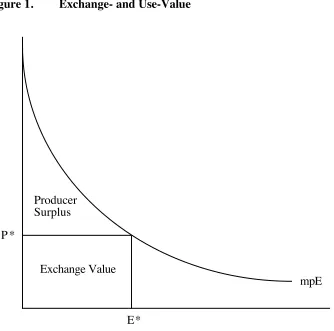
use-value as the integral of the demand curve (e.g. Hirschleifer and Hirschleifer, 1997). Figure 1

illustrates this for the producer case. mpE is the marginal product of energy. The exchange-value

is equal to P*E*. For a single input production function, the producer surplus is equal to the

profit generated. In this case the use-value generated is equal to the sum of exchange-value and

producer surplus, which is equal to total output as shown by:

"y

"EdE 0

E*

#

The idea has merit in that it tries to capture the notion that the inframarginal units of energy

contribute more to production than the marginal unit. By contrast, the marginal productivity

approach deems that any energy source that is very abundant must be of low relative quality as

the marginal units of the energy source will be used in low marginal value activities. But there

are inherent problems with integrating the area under the demand curve to derive use-value in the

multi-input case. For constant elasticity of substitution production functions, except in the case

2

in the environmental economics literature the term “use value” is confusingly used in a

of where the elasticity of substitution is infinity,3 the sum of the use-values of the individual

inputs is greater than total output and when the elasticity of substitution is less than one the

use-value of each individual input is equal to total output as each output is essential to production.4 in

the latter case there is, therefore, no way to compare the qualities of the different inputs on this

basis.

Though the usual neoclassical way of expressing the idea of use-value is to integrate the area

under the demand curve, this is not necessarily what the classical economists were thinking of

when contrasting use- and exchange-value. Based on Commons (1934), Stern (1999) explains

that for the classical economists:

“...use value was utility - the happiness or satisfaction derived from using a

commodity. The classical economists did not conceive of this utility as declining

with increasing consumption. Therefore, there was no relation between use value

per unit and the abundance or consumption of the commodity. Use value did

change with what neoclassical economists would now call changes in preferences

… The use value of a particular material object would also decline through wear

and tear over time. Commons suggested that I measure use value in physical

units…” (p473)

The quality coefficients approach achieves exactly what is stated in this quotation. Quality

coefficients are defined in terms of physical units as they multiply the quantity of each input.

Unlike the demand curve integral, they do not decline with the level of consumption. They may

increase with technological improvements and decline with depletion or depreciation. Therefore,

quality coefficients appear to correspond better to the classical concept of use-values than do

demand integrals.

3

I am referring to the traditional definition of the direct or Hicks elasticity of substitution, which takes the value of zero for the Leontief production function and infinity for the linear production function (Stern, 2009).

4

We can, therefore, approach energy quality from an exchange value approach – using relative

prices or other substitution based measures as discussed below – or a use value approach using

quality coefficients. The next two sections of the paper deal in depth with the two approaches

and following that a synthesis is laid out.

3. Quality Coefficients Approach

Quality coefficients, as introduced in equation (1), multiply each input wherever they appear in

the production function and other functions derived from it. However, there are significant

problems in actually identifying and measuring such quality changes empirically. A first problem

is to differentiate between a technological change and a change in energy quality. Take, for

example, a single input model:

y= f(A,"E) (3)

where A is technology, θ is energy quality, y is output, E is joules of energy, and f is an arbitrary

production function. How can I distinguish between A and θ? We cannot, unless I define θ in

some specific way using additional a priori information or data. The simple restriction

y=Af("E) will work if there are variable returns to scale and I use both the original production function and the first order condition to estimate the two variables A and θ.5 But this

decomposition is fairly arbitrary. There are four alternative approaches: assuming that the energy

quality of each fuel is an intrinsic factor that is constant for all time; assuming that all energy

augmenting technical change is a change in energy quality; treating energy used in different uses

as being of different qualities but assuming that that quality is fixed over time; or using

additional data to model energy quality as is done in much of the labor quality literature

referenced.

5

For example if f () is a quadratic in logarithms then the first order condition is "ln_y/_"ln_{E =#}

E +2#EE

(

)

Assuming that energy quality is an intrinsic factor that is constant for all time, is rather

unreasonable. It would mean that inventions that create new productive uses for fuels have no

influence on their perceived quality. So in this case, the relative quality of particular grades of

coal and gasoline would be considered to be the same today as it was in 1870. At the opposite

extreme, assuming that all factor-augmenting technological change associated with an input

represented changes in its quality is also seems unreasonable. Much of total TFP growth may

consist of labor augmenting technical change as is assumed in most mainstream growth models

(Acemoglu, 2000). This large gain could not surely be seen as purely representing an increase in

labor quality? A large part of the gain might for example be seen as improved management

techniques that use labor more effectively.

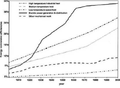
One variable that might be used to proxy energy quality is exergy conversion efficiency - the

percentage of useful work performed per unit of exergy in the fuel (Ayres and Warr, 2005). This

conversion efficiency depends on the use to which the fuel is put and the state of technology.

Ayres and Warr compiled estimates of these conversion efficiencies for the United States from

1900 to 1998 for five uses (in order of efficiency in 1998): electric power, high temperature

industrial heat, medium temperature heat, other mechanical work, and low temperature space

heat. Before the First World War, electricity conversion efficiencies were worse than those of

medium or high temperature heat. All conversion efficiencies have improved over time (Figure

2). Qualities of fuels could be determined based on their allocation to these different uses. But

there are two issues with this approach as a measure of fuel quality.6

First it attributes all the

technological change that results in efficiency improvements to improvements in energy quality.

As shown by Ayres and Warr (2005) most of the “Solow Residual” might be explained by these

efficiency improvements. Second, it treats all uses of electricity or process heat as being equally

productive. The latter could be partly dealt with by determining whether electricity is used

downstream for motive power, heating etc. but that is not a full solution. It is likely that

computing generates more waste heat than electric motors do. But that does not necessarily mean

electricity is used less productively in computing.

6

Treating each fuel used in each application as a different input is a similar idea to Jorgenson and

Griliches’s (1967, 269) suggestion that: “in principle it would be desirable to distinguish among

categories of labour services classified by age, sex, occupation, number of years schooling

completed, industry of employment, and so on.” Ho and Jorgenson (1999) actually do classify

workers by gender, age, employee/self-employed status, education, and industry. Each unique

combination is a separate input. If we differentiate between the uses of fuels, aggregate energy

efficiency might then increase over time either because of a shift from lower quality to higher

quality fuels or because of a shift in the mix of applications of fuels and most importantly the

invention of new more valuable uses. 7

The invention of computers would add a new energy use

category in the same way that it introduced a new occupation: computer programmers.

Productivity improving technical change within a use – the invention of faster and faster

computers say would still be assigned to TFP growth. The more disaggregated data that is

available on the uses of energy the more TFP would likely be assigned to improvements in

energy quality rather than technological change. This is the logical conclusion of the Jorgenson

and Griliches (1967) approach to measuring productivity change – product innovations are

assigned to changes in input while process innovations are assigned to TFP growth. Fuel

qualities might be estimated using panel data. That panel data would need a measure of output in

order to measure productivity. Data on how much of each fuel is used in each use alone is

insufficient.8

We need to take care in order to estimate quality coefficients or trends that are meaningful

indicators of fuel qualities in the multi-input case. For example, for the translog cost function, for

the general case of time-varying quality trends, where I do not have additional variables to use in

identifying the trends, the cost share equation is given by:

Sit ="i+ "ijlnPjt

j

#

j

#

7

Assuming competitive pricing, the price weighted index of energy volume in (17) would not be affected by the use of energy in different end-uses because the price of one kilowatt hour of electricity will be the same whether I use it to run a space heater or a computer.

8

where S_{it is the share of input i in total costs in period t, "it is a random error term, the P} jt are

the prices of the various inputs and the A_jt the quality coefficients or trends. "i and the "ij are

parameters to be estimated. As the cost function is homogenous of degree one in prices, "i i

#

and "ij j

#

lnA_{it =ln}A _{t +ln ˆ} A _{it (5)}

where A _{t is a common factor neutral TFP trend and} A ˆ _{it are the deviations of each quality trend}

from the common trend. This is the multivariate generalization of the decomposition I proposed

in connection with equation (1) above. Because "ij j

#

and only the deviations can be estimated, so that (4) is replaced by:

S_it ="_i+ "_ijlnP_jt

j

#

j

#

Time-varying quality trends can be treated as either linear deterministic trends or stochastic

trends estimated using a structural time series approach (e.g. Harvey and Marshall, 1991). In the

latter case, the quality trends are then estimated as state variables using the Kalman filter. Harvey

and Marshall note that the trends in (6) are only identified if I require that ln ˆ A _jt

"

and I either imposing a restriction on their initial values or the mean of each individual trend or

on the values of the"i. The first condition is innocuous given (6) but I cannot impose conditions

on the means of the trends if I want to recover meaningful quality factors. Therefore, I need an

independent estimate of the"i’s. "i depends on the units in which the price variables are

measured (Hunt and Lynk, 1993). For example, if I measure prices of joules of energy I will

or any other simple rebasing of prices.9 Estimating the production or cost function itself in

addition to the share equations identifies the "i’s as these are now attached to observed

variables. For constant returns to scale:

ln_C

t ="C+lnyt+ "i

(

)

$

ij

(

)

$

$

jt#lnAjt

(

)

where C is total cost and y output. If (6) and (7) are estimated jointly, the "i are identified from

(7) and, therefore, the initial values of the relative quality factors A ˆ

it are identified in (6). However, the presence of "C in (7) means that the mean of the neutral technical change trend

lnA _{tis not identified. The model can be identified by setting "C =}0 _or ln_{A 1=}0_{, thus giving the} common trend an arbitrary starting value. This does not affect the relative energy quality factors

nor the changes over time in the absolute energy quality factors of each fuel. The major

complication is that (7) is nonlinear in the state variables and requires estimation using the

extended Kalman filter (see Harvey, 1989 for details).

Treating _{ln ˆ} A _{it =ln"it is again an arbitrary approach to separating changes in energy quality from} changes in technology. It makes the assumption that technological change is unbiased and that

there is no net trend in the sum of the quality factors even though they may each individually be

trending. Some energy qualities will be declining over time.

Other functional forms, such as the generalized Leontief, have the same or similar identification

issues. No individual quality trends can be identified at all for the Cobb-Douglas function. The

CES production function is given by:

y= "i

1

# _A

iXi

(

)

i

%

(8)

9

where σ is the elasticity of substitution. Again some restriction is needed either on the quality

trends or the parameters "i. The limit of the CES function as the elasticity of substitution tends

to infinity is:

lim

"# $ %i

1

" _A

iXi

(

)

i

'

= A iXi i

'

So that the coefficients of the linear production function are quality indices. This is the only case

where the absolute levels of the quality factors can be unambiguously identified. They are also

the marginal products of the inputs. But still there is no unique way to separate quality change

from technological change.

4. Substitution Approach

In this section of the paper, I instead define energy quality as how much of one fuel is required to

replace another while maintaining output or how much output changes when one fuel replaces

another. The former is an input-oriented approach to measuring energy quality and the latter an

output-oriented approach. We can also generalize to the multiple output case with potentially

some outputs being bads – for example pollution.

For marginal changes, relative marginal products or prices are the relevant indicators for the

single output case as their ratio is equal to the marginal rate of substitution between inputs. It is

easy to show that these do not generally correspond to the quality indicators discussed in the

previous section. A simple, single input, Cobb-Douglas production function example can

illustrate this:

y=

(

)

Energy quality is then defined by:

but the marginal product is given by:

"y

"E =#yE

$1 ₍₁₂₎

(11) and (12) are not equal unless α = 1, which is the single input case of the linear production

function or a Cobb-Douglas function with constant returns to scale. Furthermore, in the

multi-input case the relative marginal products of a Cobb-Douglas function do not involve the intrinsic

energy qualities. For more complex functions the ratios of marginal products may involve the

augmentation factors. But they generally involve complicated functions of all the augmentation

factors.

Therefore, relative prices do not in general measure relative energy qualities in the sense that

they were defined in the previous section. But for the linear production function (9) the two

approaches do coincide.

If the elasticity of substitution is greater than unity between two inputs so that neither is essential

to production then, as illustrated in figures 2 and 3, total measures of energy quality can also be

constructed using the substitution approach. In both examples, I assume that the quantities of all

other inputs are held constant.

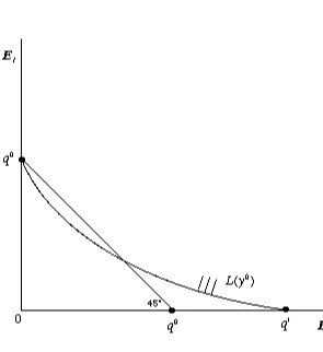
Figure 3 presents the set L(y0) that indicates feasible combinations of two energy inputs E₁ and

E2 to produce a given level of output y

0

. The boundary of the set is the traditional isoquant for

output y0. The point q0 on the _E1 axis indicates the minimum feasible quantity of input _E1

required to produce y0 when _E2 is not used. When instead q0 units of input _E2 are used instead

of _E1 it is no longer feasible to produce y0. Instead, to fully replace _E1 in production, q1 units of

E₂ are required. q0/_q1 _{is a measure of the total energy quality of E}

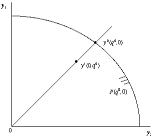
Figure 4 shows the feasible output set P(q0,0) for outputs y₁ and y₂ given input of q0 of _E1 and

zero of _E2.y0(q0,0) is one of the efficient output combinations that can be produced with these

levels of inputs. But for the input combination (0,q0) only a maximum of y1 can be produced

given the same output mix. The ratio of distances y1 /_y0 _{is a measure of the total energy quality}

of _E2 relative to _E1.

How does this measure relate to intrinsic qualities? Using the CES function in (12) the output

oriented total energy quality of _E2 relative to _E1 is given by:

y(0,q0) y(q0,0)=

"2 "1 #

$ % &

' ( 1

) *1 _A 2

A₁ (13)

which is the ratio of the augmentation factors multiplied by a constant which is a summary

statistic of the technology. The translog function cannot handle inputs with values of zero but for

a two input homogeneous generalized Leontief function the ratio of total energy quantities is:

y(0,q0) y(q0,0)=

"₂₂ "₁₁

A₂

A₁ (14)

The two concepts are, therefore, closely related. For more than two inputs or for

non-homogeneity such a simple relationship does not hold.

The indicators of energy quality discussed here would most likely be estimated using distance

functions estimated on cross-sectional data using either econometrics or more likely data

envelopment techniques.

Is the assumption that the interfuel elasticity of substitution is greater than one important? Stern

(2009) finds that at the level of the industrial sector the elasticity is only significantly greater

than unity for substitution between coal and gas and significantly less than unity for substitution

macro-economic level and more at the sub-industry level. However, these means based on the existing

empirical literature are likely to be biased downwards. The total substitution indicator of relative

energy quality may, therefore, be relevant, especially at the micro-level.

5. Fuel Quality: A Synthesis

We have seen that energy quality can be defined along the following dimensions:

Total vs. Marginal: Factor augmentation indices and distance-based indicators are measures of

total energy quality while relative prices are indicators of marginal energy quality.

Intrinsic vs. Substitution Based: Augmentation indices are measures of intrinsic energy quality

that do not depend on the quantities of other inputs or on how much energy is used and relate

well to the classical notion of use-value. They do, however, depend on the state of technology

unless some a priori assumption can be used to distinguish between changes in fuel quality and

technological change. In simple two input cases, the distance-based indicators are linear

functions of the ratios of the augmentation indices but in more general cases they depend on the

quantities of other inputs used and their augmentation indices. Relative marginal products are

usually a function of the quantities of inputs.

Absolute vs. Relative: An individual augmentation trend is an absolute indicator of energy

quality. All the other indicators are relative, though a single marginal product in real terms could

perhaps also be an absolute indicator. Relative augmentation trends net out the contribution of

factor neutral technical change and hence achieve a crude decomposition of changes in energy

quality and technological change.

But the existence and relevance of these various indicators also depend on the elasticity of

substitution between fuels. We can differentiate between the following cases:

Infinite Substitutability (σ = ∞): For the linear production function, marginal products are equal to augmentation indices. There is, therefore, a single indicator of absolute energy quality.

substitution-based measure of total energy quality is also equal to the ratio of marginal products

and the ratio of augmentation indices. Therefore, there is a single definition of relative energy

quality.

High Substitutability (∞ > σ > 1): All the measures of energy quality can be computed in theory, though in practice strong identifying assumptions are needed to identify augmentation

trends as quality factors. However, each indicator has a different value.

Cobb-Douglas (σ = _{1): Quality coefficients or augmentation indices cannot be identified.}

Low Substitutability (1 > σ > 0): The substitution-based indicator of total energy quality cannot be computed. Otherwise the indicators are similar to the high substitutability case.

Zero Substitutability ( σ = 0): We have not considered this case explicitly in the paper so far. The Leontief production function is given by:

y=min

[

]

where the γ’s are the minimum input requirements to produce one unit of output y. I few believe

that there is no reason for the technology to require varying amounts of energy from the different

fuels apart from differences in their quality, then the energy quality indices for each energy

input, E_{i, therefore are equal to} 1/_{"i. The function could be re-written in factor augmentation}

form as:

y=min

[

]

Therefore, only factor augmentation makes sense as an indicator of energy quality in this case

and neither of the substitution measures can be defined. On the other hand, if we believe that the

differences in the minimum input requirements are not entirely due to differences in quality we

As discussed in section 2, the quality coefficients can also:

• vary across fuels but do not depend on the use of fuels and do not vary over time.

• vary by fuel and use but do not vary change over time.

• vary by fuel (and possibly by use) and change over time possibly as a function of other

variables.

Marginal products might do any of the above, as will the total substitution measure. Neither is

defined based on restrictions in the way that quality coefficients are.

6. Aggregate Energy Quality

Using discrete Divisia aggregation:

"lnQ_t = 0.5

(

)

$

the change in the logarithm of the quality adjusted quantity index of energy Q, in period t, is the

sum of the cost share weighted changes in the logarithms of the quantities of the various fuels

E_{i. Dividing this index by the simple unweighted aggregate of fuels measured in heat}

equivalents (E) gives an index of aggregate energy quality. This approach is used almost

universally in the literature on quality adjustment of inputs.

Ho and Jorgenson (1999) define the quality of labor purely as the difference between the volume

index that takes into account substitution between different labor inputs (Equation 4 in their

paper) and the simple sum of labor hours. They are very explicit that one should not confuse

quality with factor augmentation, which is a particular parameterization of technological change.

Jorgenson and Griliches (1967, 257) go so far as to say that use of the term "quality change" for

this kind of adjustment for the effects of changes in the mix of inputs is a misnomer as all a

supposed increase in quality reflects is more rapid growth in the use of higher quality inputs than

lower quality inputs with no account taken of any change in the qualities of the individual inputs

improving over time, this change will be attributed to TFP while a shift from non-college

educated to college educated workers is attributed to quality change.

We can also develop an index of aggregate energy quality using the standard growth accounting

approach applied to (1). We take the total differential of the production function with respect to

time, divide both sides by y and multiply and divide each of the RHS variables by itself,

yielding:

d_lny dt =

"lny

"lnA d_lnA

dt +

"lny

"ln#i

d_ln#i

dt

i=1 n

$

"lnµ_i d_lnµ_i

dt

i=1 n

$

"lnE_i

d_lnE_i dt

i=1 n

$

"lnX_i d_lnX_i

dt

i=1 m

$

(18)

Now as each quality factor multiplies its factor of production the output elasticities with respect

to the quality factors are equal to those with respect to their inputs. In competitive equilibrium

under constant returns to scale the output elasticities are equal to the relevant cost shares and so

each of the latter four summations in (18) can be approximated in discrete form by a Divisia

index:

"lnZ

t = 0.5

(

)

$

where the Z’s are either energy inputs, other inputs, or quality factors. Of interest is an index of

energy quantity (20) and one of energy quality (21):

"lnQ_t = 0.5

(

)

i

$

"ln_#t= 0.5 S

it+Sit$1

(

)

i

%

Equation (20) is the standard index of aggregate energy input as proposed by Berndt (1978) and

of the inputs. If there are no such changes, then (20) is an appropriate method of aggregating the

energy inputs so that we can write:

y= f(A,"₁E₁,...,"_nE_n,µ₁X₁,...,µ_mX_m)=g(A,Q,µ₁X₁,...,µ_mX_m) (22)

If there are changes in the qualities, "i, but (21) is not actually computed then it will be absorbed

into the total factor productivity residual A.

It is clear, however, that the standard approach to computing a “quality-weighted” index in

equation (20) does not account for the effects of change in augmentation index style qualities.

While it might be weighted for differences in marginal products Q/E is not really an index of

energy quality from this perspective.

7. Conclusions

The arguments in this paper show that an index of energy volume/divided by aggregate heat

equivalent is not a complete indicator of aggregate energy quality. It may reflect the shift of the

energy mix towards higher or lower quality fuels but it will register no change when the relative

prices of any of the fuels in the mix changes but their quantity is unchanged. Also, I have

presented arguments to show why traditional demand curve use-value calculations cannot be

aggregated and are not informative regarding energy quality when an input is essential.

Several alternative indicators of energy quality are introduced. They are all equivalent only in the

case of linear production or infinite substitutability. I distinguished between measures of total

and marginal energy quality and between definitions of quality based on intrinsic properties of

each fuel (use-value) and based on substitution of one fuel for another (exchange-value).

Factor augmentation indices are an intrinsic total energy quality indicator. This indicator has

already been assumed to be the indicator of labor quality by Kazamaki-Ottersten et al. (1999)

and Mellander (2000) and is a development of the use-value indicators discussed in Stern (1999).

However, except in the cases of zero and infinite substitutability, measurement depends on

order to achieve any precision in estimation. There is also no obvious way to distinguish between

quality change and more general technological change.

I also introduced a new approach to measuring energy quality using distance functions. This is a

substitution based total energy quality indicator. The method can only be used if the elasticity of

substitution between energy inputs is greater than one. Relative prices are a straightforward

approach to measuring marginal quality from the substitution approach. They are useable for any

degree of substitutability between the energy inputs greater than zero. However, they only

collapse to the intrinsic quality indicator in the case of linear production.

Of course, there is nothing energy-specific about any of the arguments in this paper and the

proposed indicators can be applied to any other inputs too.

Acknowledgements

References

Abowd, J. M., Kramarz, F., Moreau A., 1996. Product quality and worker quality. Annales

d’Economie et de Statistique 41-42, 299-322.

Acemoglu, D., 2000. Labor- and Capital- Augmenting Technical Change. NBER Working Paper

7544.

Ayres, R. U., Warr, B., 2005. Accounting for growth: The role of physical work. Structural

Change and Economic Dynamics 16(2), 181-209

Berndt, E. R., 1978. Aggregate energy, efficiency, and productivity measurement. Annual

Review of Energy 3, 225-273.

Cleveland, C. J., Stern, D. I., 1993. Productive and exchange scarcity: an empirical analysis of

the U.S. forest products industry. Canadian Journal of Forest Research 23, 1537-1549.

Cleveland, C. J., Kaufmann, R. K., Stern, D. I., 2000. Aggregation and the role of energy in the

economy. Ecological Economics 32, 301-318.

Commons, J. R., 1934. Institutional Economics. New York, Macmillan.

Giannias, D. A., 1998. Labour quality and wage differentials. Scottish Journal of Political

Economy 45(2), 188-197.

Hanushek, E. A., Kimko, D. D., 2000. Schooling, labor-force quality, and the growth of nations.

American Economic Review 90(5), 1184-1208.

Harvey, A. C., 1989. Forecasting, Structural Time Series Models, and the Kalman Filter.

Cambridge, Cambridge University Press.

Harvey, A. C., Marshall, P., 1991. Inter-fuel substitution, technical change and the demand for

energy in the UK economy. Applied Economics 23, 1077-1086.

Hirschleifer, J., Hirschleifer, D., 1997. Price Theory and Applications. 6th edition, Prentice Hall,

Upper Saddle River NJ.

Ho, M. S., Jorgenson, D. W., 1999. The Quality of the U.S. Work Force, 1948-95. Kennedy

School of Government, Harvard University, Cambridge, MA.

Hunt, L. C., Lynk, E. L., 1993. The interpretation of coefficients in multiplicative-logarithmic

functions. Applied Economics 25, 735-738.

Jorgenson, D. W., Griliches, Z., 1967. The explanation of productivity change. Review of

Jorgenson, D. W., Ho, M. S., Stiroh, K. J., 2003. Lessons from the US growth resurgence.

Journal of Policy Modeling 25(5), 453-470.

Kander, A., 2002. Economic Growth, Energy Consumption and CO2 Emissions in Sweden

1800-2000. Lund Studies in Economic History, 19, University of Lund, Lund.

Kazamaki-Ottersten, E., Lindh, T., Mellander, E., 1999. Evaluating firm training, effects on

performance and labour demand. Applied Economics Letters 6, 431-437.

Mankiw, N. G., Romer, D., Weil, D. N., 1992. A contribution to the empirics of economic

growth. The Quarterly Journal of Economics 107, 407-437.

Mellander, E., 2000. The Multi-Dimensional Nature of Labor Demand and Skill-Biased

Technical Change. Research institute of industrial Economics, Stockholm, Sweden.

Padilla, S. B., Mayer, H. P., 2003. Sources of Growth in Selected Central and Eastern European

Countries. bP&Mayer Consultants, Ljubljana.

Pirsig, R. M., 1974. Zen and the Art of Motorcycle Maintenance. William Morrow.

Stern, D. I., 1999. Use value, exchange value, and resource scarcity. Energy Policy 27, 469-476.

Stern, D. I., 2009. Interfuel substitution: A meta-analysis. Munich Personal RePEc Archive

15792.

Tallman, E. W. and Wang, P., 1994. Human capital and endogenous growth: Evidence from

Taiwan. Journal of Monetary Economics 34, 101-124.

Turvey, R., Nobay, A. R., 1965. On measuring energy consumption. The Economic Journal 75,

Figure 1. Exchange- and Use-Value

Exchange Value Producer

Surplus

E* P *

Figure 2. Exergy Conversion Efficiencies, USA, 1900-1998