Convergence Analysis of General Version of Gauss Type Proximal Point Method for Metrically Regular Mappings

(1)

http://dx.doi.org/10.4236/am.2016.711110

Convergence Analysis of General Version

of Gauss-Type Proximal Point Method for

Metrically Regular Mappings

Md. Asraful Alom

1,2

, Mohammed Harunor Rashid

1

, Kalyan Kumer Dey

1

1_{Department of Mathematics, University of Rajshahi, Rajshahi, Bangladesh}

2_{Department of Mathematics, Faculty of Civil Engineering, Khulna University of Engineering & Technology,} Khulna, Bangladesh

Received 7 January 2016; accepted 17 July 2016; published 20 July 2016

This work is licensed under the Creative Commons Attribution International License (CC BY). http://creativecommons.org/licenses/by/4.0/

Abstract

We introduce and study in the present paper the general version of Gauss-type proximal point al-gorithm (in short GG-PPA) for solving the inclusion 0∈T x

( )

, where T is a set-valued mapping

which is not necessarily monotone acting from a Banach space X to a subset of a Banach space Y

with locally closed graph. The convergence of the GG-PPA is present here by choosing a sequence of functions g Xk: →Y with g 0k

( )

=0, which is Lipschitz continuous in a neighbourhood O of

the origin and when T is metrically regular. More precisely, semi-local and local convergence of

GG-PPA are analyzed. Moreover, we present a numerical example to validate the convergence re-sult of GG-PPA.

Keywords

Set-Valued Mappings, Metrically Regular Mappings, Lipschitz-Like Mapping, Local and Semi-Local Convergence

1. Introduction

We are concerned in this study with the problem of finding a point x∈ Ω ⊆X satisfying

( )

(2)

model for a wide variety of variational problems including complementary problems, system of nonlinear equations and variational inequalities. In particular, it may characterize optimality or equilibrium problems. Choose a sequence of functions g Xk: →Y with gk

( )

0 =0 which is Lipschitz continuous in a neighborhood O of the origin.

Martinet [1] proposed the following algorithm for the first time for applying it to convex optimization by considering a sequence of scalars

{ }

λk , which are different from zero:

(

1

)

(

1

)

0∈λk xk+ −xk +T xk+ , for each k=0,1, 2, (2) Rockafellar [2] thoroughly explored the method (2) in the general framework of maximal monotone inclusions. In particular, Rockafellar ([2], Theorem 1) shows that when xk+1 is an approximate solution of (2) and T is maximal monotone, then for a sequence of positive scalars λk the iteration (2) generates a sequence

{ }

xk which is weakly convergent to a solution of (1) for any starting point x0∈X. In [3], Aragón Artacho et al. have been presented the general version of the proximal point algorithm (GPPA) (see Algorithm 1), for the case of nonmonotone mappings, for solving the inclusion (1).

Let x X∈ . The subset of X, denoted by _{D x}k

( )

_{, is defined by}

( )

:

{

: 0

( )

(

)

}

.

k

D x = d X∈ ∈g d +T x d+ (3)

Thus we have the following algorithms which have been presented by Aragón Artacho et al. [3]:

Algorithm 1 (GPPA)

Step 1. Select x0∈X, λ∈(0,∞) and put k: 0= . Step 2. If 0 k( )

k D x

∈ , then stop; otherwise, go to Step 3.

Step 3. Put { } (λk ⊆ 0,λ), gk( )0 =0 and if 0∉D xk( )k , choose dk such that dk∈D xk( )k . Step 4. Set xk+1:=xk+dk.

Step 5. Replace k by k+1 and go to Step 2.

Note that, for a starting point near to a solution, the sequences generated by Algorithm 1 are not uniquely de-fined and not every sequence is convergent. The results obtained in [3] guarantee the existence of one sequence, which is convergent. Therefore, from the viewpoint of numerical computation, we can assume that these kinds of methods are not suitable in practical application. This drawback motivates us to introduce a method “so- called” general version of Gauss-type proximal point algorithm (GG-PPA). The difference between Algorithm 1 and our proposed Algorithm 2 is that the GG-PPA generates sequences, whose every sequence is convergent, but this does not happen for Algorithm 1. Thus we propose here the GG-PPA as follows:

Algorithm 2 (GG-PPA)

Step 1. Select η∈ ∞[ )1, , x0∈X, λ∈(0,∞) and put k: 0= . Step 2. If 0 k( )

k D x

∈ , then stop; otherwise, go to Step 3.

Step 3. Put { } (λk ⊆ 0,λ), gk( )0 =0 and if 0∉D xk( )k , choose dk such that dk∈D xk( )k and

( )

(

)

0, k .

k k

d ≤ηdist D x Step 4. Set xk+1:=xk+dk.

Step 5. Replace k by k+1 and go to Step 2.

We observe, from Algorithm 2, that

1) if g uk

( )

=λku and then we assume Y X= a Hilbert space, this algorithm reduces to the classical proximal point algorithm defined by (2).

(3)

A large number of authors have been studied on proximal point algorithm and have also found applications of this method to specific variational problems. Most of the study on this subject have been concentrated on vari-ous versions of the algorithm for solving inclusions involving monotone mappings, and specially, on monotone variational inequalities (see in [5]-[8]). Spingarn [9] has been studied first weaker form of monotonicity and for details see in [10].

There have a large study on local convergence analysis about Algorithm 1 (cf. [3][11][12]), but there is no semilocal analysis for Algorithm 1. A huge number of contributions have been studied on semilocal analysis for the Gauss-Newton method (cf. [4][13]-[16]). In [4], Rashid et al. have given a semilocal convergence analysis for the classical Gauss-type proximal point method. As our best knowledge, there is no study on semilocal anal-ysis for Algorithm 2. Therefore we conclude that the contributions presented in this study are seems new.

In the present paper, our aim is to study the semilocal convergence for the GG-PPA defined by Algorithm 2. The metric regularity property and Lipschitz-like property for set-valued mappings are mainly used in our study. The main results are convergence analysis, established in section 3, which based on the attraction region around the initial point and provide some sufficient conditions ensuring the convergence to a solution of any sequence generated by Algorithm 2. As a consequence, local convergence results for GG-PPA are obtained.

This paper is arranged as follows. In Section 2, some necessary notations, notions and preliminary results are presented. In Section 3, we consider the GG-PPA which is introduced in Section 1 and by using the concept of metric regularity property for the set valued mapping T, we will show the existence and present the convergence of the sequence generated by Algorithm 2. In Section 4, we present a numerical experiment to validate the se-milocal convergence of Algorithm 2. In the last Section, we will give a summary of the major results to close our paper.

2. Notations and Preliminary Results

In the whole paper, we assume that X and Y are Banach spaces. Let F be a set-valued mapping from X into the subsets of Y, denoted by _{F X}: _2Y_{. Let}_{x X}_∈ _and _r_>₀_{. The closed ball centered at}_x_{with radius}_r_is denoted by r

( )

x . The domain domF , the inverse F−1 and the graph gphF of F are respectively defined by

( )

{

}

dom :F = x X F x∈ : ≠ ∅ ,

( )

{

( )

}

1 _: _:

F− y ₌ x X y F x_∈ _∈

and

(

)

( )

{

}

gph :F = x y, ∈ ×X Y y F x: ∈ .

All the norms are denoted by ⋅ . Let A X⊆ and C X⊆ . The distance from x to A is defined by

(

)

{

}

dist ,x A : inf= x a a A− : ∈ for each x X∈ , while the excess from the set C to the set A is defined by

(

,

)

: sup dist ,

{

(

)

:

}

.

e C A = x A x C∈

From [4], we recall the following definition of metric regularity for set-valued mapping.

Definition 1 Let F X: Y be a set-valued mapping and let

(

x y,

)

∈gphF. Let rx >0,ry >0 and 0

κ

> . Then F is said to be

1) metrically regular at

(

x y,

)

on r_x

( )

x ×r_y

( )

y with constant κ if

( )

(

1

)

(

( )

)

( )

dist ,x F− y ≤κ dist ,y F x for all x∈r_x x y, ∈r_y y . (4) 2) metrically regular at

(

x y,

)

if there exist constants r_x′>0,r_y′>0 and

κ

>0 such that F is metrically regular at

(

x y,

)

on ′r_x

( )

x ×′r_y

( )

y with constant κ.

(4)

(

)

reg |F x y . The absence of metric regularity at x for y corresponds to reg |F x y

(

)

= ∞. The inequality (4) has direct use in providing an estimate for how far a point x is from being a solution to the generalized equation y F x∈

( )

and the expression dist ,

(

y F x

( )

)

measures the residual when y F x∈

( )

.

Recall the definition of Lipschitz-like continuity for set-valued mapping from [17]. This notion was intro-duced by Aubin in [18] and has been studied extensively.

Definition 2 Let _Γ:_Y_2X_{be a set}_-_{valued mapping and let}

(

_{y x}_,

)

_∈_gph_Γ_._Let _0, ₀

x y

r > r > and 0

M > . Then Γ is said to be Lipchitz-like at

(

y x,

)

on r_y

( )

y ×r_x

( )

x with constant M if the following

inequqlity hold:

( )

( ) ( )

(

1 rx , 2

)

1 2 for any , 1 2 ry

( )

.

e Γ y ∩_ x Γ y ≤M y −y y y ∈_ y (5) The following result establish the equivalence relation between metric regularity of a mapping F at

(

x y,

)

and the Lipschitz-like continuity of the inverse _F−1_at

(

_{y x}_,

)

_{, which is obtained from the idea in}_[19]_[20]_.

Lemma 1Let _{F X}: _2Y_{be a set valued mapping and} _{y F x}_∈

( )

_._Let _0, ₀

x y

r > r > , then F is metrically regular at

(

x y,

)

on r_x

( )

x ×r_y

( )

y if and only if its inverse F−1:Y 2X is Lipschitz-like at

(

y x,

)

on

( )

y x

r y × r x

  with constant

κ

>0 such that

( )

(

1 _, 1

)

_{for all ,}

( )

_.

x y

r r

e F− y _∩_ x F− y_′ _≤κ y y₋ _′ y y_′_∈_ y

We recall the following statement of Lyusternik-Graves theorem for metrically regular mapping from [21]. This theorem plays an important role in the theory of metric regularity and proves the stability of metric regularity of a generalized equation under perturbations. For its statement, we use that a set C X⊂ is locally closed at z C∈ if there exists a>0 such that the set C∩a

( )

z is closed.

Lemma 2 Consider a mapping _{F X}: _2Y_{and any}

(

_{x y}_,

)

_∈_gph_F_{at which}_gph_F_{is locally closed}_. Let F be metrically regular at x for y with constant

κ

>0. Consider also a function g X: →Y which is Lipschitz continuous at x with Lipschitz constant

λ

such that _{λ κ}_< −1_._{Then the mapping g F}₊ _{is metric}_- ally regular at x for y g x+

( )

with constant

1

κ κλ

− .

We finished this section with the following lemma, which is known as Banach fixed point theorem proved in [22].

Lemma 3Let _Φ:_X_2X_{be a set}_-_{valued mapping}_._Let

0 X

η ∈ , r∈

(

0,∞

)

and α ∈

( )

0,1 be such that

( )

(

0 0

)

(

)

dist η ,Φ η <r 1−α (6) and

( )

( ) ( )

(

1 r 0 , 2

)

1 2 for any ,1 2 r

( )

0 .

e Φ x ∩_ η Φ x ≤α x x− x x ∈_ η (7) Then Φ has a fixed point in r

( )

η0 , that is, there exists x∈r

( )

η0 such that x∈ Φ

( )

x . If Φ is additionally single-valued, then the fixed point of Φ in r

( )

η0 is unique.

3. Convergence Analysis of GG-PPA

In this section, we assume that _{T X}: _2Y_{is a set-valued mapping with locally closed graph at}

(

_{x y}_,

)

_∈_gph_T such that T is metrically regular at

(

x y,

)

with constant

κ

>0. Let :g X →Y be a (single-valued) function such that g

( )

0 =0, which is Lipschitz continuous in a neighborhood O of 0 with a Lipschitz constant

λ

>0. Let x X∈ and define a mapping Px by

( )

:

(

)

( )

. x

P ⋅ =g ⋅ −x T+ ⋅ (8) Then we obtain the following equivalence

( )

(

) ( )

1 _{for any} _and _.

x

z P y_∈ − _{⇔ ∈}y g z x T z_{− +} z X_∈ y Y_∈ ₍₉₎ In particular,

( )

(

)

1 _{for each ,} _{gph .} x

(5)

Let

(

x y,

)

∈gph

(

g T+

)

and let rx >0, 0ry > . Since g

(

⋅ −x

)

is Lipschitz continuous on O x+ , app-

lying the Lyusternik-Graves theorem (see Lemma 2) we assume that the mapping Px is metrically regular at

(

x y,

)

with constant

1

κ κλ

− , that is, by Lemma 1 we have the following inequality

( )

(

1 _, 1

)

_{for all ,}

( )

_.

1

x y

x r x r

e P− y _∩ x P− y_′ _≤ κ_κλ y y₋ _′ y y_′_∈ y

−

  (11)

Write

(

)

2 1 3

: min , .

2 4

y x x r r r

r λ κλ

κ

− −

 

= _ _

  (12)

Then

2 1

0 min , .

3 y x r r

r

λ

κ

 

> ⇔ < _ _

  (13)

The following lemma plays an important role for convergence analysis of the GG-PPA, which is due to [23].

Lemma 4Suppose that Px

( )

⋅ is metrically regular at

(

x y,

)

on rx

( )

x ×ry

( )

y with constant ₁

κ κλ

−

such that (12) and (13) are satisfied. Let

( )

2x

r

x∈ x and r_x

( )

0 ⊂O. Then Px−1

( )

⋅ is Lipschitz-like at

(

y x,

)

on

( )

2x

r y × r x

  with constant

1 3

κ κλ

− , that is,

( )

1 1

1 2 1 2 1 2

2

, for any , .

1 3

x

x r x r

e P y x P y κ y y y y y

κλ

− −

 

∩ ≤ − ∈

 

  ₋

   

For our convenience, we consider a sequence of functions g Xk: →Y with gk

( )

0 =0 which are Lipschitz continuous in a neighbourhood O of 0, the same for all k, with Lipschitz constants λk satisfying

1

: sup .

6 k k

λ λ

κ

= < (14)

We rewrite the mapping Px

( )

⋅ in (8) by substituting gk instead of g as follows:

( )

:

(

) ( )

for each 0,1,2, . k

x k

P ⋅ =g ⋅ − +x T ⋅ k= (15)

Since 1 1 6

λκ< < by (14), then by Lyusternik-Graves theorem (see Lemma 2) and Lemma 1 we obtain that

the mapping k 1

( )

x

P − _⋅ _{is Lipschitz-like at}

₍

_{y x}_,

₎

_on

_{( )}

y x

r y × r x

  with constant ₁ κ_κλ

− satisfying (11)

and hence we have

( )

{

: 0

(

)

}

.

k k

x

D x = d X∈ ∈P x d+ (16)

Furthermore, we define, for each x X∈ , the mapping Z Xx: Y by

( )

:

(

)

(

)

,

k

x k k

Z ⋅ =g ⋅ −x −g ⋅ −x (17) and the set-valued mapping k: 2X

x X

Φ  by

( )

_: 1

( )

_.

k k k

x Px− Zx 

Φ ⋅ = _ ⋅ _ (18)

(6)

( )

(

)

(

)

(

)

(

)

(

)

(

)

(

)

(

)

for each , .

k k

x x

k k k k

Z x Z x

g x x g x x g x x g x x

g x x g x x g x x g x x x x X

′ − ′′

′ ′ ′′ ′′

= − − − − − + −

′ ′′ ′ ′′ ′ ′′

≤ − − − + − − − ∈

(19)

The main result of this study given as follows, which provides some sufficient conditions ensuring the con-vergence of the GG-PPA with initial point x0.

Theorem 1 Suppose η>1 and that k

( )

x

P ⋅ is metrically regular at

(

x y,

)

on _r_x

( )

x ×_r_y

( )

y with

constant 1

κ κλ

− , and let r be defined in (12). Let rx

( )

x ⊂O and

δ

>0 be such that

a) min , , ,1,1

4 2 3 6

y

x r

r r λκ

δ

λ λ κλ

 − 

≤  

 ,

b)

(

η+3

)

κλ≤1, c) y <λδ. Suppose that

( )

(

)

lim dist , 0.

x x→ y T x = (20)

Then there exists some δ >ˆ 0 such that any sequence

{ }

xk generated by Algorithm 2 with initial point in

( )

ˆ x

δ

 converges to a solution _x*_{of (1), that is,} _x*_{satisfies that} ₀_∈_{T x}

( )

* _. Proof. Let

: .

1 3 t = ηκλ_κλ

− (21)

Then by assumption (b), (21) gives us

1.

t≤ (22) Assumption (c) and (20) allow us to take 0< ≤δ δˆ so that

( )

(

0

)

0 ˆ

( )

dist 0,T x ≤λδ for each x ∈δ x . (23) We will proceed by mathematical induction and show that Algorithm 2 generates at least one sequence and any sequence

{ }

xk generated by Algorithm 2 satisfies the following assertions

2 , k

x −x ≤ δ (24) and

1

1 k

k k x x t +

δ

+ − ≤ (25)

for each k=0,1, 2,. Define

(

5

)

(

)

: for each .

3 1

x

r κ y λ x x x X

λκ

= + − ∈

− (26)

Since η>1, by assumption (b) and (c), we have

( )

2

5 5 _{2 for each} _.

1 2

x

r ≤ ₋

κλ δ

_λκ

≤

_η

₊

δ

≤

δ

x∈δ x (27)

It is trivial that (24) is true for k=0. For showing that (25) is true for k=0, we need to prove that x1 exists, that is, 0

( )

0

D x ≠ ∅. We will prove 0

( )

0

D x ≠ ∅ by applying Lemma 3 to the mapping 0₀

x

Φ with x

(7)

( )

0 1 0 x x r

x P∈ − y ∩_ x by (10). Then by the mapping 0₀

x

Φ in (18) and the definition of excess e, we have

( )

(

)

(

( )

)

(

( )

)

( )

(

)

0 0 0 0

0

0 0 1 0 0 1 0

2

0 1 0 1 0

dist , , ,

,

x

x x r x x x

x r x x

x x e P y x x e P y x x

e P y x P Z x

δ

− −

Φ ≤ ∩ Φ ≤ ∩ Φ

 

≤ ∩ _ _

 

 (28)

(noting that

( )

0 2

x x

r x ≤ δ x ⊆ r x

   ). Now, by the choice of

λ

, we have

( )

(

)

(

)

(

)

(

)

0

0 0 0 0 0 0

0 0 0 .

x

Z x y g x x g x x y g x x g x x y

x x y x x y

λ λ

− = − − − − ≤ − − − +

≤ − + ≤ − + (29)

Since x0∈δˆ

( )

x ⊂δ

( )

x , by the fact 3λδ ≤ry in assumption (a) and y ≤λδ in assumption (c), for

each x∈δ

( )

x , (29) implies that

( )

0

0 ₂ _,

x y

Z x −y ≤ λδ ≤r (30) that is, for each x∈δ

( )

x , Zx0₀

( )

x ∈r_y

( )

y . In particular,

( )

(

)

( )

(

)

0

0 0 0 0 0

0 0 0

0

2 .

x

y

Z x y g x x y g g x x y

x x y x x y r

λ λ λδ

− = − − − ≤ − − +

≤ − + ≤ − + ≤ ≤ (31)

Hence by using (31) and Lemma 1 for Lipschitz-like property in (28), we have

( )

(

)

( )

(

)

(

)

0 0 0 0 0 0 dist , 1 1 2

1 1 .

5

x x

x

x x y Z x y x x

r r

κ κ _λ

κλ κλ

α

Φ ≤ − ≤ + −

− −

 

=_ − _ = −

 

This shows that assertion (6) of Lemma 3 is satisfied. Now, we show that the assertion (7) of Lemma 3 is satisfied. Let

( )

0

, r_x

x x′ ′′∈ x . Then by assumption (a) and (27), we have

( )

0 2

, r_x _rx

x x′ ′′∈ x ⊆δ x ⊆ x

and 0₀

( )

_, 0₀

( )

y

x x r

Z x Z′ x′′ ∈_ y by (30). By assumed Lipschitz-like property of 01

( )

x

P − ⋅ , we have

( )

(

)

(

( )

)

( )

(

)

( )

0 0 0 0 0

0 0

0 0 0 0

0 1 0 0 1 0

0 0 ( ), , , . 1 x x x

x r x x r x

x x r x x

x x

e x x x e x x x

e P Z x x P Z x

Z x Z x

κ κλ

− −

′ ′′ ′ ′′

Φ ∩ Φ ≤ Φ ∩ Φ

 ′   ′′ = _ _∩ _ _ ′ ′′ ≤ − −  

 (32)

Applying (19) in (32), we obtain

( )

(

)

(

)

(

)

(

)

(

)

(

)

0 0 0

0 0

0 0 0 0 0 0

0

,

1

2 2 _.

1 1

x

x r x

e x x x

g x x g x x g x x g x x

x x x x

κ κλ

κλ κλ

′ ′′

Φ ∩ Φ

′ ′′ ′ ′′ ≤ − − − + − − − − ′ ′′ ′ ′′ ≤ − ≤ − − −  (33)

Then by (14), (33) reduces to

( )

(

0 0 0

)

0 _, 0 2 2 _.

1 5

x

x r x

e x x x κλ x x x x α x x

κλ

′ ′′ ′ ′′ ′ ′′ ′ ′′

Φ ∩ Φ ≤ − ≤ − = −

−



This implies that the assertion (7) of Lemma 3 is also satisfied. Since both assertions (6) and (7) of Lemma 3 are fulfilled, we can deduce there exists a fixed point xˆ1∈rx₀

( )

x such that 0

( )

0

1 1

ˆ _x ˆ

x ∈ Φ x , which translates to

( )

0 0 0 1 1 ˆ ˆ x x

(8)

Now, we show that (25) is hold for k=0.

Note that r >0 by assumption (a). Then (13) is valid for (14). Since k 1

( )

x

P −

⋅ is Lipschitz-like at

(

y x,

)

on r_y

( )

y ×r_x

( )

x , it follows from Lemma 4 that the mapping

( )

1

k x

P − ⋅ is Lipschitz-like at

(

y x,

)

on

( )

2x

r y × r x

  with constant 1 3

κ κλ

− for each x∈r₂x

( )

x . In particular, 0

( )

1 0 x

P − ⋅ is Lipschitz-like at

(

y x,

)

on

( )

2x

r y × r x

  with constant 1 3

κ κλ

− as 0 ˆ

( )

2x

r

x ∈δ x ⊂δ x ⊂ x by assumption (a)

and the choice of δˆ. Furthermore, assumptions (a) and (c) imply that .

y <λδ ≤r (34) It seems that 0∈r

( )

y . Then by Lemma 1 we can say that the mapping 0

( )

0

x

P ⋅ is metrically regular on

( )

2x

r x

 relative to r

( )

y with constant _{1 3}

κ κλ

− . Thus by applying Lemma 1, we have

( )

(

₀₀ 1

)

(

₀₀

( )

)

0 0

dist , 0 dist 0,

1 3

x x

x P − ≤ κ_κλ P x

− (35)

and (23) implies that

( )

(

0

)

(

0

( )

)

(

( )

)

1

0 0

0 0 0

dist , 0 dist 0, dist 0, .

1 3 1 3 1 3

x x

x P − ≤ κ_κλ P x = λκ_κλ T x ≤ λκ δ_κλ

− − − (36)

Then from (16) and using (36), we obtain that

( )

(

₀

)

(

₀₀ 1

( )

)

0 0

dist 0, dist , 0 .

1 3

x

D x = x P − ≤ λκ δ_κλ

− (37)

From Algorithm 2 and using (21) and (37), we obtain that

( )

(

0

)

1 0 0 dist 0, 0 _{1 3} .

x x d η D x ηκλ δ tδ

κλ

− = ≤ ≤ <

− (38)

This implies that (25) is hold for k=0.

Suppose that the points x1, , xn have been obtained, and (24) and (25) are true for k=0,1, 2, , n−1. We will show that there exists a point xn+1 such that (24) and (25) also hold for k n= . Since (24) and (25) are true for each k n≤ −1, we have the following inequality

1 1

1 0

0 0 1 2 .

n n

i

n i

i i

t

x x d x x t

t

δ

δ δ δ δ

− −

+

= =

− ≤ + − ≤ + ≤ + ≤

−

∑

(39)

This reflects that (24) holds for k n= . Now with almost the same argument as we did for the case when 0

k= , we can find that the mapping n_n 1

( )

x

P − ⋅ is also Lipschitz-like at

(

y x,

)

on

( )

2x

r y × r x

  with constant

1 3

κ κλ

− . Then by applying again Algorithm 2, we have

( )

(

)

(

( )

)

( )

(

)

(

( )

)

(

)

(

)

( )

(

)

1 1

1 1 1 1 1

1 1

dist 0, dist , 0

dist 0, dist 0,

1 3 1 3

dist 0, 0

1 3 1 3

.

1 3 1 3 1 3

n

n n

n n n n n x

n

x n n

n n n n n n n

n n n

n n n n

x x d D x x P

P x T x

g x x g g x x

x x x x t t

η η

ηκ ηκ

κλ κλ

ηκ ηκ

κλ κλ

ηκλ ηκλ ηκλ _δ _δ

κλ κλ κλ

− + − − − − − + − − − − = ≤ = ≤ = − − = − − = − − − − ≤ − ≤ − ≤ ≤ − − − (40)

(9)

In the particular case, when x is a solution of (1), that is, y=0, Theorem 1 is reduced to the following corollary, which gives the local convergence of the sequence generated by the GG-PPA defined by Algorithm 2.

Corollary 1Suppose that η>1 and that x satisfies 0∈T x

( )

and that k

( )

x

P ⋅ is metrically regular at

( )

x,0 with constant

1

κ λκ

− . Let r>0 be such that 2r

( )

x ⊂O and suppose that

( )

(

)

lim dist 0, 0.

x x→ T x = (41)

Then there exists some δ >ˆ 0 such that any sequence

{ }

xk generated by Algorithm 2 with initial point in

( )

ˆ x

δ

 converges to a solution _x*_{of (1), that is,} _x*_{satisfies that} ₀_∈_{T x}

( )

* _. Proof. Since k

( )

x

P ⋅ is metrically regular at

( )

x,0 , there exist constants r0, rˆx and ₁₋κ_κλ such that

( )

k x

P ⋅ is metrically regular at

( )

x,0 on ˆr_x

( )

x ×r₀

( )

0 with constant ₁₋κ_κλ . Then, for each 0< ≤r rˆx, one has that

( )

(

1

)

(

( )

)

( )

₀

( )

dist , dist , for all , 0 .

1 x

k k

x x r r

x P − y ≤ κ_κλ y P x x∈ x y∈

−   (42)

Let supkλk:= ∈λ

( )

0,1 be such that

κλ

≤

_η

₊1₃. Choose rx∈

(

0,rˆx

)

such that r₂x ≤r and r0 rx₂ 0.

λ − >

Then

(

)

0 1 3

2

min , 0,

2 4

x x r r r

r = _ − λ −_κκλ _>

  (43)

and

0 1

min , , , 0.

4 2 3x 6

r r r λκ

λ λ κλ

−

 _{ >}

 

  (44)

Thus we can choose 0< ≤

δ

1 such that

0 1

min , , , .

4 2 3x 6

r r r λκ

δ

λ λ κλ

−

 

≤  

  (45)

Now it is routine to check that inequalities (a)-(c) of Theorem 1 are hold. Thus Theorem 1 is applicable to complete the proof of the corollary.

4. Numerical Experiment

We will provide, in this section, a numerical example to validate the semilocal convergence results of GG-PPA.

Example 1 Let X Y= =,x0=0.2,η=2,λ=0.2 andκ =0.5. Define a set-valued mapping T on by

( ) {

2 1,1

}

T x = − +x . Consider a sequence of Lipschitz continuous function gn with gn

( )

0 =0, which is

defined by

( )

1

3

n

g x = x. Then Algorithm 2 generates a sequence which is converges to _x*₌_0.5_.

It is obvious from the statement that T is metrically regular at

(

0.2,0.6

)

∈gphT and gn is Lipschitz continuous on the neighborhood of 0 with Lipschitz constant supkλk:= =λ 0.2. Consider T x

( )

: 2= − +x 1. Then from (3), we have that

( )

{

: 0

( )

(

)

}

3 6

: .

5 k

k k k k k k

k

k k

D x d g d T x d

x

d d

= ∈ ∈ + +

−

 

=_ ∈ = _

 



On the other hand, if k

( )

k

(10)

(

1

)

( )

1 1 3

0 .

5 k

k k k k k x

g x+ x T x+ x+ −

∈ − + ⇒ =

Thus from (40), we obtain that

1 . 1 3

k k

d ≤ ηκλ₋ _κλ d−

For the given values of , ,η λ κ, we see that _{1 3}ηκλ_κλ = <₇2 1

− . Thus, this implies that the sequence generated

by Algorithm 2 converges linearly. Then the following Table 1, obtained by using Mat lab program, indicates that the solution of the generalized equation is 0.5 when k=10.

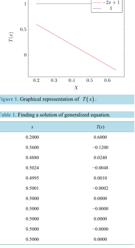
Moreover, in the case when T x

( ) {

= − +2x 1,1

}

, we can sketch the following Figure 1:

5. Conclusions

[image:10.595.212.422.307.471.2]

In this study, we have established semi-local and local convergence results for the general version of Gauss-type proximal point algorithm for solving generalized equation under the assumptions that η>1, a sequence of functions g Xk: →Y with gk

( )

0 =0 which is Lipschitz continuous in a neighbourhood O of the origin

[image:10.595.203.428.314.727.2]

Figure 1. Graphical representation of T x

( )

.

Table 1. Finding a solution of generalized equation.

x T(x)

0.2000 0.6000

0.5600 −0.1200

0.4880 0.0240

0.5024 −0.0048

0.4995 0.0010

0.5001 −0.0002

0.5000 0.0000

0.5000 −0.0000

0.5000 0.0000

0.5000 −0.0000

[image:10.595.200.427.514.720.2]

(11)

and T is metrically regular. Moreover, we have presented a numerical experiment to validate the semilocal convergence result for Algorithm 2. For the case where η=1, the question, whether the results are true for GG-PPA, is a little bit complicated. However, from the proof of the main theorem, one sees that all the results obtained in the present paper remain true provided that, for any x∈ Ω ⊆X, the following implication holds:

( )

such that min_{( )} .

d D x

D x ≠ ∅ ⇒ ∃ ∈d D x d = _∈ d

To see the detail proof of the above implication, one can refer to [17].

Acknowledgements

We thank the editor and the referees for their comments. Research of this work is funded by the Ministry of Science and Technology, Bangladesh, grant No. 39.009.002.01.00.053.2014-2015/EAS-19. This support is greatly appreciated.

References

[1] Martinet, B. (1970) Régularisation d’inéquations variationnelles par approximations successives. Revue Française D’automatique, Informatique, Recherche Opérationnelle, 3, 154-158.

[2] Rockafellar, R.T. (1976) Monotone Operators and the Proximal Point Algorithm. SIAM Journal on Control and Opti-mization, 14, 877-898. http://dx.doi.org/10.1137/0314056

[3] Aragón Artacho, F.J., Dontchev, A.L. and Geoffroy, M.H. (2007) Convergence of the Proximal Point Method for Me-trically Regular Mappings. ESAIM: Proceedings, 17, 1-8. http://dx.doi.org/10.1051/proc:071701

[4] Rashid, M.H., Wang, J.H. and Li., C. (2013) Convergence Analysis of Gauss-Type Proximal Point Method for Metri-cally Regular Mappings. Journal of Nonlinear and Convex Analysis, 14, 627-635.

[5] Auslender, A. and Teboulle, M. (2000) Lagrangian Duality and Related Multiplier Methods for Variational Inequality Problems. SIAM Journal on Optimization, 10, 1097-1115. http://dx.doi.org/10.1137/S1052623499352656

[6] Bauschke, H.H., Burke, J.V., Deutsch, F.R., Hundal, H.S. and Vanderwerff, J.D. (2005) A New Proximal Point Itera-tion that Converges Weakly But Not in Norm. Proceedings of the American Mathematical Society, 133, 1829-1835.

http://dx.doi.org/10.1090/S0002-9939-05-07719-1

[7] Anh, P.N., Muu, L.D., Nguyen, V.H. and Strodiot, J.J. (2005) Using the Banach Contraction Principle to Implement the Proximal Point Method for Multivalued Monotone Variational Inequalities. Journal of Optimization Theory and Applications, 124, 285-306. http://dx.doi.org/10.1007/s10957-004-0926-0

[8] Yang, Z. and He, B. (2005) A Relaxed Approximate Proximal Point Algorithm. Annals of Operations Research, 133, 119-125. http://dx.doi.org/10.1007/s10479-004-5027-9

[9] Spingarn, J.E. (1982) Submonotone Mappings and the Proximal Point Algorithm. Numerical Functional Analysis and Optimization, 4, 123-150. http://dx.doi.org/10.1080/01630568208816109

[10] Iusem, A.N., Pennanen, T. and Svaiter, B.F. (2003) Inexact Variants of the Proximal Point Algorithm without Monoto-nicity. SIAM Journal on Optimization, 13, 1080-1097. http://dx.doi.org/10.1137/S1052623401399587

[11] Aragón Artacho, F.J. and Geoffroy, M.H. (2007) Uniformity and Inexact Version of a Proximal Point Method for Me-trically Regular Mappings. Journal of Mathematical Analysis and Applications, 335, 168-183.

http://dx.doi.org/10.1016/j.jmaa.2007.01.050

[12] Pennanen, T. (2002) Local Convergence of the Proximal Point Algorithm and Multiplier Methods without Monotonic-ity. Mathematics of Operations Research, 27, 170-191. http://dx.doi.org/10.1287/moor.27.1.170.331

[13] Li, C. and Ng, K.F. (2007) Majorizing Functions and Convergence of the Gauss-Newton Method for Convex Compo-site Optimization. SIAM Journal on Optimization, 18, 613-642. http://dx.doi.org/10.1137/06065622X

[14] Li, C., Zhang, W.H. and Jin, X.Q. (2004) Convergence and Uniqueness Properties of Gauss-Newton’s Method. Com-puters & Mathematics with Applications, 47, 1057-1067. http://dx.doi.org/10.1016/S0898-1221(04)90086-7

[15] He, J.S., Wang, J.H. and Li, C. (2007) Newton’s Method for Underdetermined Systems of Equations under the Mod-ified γ-Condition. Numerical Functional Analysis and Optimization, 28, 663-679.

http://dx.doi.org/10.1080/01630560701348509

[16] Xu, X.B. and Li, C. (2008) Convergence Criterion of Newton’s Method for Singular Systems with Constant Rank De-rivatives. Journal of Mathematical Analysis and Applications, 345, 689-701.

(12)

[17] Rashid, M.H., Yu, S.H., Li, C. and Wu, S.Y. (2013) Convergence Analysis of the Gauss-Newton-Type Method for Lipschitz-Like Mappings. Journal of Optimization Theory and Applications, 158, 216-233.

http://dx.doi.org/10.1007/s10957-012-0206-3

[18] Aubin, J.P. and Frankowska, H. (1990) Set-Valued Analysis. Birkhäuser, Boston. [19] Rockafellar, R.T. and Wets, R.J-B. (1997) Variational Analysis. Springer-Verlag, Berlin.

[20] Ioffe, A.D. (2000) Metric Regularity and Subdifferential Calculus. Russian Mathematical Surveys, 55, 501-558.

http://dx.doi.org/10.1070/RM2000v055n03ABEH000292

[21] Dontchev, A.L., Lewis, A.S. and Rockafellar, R.T. (2002) The Radius of Metric Regularity. Transactions of the AMS, 355, 493-517. http://dx.doi.org/10.1090/S0002-9947-02-03088-X

[22] Dontchev, A.L. and Hager, W.W. (1994) An Inverse Mapping Theorem for Set-Valued Maps. Proceedings of the American Mathematical Society, 121, 481-498. http://dx.doi.org/10.1090/S0002-9939-1994-1215027-7

[23] Rashid, M.H. (2014) Convergence Analysis of Gauss-Type Proximal Point Method for Variational Inequalities. Open Science Journal of Mathematics and Application, 2, 5-14.