A
MODIFIED EKF ALGORITHM FOR GPS POINT DYNAMIC
POSITIONING AND VELOCITY MEASUREMENT
1, 2
SONG DAN, 1, 3 ZHANG PENGFEI, 1, 4 XU CHENGDONG
1
School of Aerospace Engineering, Beijing Institute of Technology, Beijing, 100081, China. E-mail: [email protected], 3 [email protected] ,[email protected]
ABSTRACT
Extended Kalman Filter (EKF) algorithm is widely used in GPS positioning and velocity measurement. As for EKF algorithm, the approximate initial position of the receiver is indispensable; otherwise the time consumption of the first positioning is too high because of the filter’s low convergence rate. A modified EKF algorithm named delayed update EKF (DU-EKF) algorithm for GPS point dynamic positioning and velocity measurement is proposed in this paper, which can speed up the convergence rate of the filter without the receiver’s approximate initial position. Furthermore, it can improve the accuracy of positioning and velocity measurement. Three kinds of algorithms are used in the simulation of this paper to compare with the modified EKF algorithm: iterative least square (ILS) algorithm, EKF algorithm with the Zero initial state vector (ZEKF) and EKF algorithm with the initial state vector which is Close to the actual situation (CEKF).
Keywords: Extended Kalman Filter (EKF), GPS, Positioning, Velocity measurement
1. INTRODUCTION
GPS point dynamic positioning and velocity measurement, with its excellence of only requiring a single frequency receiver, is widely used in vehicle navigation, marine positioning and field exploration for its low cost and high efficiency [1, 2]. Least Square (LS) algorithm [2] and Extended Kalman Filter (EKF) algorithm [3, 4] are commonly used for GPS point dynamic positioning and velocity measurement. As for LS algorithm, the approximate initial position of the receiver is indispensable because the pseudorange equation which depicts the range between the receiver and visible satellites should be linearized by Taylor series. To avoid searching for the approximate initial position and to achieve higher accuracy, modified algorithms based on LS have been proposed, such as weighted least square (WLS) algorithm [5] and iterative least square (ILS) algorithm [6]. Both of them can be used to position and measure velocity without the receiver’s approximate initial position, and thus higher accuracy can be obtained than that of LS algorithm. However, the accuracy is much lower than that of EKF algorithm [5, 7], just because LS algorithm only utilizes observation data belonging to the current epoch while EKF algorithm utilizes observation data of previous epochs as well [8]. As for EKF algorithm, the pseudorange equation and
the Doppler shift equation should also be linearized. Consequently, if the initial state vector deviates too much from the actual situation, convergence rate of filter will be very slow. In other words, it will take long time for the first positioning. Therefore, EKF algorithm also needs the approximate initial position of the receiver.
A modified EKF algorithm is proposed in this paper to position and measure velocity without the approximate initial position of the receiver, namely delayed update EKF (DU-EKF) algorithm in which the state error covariance matrix begins to be updated after several calculating epochs. This algorithm ensures a fast convergence rate and keeps the superior accuracy which EKF algorithm owns. To compare with the modified EKF algorithm, three kinds of algorithms are used in simulation of this paper. They are ILS algorithm, EKF algorithm with the Zero initial state vector (ZEKF) and EKF algorithm with the initial state vector which is Close to the actual situation (CEKF) respectively.
ISSN: 1992-8645 www.jatit.org E-ISSN: 1817-3195
motion. And Section 5 presents conclusions.
2. DESCRIPTION OF EKF ALGORITHM
FOR GPS POINT DYNAMIC POSITIONING AND VELOCITY MEASUREMENT
For GPS point dynamic positioning and velocity measurement, two kinds of models are used in EKF. One is the dynamic model describing the relationship of the receiver’s state vectors belonging to two adjacent epochs respectively, and the other is the observation model depicting the relationship between the observation vector and the receiver’s state vector. EKF requests to linearize the models which are nonlinear by Taylor series.
In terms of GPS point dynamic positioning and velocity measurement, the dynamic model can be CV model [10], CA model [11] or Singer model [9] which is linear while the observation model are both pseudorange model and Doppler shift model which are nonlinear. The basic EKF equations are as follows [9]:
State transition equation:
(1) Observation equation:
(2) State transition equation and observation equation correspond to dynamic model and observation model respectively. Formula (2) should be linearized to Formula (3):
(3) In Formula (1)-(3), k denotes epoch number; is the state vector at kth epoch, which incorporates all the receiver’s motion state
parameters needed to be solved; is the state transition matrix; is vector of dynamic model noise; is the noise driven matrix; is vector of observation noise; is the Jacobian matrix of
,namely observation matrix; ;
; .
The steps of EKF algorithm for GPS point positioning and velocity measurement are as follows ( and are covariance matrices of
and ):
1. Reckon the predictive state vector of : (4) Where is the optimal estimation of filteringfor .
2. Reckon which is the error covariance matrix of :
(5) 3. Calculate the Kalman gain matrix :
(6) 4. Get the optimal filtering estimation of :
(7) Where can be considered as the calculation result at kth epoch.
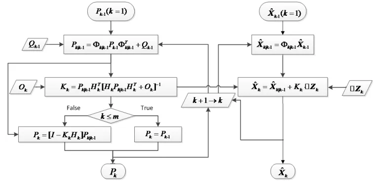
[image:2.612.119.491.530.703.2]5. Get the error covariance matrix of : (8) The process for EKF algorithm at kth epoch can be seen in Figure 1 [8].
3. DELAYED UPDATE EKF (DU-EKF) ALGORITHM FOR GPS POINT DYNAMIC POSITIONING AND VELOCITY MEASUREMENT
When using EKF algorithm for GPS point dynamic positioning, assigning to and a diagonal matrix with large positive elements to is an easy way of driving filter. However, as a result of the big difference between the zero vector and the actual , the slow convergence rate of filter elongates the time of first positioning [8]. Assigning a vector which is close to the actual to can accelerate the convergence rate of filter [3], nevertheless, it’s hard to define how close is to can make the filter converge fast. In addition, it is impossible to obtain the receiver’s approximate initial position all the time.
As seen in Figure 1, in EKF algorithm, the optimal filtering estimation of the state vector and its error covariance matrix are updated simultaneously at each epoch [1]. After a large number of experiments, one regulation is found which can accelerate convergence of filter and achieve higher accuracy. When using EKF algorithm for GPS positioning and velocity measurement, is still assigned to and its error covariance matrix to diagonal matrix with large positive elements. However, only is updated at each epoch, while begins to be updated after mth
epoch ( ). In other words, only is
updated when while and are both
updated when . Therefore a modified EKF algorithm, named DU-EKF algorithm, is proposed to utilize this regulation. The process of DU-EKF algorithm is shown in Figure 2, specific example of
is as follows:
At 1stepoch, input and , reckon , ,
and , , ;
At 2ndepoch, input and , reckon , ,
and , , ;
At 3rdepoch, input and , reckon , ,
and , , ;
At 4th epoch, input and , reckon , ,
and , , ;
(Same as at 4th epoch)
After a lot of experiments, it is found that: if , the convergence rate of filter can’t be improved. If , it takes only 5 epochs for the optimal estimation of filtering to approach the true value; from 10th epoch to 15th epoch, the precision of optimal filtering estimation can be the same as that of CEKF algorithm; after 15thepoch, the precision will be improved gradually and slightly. But if , the optimal estimation of filtering will not converge to the true value until a dozen of epochs. In other words, the convergence
rate of is much slower than that of
[image:3.612.114.497.516.702.2]. That’s why the range of m is from 2 to 6 in DU-EKF algorithm.
ISSN: 1992-8645 www.jatit.org E-ISSN: 1817-3195
4. SIMULATION
During the simulation of GPS point dynamic positioning and velocity measurement, pseudorange and Doppler shift are obtained from a simulator which produces pseudorange and Doppler data with Gauss white noise. The standard deviation of Gauss white noise for pseudorange and Doppler shift is 8m and 0.2m/s respectively. Moreover, the requirement of EKF algorithm that the initial conditions of the state of system and the priori statistical characteristics of error model should be zero mean white noise with known variances [1, 8] respectively is contented. Simultaneously, the simulation environment is close to the actual situation.
In the simulation, the receiver’s actual position is [5 ,5 , 0 ] m in geodetic coordinate system while
[6329853.79,553790.45,552184.40]m in Earth Centered Earth Fixed coordinate (ECEF) [12].The receiver is assumed to do uniform motion with a velocity of [5,5,5]m/s in ECEF. The initial simulation time is 2011-6-20 2:00:00 in UTC [13]. The simulation step is 1s, which means the interval between two adjacent epochs.
ILS algorithm, ZEKF algorithm and CEKF algorithm are all used to compare with DU-EKF algorithm. In ZEKF algorithm, CEKF algorithm
and DU-EKF algorithm, the Singer model [8] is chosen as the dynamic model and the quartz clock [7] is chosen as the clock model. The clock model is considered as the dynamic model of clock. Both the pseudorange and Doppler shift equations are chosen as observation model. The parameters of EKF based on these models are explained as follows:
1. Xk and Pk
[ , , , , , , , , , , ]
X u ux ux u uy uy u uz uz u u T
k= x vk k ak y vk k ak z vk k ak c t c fk k ˆ ˆ [ˆ ,ˆ ,ˆ ,ˆ ,ˆ ,ˆ ,ˆ ,ˆ ,ˆ , ˆ , ]
X u ux ux u uy uy u uz uz u u T
k= x vk k ak y vk k ak z vk k ak c t c fk k
| - | - | - | - | - | - | - | - | - |
-| - |
-ˆ [ˆ ,ˆ ,ˆ ,ˆ ,ˆ ,ˆ ,ˆ ,ˆ ,ˆ ,
ˆ
ˆ , ]
X u ux ux u uy uy u uz uz
k k 1 k k 1 k k 1 k k 1 k k 1 k k 1 k k 1 k k 1 k k 1 k k 1
u u T
k k 1 k k 1
x v a y v a z v a
c t c f =
Where [xuk,y zuk, uk], [ , , ]
ux uy uz
k k k
v v v , [akux,akuy,akuz] are the receiver’s position, velocity, acceleration in ECEF respectively; u
k t
and u
k f
are the receiver’s clock error and clock drift separately; Xˆ
k is the optimal estimation of filtering forXk; Xˆk k| -1 is the predictive state vector of Xk.
The error covariance matrix Pk of Xˆk is a matrix of 11 11× .
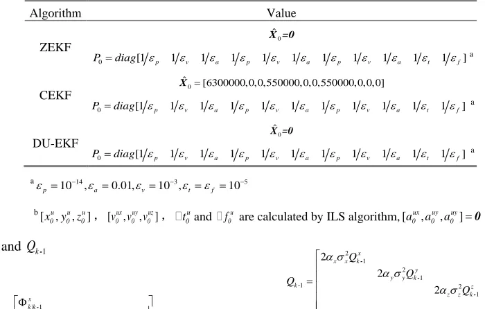
TheXˆ0and P0 for each algorithm can be shown
[image:4.612.125.475.464.687.2]in Table 1.
Table 1: The value of Xˆ0andP0for each algorithm
Algorithm Value
ZEKF
0 ˆ
X =0
0 [1 p 1 v 1 a 1 p 1 v 1 a 1 p 1 v 1 a 1 t 1 f]
P =diag ε ε ε ε ε ε ε ε ε ε ε a
CEKF 0
ˆ [6300000,0,0,550000,0,0,550000,0,0,0]
X =
0 [1 p 1 v 1 a 1 p 1 v 1 a 1 p 1 v 1 a 1 t 1 f]
P =diag ε ε ε ε ε ε ε ε ε ε ε a
DU-EKF
0 ˆ
X =0
0 [1 p 1 v 1 a 1 p 1 v 1 a 1 p 1 v 1 a 1 t 1 f]
P =diag ε ε ε ε ε ε ε ε ε ε ε a
a 14 3 5
10 , 0.01, 10 , 10
p a v t f
ε = − ε = ε = − ε =ε = −
b
[ u, u, u]
0 0 0
x y z ,[ux, uy, uz]
0 0 0
v v v , u
0
t
and u
0
f
are calculated by ILS algorithm, [ ux, uy, uy] 0 0 0 0
a a a =
2. Φk k| -1and Qk-1
| 1
| 1
| 1
| 1
| 1
-x
k k y k k
k k z
k k c k k
Φ
Φ
Φ =
Φ
Φ
2 1
2 1
-1 2
1
1
2
2
2
-x x x k
y y y k
k z
z z k c k Q
Q Q
Q Q α σ
α σ
α σ
=
Because the dynamic model is Singer model, | 1
k k
2
11 12 13
1 1 21 22 23
31 32 33
1
( 1 )
1
0 1 (1 )
0 0 | - -1 x x x T x x x x T
k k k
x T
T e
q q q
Q q q q
e
q q q
e α α α α α α − − − − + +
Φ = − =
-2 3 3 2 2 - 5
11
- -2 3
22 -2 33
(1- 2 2 3 - 2 - 4 ) 2
(4 - 3 - 2 ) 2
(1- 2 ) 2
x x
x x
x
T T
x x x x x
T T
x x
T x
q e T T T Te
q e e T
q e
α α
α α
α
α α α α α
α α
α
= + +
= +
=
-2 - - 2 2 4
12 21
-2 - 3
13 31
-2 - 2
23 32
( 1- 2 2 - 2 ) 2
(1- - 2 ) 2
(1 - 2 ) 2
x x x
x x
x x
T T T
x x x x
T T
x x
T T
x
q q e e Te T T
q q e Te
q q e e
α α α
α α
α α
α α α α
α α α = = + + + = = = = + y 1 k k
Φ | - and z 1 k k
Φ | - refer toΦx k|+1. -1
y k
Q and -1
z k Q refer to x-1
k
Q . αx ,αy ,αz are the reciprocal of the
maneuver time constant for each axis, 6
10
x y z
α =α =α = . 2
x
σ , 2
y
σ , 2
z
σ are the variance of the target acceleration in X,Y,Z respectively. T=1s,
2 2 2
100
= = =
x y z
σ σ σ [9].
The clock model [7] with white noise input comes from a second-order Markov process, as follows:
11 12
1 1 21 22
1
0 1
| -
-c c c c
k k k
c c
T q q
Q
q q
Φ = =
11 0 2 2 3
-1 -2 2 2 2 3 c h
q = T+ h T + π h T
12 21 2 3
-1 -2
2
c c
q =q = h T+π h T
22 0 2
-1 -2 8 2 2 3 c h
q h h T
T π
= + +
The parameters 20
0 9.4 10
h = × −
,
19-1 1.8 10
h = × −
,
21
-2 3.8 10
h = × − correspond to values for a typical quartz standard.
3. Hk and Ok
k
H is linearized from 1 1
(X =) n n T
k k k k k k
f R R D D . Where s
k
R and s k
D is respectively the pseudorange Formula (9) and the Doppler shift Formula (10) [1] between a visible satellite and the receiver,
1, ,
s= n (n is the total number of visible satellites).
2 2 2
( ) ( ) ( )
s s u s u s u u
k k k k k k k k
R = X −x + Y −x + Z −z + ⋅c t
(9)
[( ) ( ) ( ) ( )
( ) ( )]
s u sx ux s u sy uy
k k k k k k k k
s u sz uz
s k k k k u
k s k
k
X x V v Y y V v
Z z V v
D c f
ρ
− ⋅ − + − ⋅ − + − ⋅ −
= + ⋅ (10)
In Formula (9) and Formula (10), [ k, k, k]
s s s
X Y Z and
[ sx, sy, sy]
k k k
V V V are position and velocity vector of the sth visible satellite in ECEF, s
k
ρ is the actual range between the sth visible satellite and the receiver,
2 2 2
= ( ) ( ) ( )
s s u s u s u
k Xk xk Yk yk Zk zk
ρ − + − + − .
| | |
| | |
| | | | | |
| | | | | |
1 1 1
1x k 1 y k 1z k
1 1 1
nx k ny k nz k
k 2 1 2 1 2 1
1x k 1x k 1 y k 1 y k 1 y k 1z k
2 1 2 1 2 1
nx k nx k ny k ny k nz k nz k
h 0 h 0 h 0 1 0
h 0 h 0 h 0 1 0
H
h h h h h h 0 1
h h h h h h 0 1
=
Elements from Line 1 to Line n of Hk is
linearized from Formula (9) while from Line n+1 to Line 2n of Hk is linearized from Formula (10).
| -|
| -ˆ
( u s)
s s
k k 1 k
1 k k
sx k u ux s
k k k k 1
x X
R D
h
x v ρ
− ∂ ∂ = = = ∂ ∂ | - | - | - | -| | -ˆ ˆ ( )( ) ( ) ( )
ux sx s 2 u s s
s
k k 1 k k k 1 k k 1 k k k 1
2 k
sx k u s 2
k k k 1
v V x X J
D h x ρ ρ − − − ∂ = = ∂
2 2 2
| -1 ( ˆ| -1) ( ˆ| -1) ( ˆ| -1)
s s u s u s u
k k Xk xk k Yk yk k Zk zk k
ρ = − + − + −
| -1 | -1 | -1 | -1
| -1 | -1
ˆ ˆ ˆ ˆ
( ) ( ) ( ) ( )
ˆ ˆ
( ) ( )
s s u sx ux s u sy uy
k k k k k k k k k k k k k
s u sz uz
k k k k k k
J X x V v Y y V v
Z z V v
= − ⋅ − + − ⋅ −
+ − ⋅ −
where |
1 sy k
h and |
1 sz k
h refer to 1 sx k
h | ; |
2 sy k
h and 2
sz k
h | refer to 2
sx k
h | .
The covariance matrixOk of the observation
noise vector is a matrix of 2n×2n,
[
1 1 2 2]
=
k
O diag o o o o ,o1=64,o2=0.04.
4. Zk and Zk
1 1
Z = n n T
k rk rk dk dk
| - | - ˆ| - ˆ|
-ˆ ˆ
[ , , ,( ), ,( )]
Z 1 1 n n 1 1 n n
k= rk −rk k 1 rk −rk k 1 dk−dk k 1 dk −dk k 1
( ) ( ) ;
2 2 2
| -1 1 1 1
1
ˆ ( ˆ ) ( ˆ ) ( ˆ )
ˆ
s s u s u s u
k k k k k k k k k k k
u k k
r X x Y x Z z
c t = − + − + − + ⋅ | - | - | | - ;
| -1 | -1 | -1 | -1
| -1 | -1
| -1 | -1
| -1
ˆ ˆ ˆ ˆ
[( ) ( ) ( ) ( )
ˆ
( ) ( )]
ˆ ˆ
s u sx ux s u sy uy
k k k k k k k k k k k k s u sz uz
k k k k k k
s u
k k s k k
k k
X x V v Y y V v
Z z V v
d c f
ρ
− ⋅ − + − ⋅ −
+ − ⋅ −
= + ⋅
Where s k
r and s k
d are the pseudorange and the Doppler shift of sth visible satellite respectively.
ISSN: 1992-8645 www.jatit.org E-ISSN: 1817-3195
shown in Figure 2.
With respect to the result of each algorithm, the position and velocity error of X, Y and Z are respectively shown in Table 2 and Table 3.
Table 2: Position error of each axis for different algorithms (m)
Axis Algorithm Mean value Standard
deviation
Root mean square
X
ILS -0.3041 8.9346 8.9397
CEKF 0.0213 1.4897 1.4898
DU-EKF -0.0269 1.3784 1.3786
Y
ILS 0.4654 5.0010 5.0226
CEKF -0.0427 0.8759 0.8769
DU-EKF -0.1841 0.7081 0.7316
Z
ILS -0.0109 3.9734 3.9734
CEKF -0.4672 0.5392 0.7135
DU-EKF -0.0913 0.4778 0.4864
Table 3: Velocity error of each error for different algorithms (m/s)
Axis Algorithm Mean value Standard deviation
Root mean square
X
ILS -0.0038 0.0407 0.0409
CEKF -0.0071 0.0154 0.0170
DU-EKF 0.0038 0.0129 0.0134
Y
ILS 0.0006 0.0259 0.0259
CEKF 0.0031 0.0077 0.0083
DU-EKF -0.0012 0.0084 0.0084
Z
ILS -0.0018 0.0184 0.0185
CEKF -0.0051 0.0073 0.0089
DU-EKF -0.0011 0.0070 0.0071
5 55 105 155 205 255 305
- 10 - 5 0 5 10
Epoch
P
os
i
t
ion
er
ror
/
m
Posi t i on er r or of Z
DU- EKF CEKF I LS
Figure 3: The position error of Z for different algorithms
5 55 105 155 205 255 305
- 0. 06 - 0. 04 - 0. 02 0 0. 02 0. 04 0. 06
Epoch
V
el
o
c
ity
e
r
ro
r
/m
/s
Vel oci t y er r or of Z
DU- EKF CEKF I LS
Figure 4: The velocity error of Z for diffeent algorithms
Figure 3 and Figure 4 are the position error figure and velocity error figure of Z respectively. At the beginning 20 minutes of simulation for ZEKF algorithm, the position and velocity errors are much larger than other algorithms. So they are only shown in Figure 5. As shown in Figure 3 and Figure 4, combining the statistic data in Table 2 and Table 3, the position and velocity error of ILS algorithm are within 10m and 0.05m/s respectively; the position and velocity error of CEKF algorithm are within 2m and 0.02m/s respectively; the position error of DU-EKF algorithm are within 1.5m while the velocity error are within 0.02m/s. Compared with ILS algorithm, the precision of position and velocity of DU-EKF algorithm are much higher. Compared with CEKF algorithm, the precision of position and velocity of DU-EKF algorithm is not improved appreciably. But DU-EKF algorithm can accelerate the filter’s convergence rate without the approximate value of the initial state vector.
0 200 400 600 800 1000 1200
-500 0 500 1000 1500 2000
Epoch
P
o
sitio
n
e
rr
o
r/m
a. P ositon error of Z
DU-EKF ZEKF
0 200 400 600 800 1000 1200
-10 -8 -6 -4 -2 0 2
Epoch
V
elo
c
ity
e
rr
o
r/
m
/s
b. Velocity error of Z
DU-EKF ZEKF
As shown in Figure 5, when Xˆ0 is far from the actualX0, the slow convergence of filter impedes
dynamic positioning with extending the time of first
positioning. Figure 5 demonstrates the
effectiveness of DU-EKF algorithm in accelerating convergence rate of filter.
5. CONCLUSION
The example of uniform motion receiver is used in simulation of this study. By simulation, compared with ILS algorithm, CEKF algorithm and ZEKF algorithm, the effectiveness of the modified algorithm for EKF (DU-EKF algorithm) is demonstrated in GPS point dynamic positioning and velocity measurement. The results of DU-EKF algorithm have much higher precision than that of ILS algorithm and slightly higher accuracy than that of CEKF algorithm. DU-EKF algorithm solves the problem of low filter convergence rate without the initial approximate initial position of receiver (compared with ZEKF algorithm). DU-EKF algorithm sets the initial state vector as 0which is far from the true value. However with the delayed updating of state error covariance matrix, the optimal estimation of filtering can be close to the actual state vector quickly.
If DU-EKF algorithm is used in actual GPS navigator, there is no need of receiver’s initial approximate initial position all the time when it changes in a wide range. Meanwhile, higher precision of positioning and velocity measurement and less time consumption of first positioning can be reached. However, whether the DU-EKF algorithm can be applied in other areas or not should be further validated.
ACKNOWLEDGMENTS:
This work was supported by the National High-Tech. R&D Program, China (No.2011AA120505) and the National Natural Science Foundation, China (No.61173077).
REFRENCES:
[1] Bernhard Hofmann-Wellenhof et al, “GNSS global navigation satellite systems GPS, GLONASS, Galileo & more”, Springer-Verlag, New York, 2008.
[2] Qing Chang et al, “GPS positioning algorithm based on least-square recurrence estimate”, Journal of Beijing University of Aeronautics and Astronautics, Vol. 24, No. 3, 1998, pp. 263-266.
[3] Fred Daum, “Nonlinear filters: beyond the Kalman filter”, IEEE A&E SYSTEMS MAGAZINE, Vol. 20, No. 8, 2005, pp. 57-69. [4] Juang JC, Huang GS, “Application of Kalman
filter and mean field annealing algorithms in GPS-based attitude determination”, Journal of navigation, Vol. 51, No. 1, 1998, pp. 117-131. [5] Gangyi Tu et al, “Implementation and validity
of three GPS positioning optimization algorithms”, Journal of Chinese inertial technology, Vol. 17, No. 2, 2009, pp. 170-174. [6] Tong HB et al, “Iterative reweighted recursive least squares for robust positioning”, Electronics letters, Vol. 48, No. 13, 2012, pp. 789-791.
[7] Xuchu Mao et al, “Nonlinear iterative algorithm for GPS positioning with bias model”, IEEE intelligent transportation systems conference, October 3-6, 2004, pp. 684-689.
[8] Chui CK, Chen G, “Kalman filtering with real-time applications”, 2nd ed, Springer-Verlag, New York, 1991.
[9] Robert A. Singer, “Estimating optimal tracking filter performance for manned maneuvering targets”, IEEE Transaction on aerospace and electronic systems, Vol. AES-6, No. 4, 1970, pp. 473-483.
[10] Hampton RLT, James R. Cooke,
“Unsupervised tracking of maneuvering Vehicle”, IEEE Transaction aerospace and electronic systems, Vol. AES-9, No. 2, 1973, pp. 197-207.
[11] Moose RL, Vanlandingham HF, McCabe D.H., “Modeling and estimation for tracking maneuvering targets”, IEEE Transaction aerospace and electronic systems, Vol. AES-15,No. 3, 1979,pp. 448-456.
[12] Pengfei Zhang et al. “Coordinate transformations in satellite navigation systems. Advances in electronic engineering, communication and management”, lecture notes in electrical engineering, Vol. 140, 2012, pp. 249-257.
[13] Pengfei Zhang et al. “Time scales and time transformations among satellite navigation systems”, China satellite navigation conference (CSNC) 2012 proceedings, lecture notes in Electrical Engineering, Vol. 160, Part 3, 2012, pp. 491-502.
[14] Qiuying Guo, Zhenqi Hu, “Several algorithms for GPS pseudorange absolute positioning”, Science of surveying and mapping, Vol.