SENTIMENT ANALYSIS USING REPRESENTATIVE TERMS A GROUPING APPROACH FOR BINARY CLASSIFICATION OF DOCUMENTS

(1)

ISSN: 1992-8645 www.jatit.org E-ISSN: 1817-3195

FAULT DIAGNOSIS FOR MOTOR BASED ON EMD

ALGORITHM

LIJUN WANG, DONGFEI WANG, YONGLIANG HUANG

School of Mechanical Engineering, North China University of Water Resources and Electric Power,

Zhengzhou 450011, Henan, China

ABSTRACT

Nowadays motor is the most widely used power supply equipment and drive. In order to ensure the reliable operation of the motor, it is necessary to analyze the fault mechanism of motor equipment and to do some research on the relevant technology about fault diagnosis. The motor diagnostic method based on signal processing is the way that relies on modern signal processing technology to extract fault features, and find the fault according to the characteristics. At present the fault diagnosis method based on the wavelet analysis has become a hot topic. But wavelet transform also has its own defects, such as its dependence on a priori information and its applicable limitation. However, Empirical Mode Decomposition (EMD) as a new signal processing technology, is completely driven by its original signal, doesn't need a priori base function and overcomes the deficiency of the wavelet transform. Therefore in this paper, EMD method is used in the fault diagnosis of the motor. In this study, EMD method shows a great advantage in the aspects of signal feature extraction, transformation, the reduction feasibility and fault diagnosis for induction motor at a setting speed.

Keywords: Empirical Mode Decomposition, Fault Diagnosis, Signal Processing, Feature Extraction

1. INTRODUCTION

It is accepted that the motor is the most widely used power supply equipment and drive nowadays. With regard to the production of electric energy, almost all the electrical energy is produced by generators. And in terms of the consumption of electrical energy, more than 70% of the electricity is consumed or converted into other energy by motor in the world. In addition, the motor has become ubiquitous in people's daily life and is inseparable from any industry sector for many pieces of equipment are driven by motors. While complex operating environment and diffident load property make a higher failure rate possible in their running process especially when they are operated in some bad operation conditions and with great

impact load. Therefore，it is necessary to analyze

the fault mechanism of motor equipment and to do some research on the relevant technology about fault diagnosis of the motor.

In recent 40 years, motor fault diagnosis technology has developed rapidly, produced huge economic benefits and become a hot issue studied in various countries. Many authoritative institutions were involved in this area, such as the United States mechanical engineering society (ASME) and NASA. Many universities and companies also set up a diagnosis technology research centers. Guo

qing An, Jiao min Liu et al[1] propose the

correlation fundamental component filtering

method to diagnose rotor broken bar fault in motor; Ying Shao[2] put forward a new method based on the rotating Park transformation filtering to monitor the rotor complicated condition of induction motor.

Compared with wavelet analysis method, Hilbert-Huang transform (HHT) put forward by an American engineer named Norde. E.Huang in 1998 is a new signal analysis method. HHT theory consists of Empirical Mode Decomposition (EMD) and Hilbert transformation. The basic idea of this theory is that: firstly decompose the original signal into a series of Intrinsic Mode Functions (IMF) by EMD; secondly do Hilbert transformation for each IMF; and then derivate the phase of the data after doing Hilbert transformation; at last find out the

meaningful instantaneous frequency and

instantaneous amplitude of each IMF and obtain Hilbert spectrum of the original signal.

(2)

reflect the frequency information of the original signal, and accurately diagnose the fault type of motors.

2. THE PRINCIPLE OF EMPIRICAL MODE

DECOMPOSITION

Hilbert-Huang Transformation (HHT) theory is composed of empirical Mode decomposition and

Hilbert transformation，and contains two basic

concepts: One is instantaneous frequency; the other is Intrinsic Mode Function (IMF). Some concerned concepts of HHT theory are introduced in follows.

2.1.The Instantaneous Frequency

The traditional concept of frequency is defined as the number of vibrations finished in one second, which reflects the overall features of the signal in a period of time. This definition is correct for smooth and stable signals, while for those non-stationary signals, the traditional definition of frequency is not accurate, because the frequency of non-stationary signal changes with time. Therefore, instantaneous frequency is introduced. Given a time series, Hilbert transformation is defined as follows:

1 ( )

( ) X t

H t P d

t τ

π τ

+∞

−∞ =

−

∫

(1)

Where P is Cauchy principal value, generally P= 1;

Such a real signal x t and ( ) H t can form a ( )

complex signalZ t : ( )

( )

( ) ( ) ( ) ( ) j t

Z t =X t +jH t =a t eφ (2) Where

2 2

( ) ( ) ( )

a t = X t +H t , ( ) arctan ( )

( ) H t t

X t

φ =  

  (3)

From the formula 1, it can be seen that Hilbert transformation of the signal is convolution of the signal itself and reciprocal of time. It reflects the partial feature of the signal. According to the type 2, the instantaneous frequency is defined as follows:

( )

( )t d t

dt

φ

ω = (4)

Or ( ) 1 ( )

2

d t

f t

dt

φ π

= (5)

By type 4, it can be seen that instantaneous frequency not only is the function of virtual signal, but also is a function of time. This is the accepted definition of instantaneous frequency, but there are several contradictions in this definition. Firstly instantaneous frequency might not belong to the original signal; secondly instantaneous frequency

may be negative frequency with no significance; thirdly the instantaneous frequency of band limited signal may be beyond band range [3].

2.2.Intrinsic Mode Function（（（（IMF））））

The concept of intrinsic modal function is put forward by Doc. Huang on the basis of summarizing previous studies, aiming to make

instantaneous frequency meaningful. If the

instantaneous frequency of a IMF is meaningful in any point, it must meet the following two conditions: firstly the number of extreme points and the number of zero points must be equal or different

from 1 in all data；Secondly in any data point, the

maximum value envelope and the minimum mean envelope of the signal local all are zero. Namely the curve of signal is locally symmetric about time axis. The former demand is similar to narrowband requirement of steady-state gauss signal, while the latter one changes global requirements into local requirements to prevent the volatility of the instantaneous frequency [4].

The decomposition process of EMD can be considered as a "screening" process, in which the original signal is decomposed into sum of each IMF arranged one by one from high frequency to low frequency[5].Steps of decomposition process are shown as follows:

Step one: At first, find out all the maximum and minimum points of the signal to deal with, and then use cubic spline interpolation to deal with these extreme value points respectively; at last, work out the up envelope line and low envelope line of the signal, and Figure out the mean of the envelopes. In Figure 1, curve a stands for the original signal, curve b is for maximum envelope and curve c is for minimum envelope.

Step two: take the value of x t ( )

subtracting m t( ) notes for h t₁( ) ,

namelyh t₁( )=x t( )−m t( ) and then check whether

1( )

h t meets two demands of IMF or not. If not,

make h t as the signal to deal with and repeat the ₁( )

above step until h t accords with two demands of ₁( )

IMF, noting r ( )₁ t =x t( )−h t₁( ) . Next Figure out

( )

x t subtractingc t , noting₁( ) r ( )₁ t =x t( )−h t₁( ).

Step three: make r ( )₁ t as a new signal and repeat

[image:2.612.143.259.596.647.2]

(3)

Figure 1: Extreme envelope

So the original signal x t can be expressed as ( ) the sum of several IMFs and remainder term.

1

( ) ( ) ( )

n

i n

i

x t c t r t

=

∑

+ (6)

It should be noted that Step three will not stop until one of the following conditions is met: the last

remainder item c tn( ) become smaller than the

expected value; the remainder item c t_n( ) is a

monotone function. Theoretically, if the number of decomposition is not restricted, such decomposition will last forever. To make the decomposed IMF be of actual physical significance, it is necessary to limit the number of decomposition. Norden E.Huang [6] has given a Cauchy convergence

criteria, namely the standard deviation value SD of

1( )

k

h− t and h tk( ).

2 1

2

0 1

( ) ( )

( ) T

k k

t k

h t h t

SD

h t ε

−

= −

 ₋ 

=  〈

 

 

∑

(7)

When the standard deviation value SD is less

than the set value, the decomposition process will

stop. Norden E.Huang suggested SD take one value

between 0.2 and 0.3. It is necessary to write control algorithm to apply EMD to signal processing in the computer. The process of decomposition EMD flow chart is shown in Figure 2.

start

input signalx t( )

1, ( )n ( ) n= r t =x t

is monotone functions or less than expected value?

( )

n

r t

0( ) n( ), 1

h t =r t i=

get local maximum value and minimum value

1( )

i

h− t

calculate the upper envelope and lower envelope

1( )

e t

2( )

e t

1 2 1

( ) ( ) ( )

2

i

e t e t

m− t = +

1 1 ( ) ( ) ( )

i i i

h t =h− t−m− t

is IMF ?h ti( )

end 1

( ) ( ), ( ) ( ) ( ), 1

n i n n n

c t =h t r+ t =r t −c t n= +n N

Y

N

[image:3.612.268.521.58.486.2]

1 i= +i Y

Figure 2: The Flow Chart For EMD Decomposition

2.3.Hilbert Marginal Spectrum

The original signal can be expressed as

1

( ) ( ) ( )

n

i n

i

x t c t r t

=

∑

+ (8)

Making useful IMF Hilbert transformed and ignoring remainder item, type8 can approximately expressed as:

(

)

( ) Re ( ) exp ( )

1 n

x t a t_i j _i t dt

i ω

= ∑ ∫

= (9)

It can be seen that type 9 is a function for

tandω. IfH( , )ω t =x t( ), it can be got:

1

( , ) Re ( ) exp( ( ) )

n

i i

H ω t a t j ω_i t dt

=

(4)

This is Hilbert spectrum. From type 10, it can be seen that Hilbert spectrum reflects rules of the signal amplitude changing with frequency and time in the whole frequency band.

According to type 10, marginal spectrum can be defined:

0

( ) ( , )

T

h w =

∫

H ω t dt (11)

Hereh w( ) is called Hilbert marginal spectrum,

in which T stands for the length of sampling time. From the type 11, it can be seen that Hilbert marginal spectrum of the signal describes the rule of amplitude changing with the frequency and represents the stack of amplitudes in a certain frequency place in the whole time period. Therefore, Hilbert marginal spectrum breaks the limitation of traditional Fourier spectral, not only preventing revealing each frequency components, but also of very high resolution ratio [7].

3. THE APPLICATION OF EMD IN PRACTICE

In order to explain how to apply EMD to practice, an example is taken. It is supposed that the original

signal x t( )=sin(2πt+10) cos(5+ πt+1) and

sampling frequency is 100 Hz. The decomposition process of EMD is shown in Figure 3.

[image:4.612.317.516.180.505.2]

Analyzing the decomposition of the results, it can be seen that IMF1 and IMF2 are got after the original signal is processed by EMD and the IMFs are arranged from high frequency to low frequency. This also shows that EMD can be used in filtering. In order to prove that the sum of decomposition signal is consistent with the original signal, the sum of IMF1 and IMF2 is figured out. The result is shown in Figure 4.

Figure 3: EMD Decomposition Examples

From Figure 4, it can be seen, the sum of IMF1 and IMF2 is the same as the original signal basically. Through the method of spectrum analysis, several steps have been taken: decomposing the

original signal, and then doing Hilbert

[image:4.612.319.519.181.322.2]

transformation for each IMF, finally figuring out Hilbert marginal spectrum as shown in Figure 5.

Figure 4: The Sum Of IMF1 And IMF2 Compared With The Original Signal

Figure 5: The Signal Marginal Spectrum

It can be seen the main spectrum is 1 Hz and 2.5 Hz, which is consistent with the original signal from Figure 5. So it can be concluded that EMD method can truly restore the frequency information of the original signal, and it can be used to extract the original signal characteristics.

4. THE APPLICATION OF EMD IN MOTOR

FAULT DIAGNOSIS

[image:4.612.94.293.551.686.2]

(5)

assembly conditions, such as broken rotor bars, uneven air gap and inter turn short circuit between the stator. When it happens to fail, the type of the motor fault may be single one or a combination of several faults. Generally speaking, there are two methods to study the motor fault: one way is that diagnose faults by collecting parameters of the current when the motor runs. It is because that the current flowing through the coil will change when motors have failures; the other way is that diagnose faults by collecting the vibration data when the motor runs. It is because that the vibration will be in abnormalities when the motor is in fault.

In this paper, the second way is chose to diagnose the motor faults. So the below works should been done: installing vibration sensors in the motor, setting the sampling frequency as 1000Hz and the sampling points as 1024, before starting to diagnose faults.

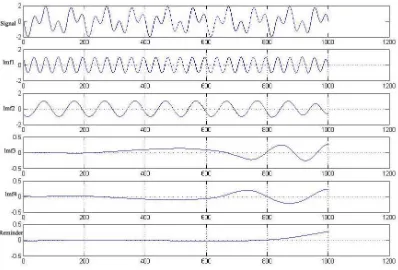
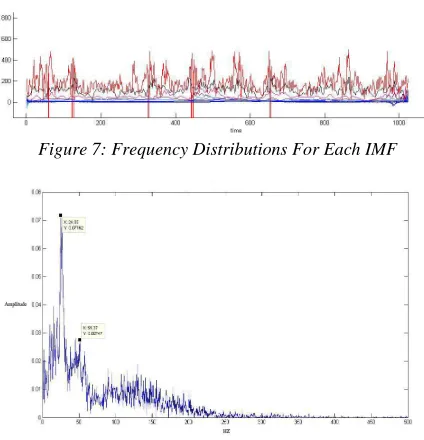
First of all, process the original signal using EMD method, and the result is shown in Figure 6. From this picture, it can be seen that the original signal is broken down into nine IMFs, of which the top five’s amplitude are the larger than the rest’s, and whose characteristics are similar with characteristics of the original signal. Secondly do Hilbert transformation to the nine IMFs. The frequency distribution maps of each IMF after transforming are shown in Figure 7. From this figure, it can be seen that nine curves change with time and the nine curves correspond to the instantaneous frequency of the nine IMF at different times. It can be concluded that EMD method is able to obtain the instantaneous frequency of the signal. At last, Figure out the marginal spectrum of these nine IMFs as shown in Figure 8.

[image:5.612.314.526.99.319.2]

Figure 6: The EMD Decomposition Figure For Vibration Data

Figure 7: Frequency Distributions For Each IMF

Figure 8: The Original Signal’s Marginal Spectrum

When the motor speed is 1480RPM, it can be known that the rotation frequency of the motor is 24.7Hz. From Figure 8, it can be seen that there is 24.95Hz frequency components next to 24.7Hz. So it can be assumed that 24.95Hz frequency is the motor rotation frequency. It is because that there is not often a peak in the theory rotational frequency, due to the frequency accuracy of the frequency spectrum analysis. At the same time, if there is

significant frequency component in the range (± ∆f)

of theory rotation frequency, it can be considered that the component is the rotational frequency. It can be also seen that there is large amplitude frequency component in one frequency doubling. Meanwhile, there is a large amplitude frequency (51.37Hz) in twice frequency doubling. According to the characteristic frequency table as shown in table 1, it can be preliminarily judged that there are rotor imbalance fault and rotor misalignment fault in the motor. However, due to the small amplitude in this two frequency, (only 0.07mm / s and 0.03mm / s), it can be determined that the vibration of the motor is not severe.

Table 1: Part Of The Characteristic Frequency For Motor’s Vibration

Fault type Characteristic frequency

Rotor imbalance 1×RPM Rotor misalignment 1×RPM，2×RPM Clearance vibration 0.4~0.5×RPM，1~5×RPM

Bearing loose Various times frequency and fractional frequency Short circuit of Stator

laminated, phase resistance imbalance, etc

(6)

Generally speaking, the amplitudes of the motor spectrum in one frequency doubling and twice frequency doubling are larger than other frequency

amplitudes，but the absolute amplitude is small.

Therefore, according to the characteristic frequency table, the motor have potential faults of rotor imbalance and rotor misalignment. Especially, the possibility of rotor imbalance fault happening is higher than the probability of rotor misalignment fault.

5. CONCLUSION

In this study two aspects of work are completed as follows: Firstly, with the application of EMD method, we process a stable periodical original signal with procedures of decomposition, feature extraction, and spectrum analysis, and the results of these processes are in accordance with the spectrum of the original signal. It proves that the EMD method can restore the frequency information of the original signal. At the same time, it is feasible to extract the characteristic of original signal with the application of EMD method. Secondly, faults of asynchronous motor with a speed of 1480 RPM are diagnosed based on EMD method in this paper. With the motor signals gathering with the application of vibrating sensor of which the sampling frequency is 1000HZ, and procedures of decomposition, the acquirement of marginal spectrum, the analysis of marginal spectrum for acquired signals. At last, it can be concluded that the motor rotor have the potential failure of imbalance and misalignment of rotary through comparing with the frequency characteristics table of vibration control motor, and especially the failure probability of rotor imbalance is higher than the misalignment of rotary.

ACKNOWLEDGEMENT

This project was supported by National Nature Science Foundation of China (51076046), and also was supported by Key Plan Projects of Science and

Technology of Henan province in

China(102102210034) and Startup Research

Foundation for High Level Talents of North China University of Water Resources and Electric Power.

REFERENCES:

[1] Guoqing An, Jiaomin Liu, Liwei Guo, Yukun

Liu, “Diagnosing rotor broken bar fault in motor by using correlation fundamental

component filtering method”, Electric

Machines and Control, Vol. 15, No.3, 2011, pp. 69-73.

[2] Ying Shao, “Feature extracting method of

stator and rotor faults of induction motor by park vector rotating filter”, Electric Machines and Control, Vol. 14, No. 3, 2010, pp. 57-61.

[3] Johansson. The Hilbert Transform, Master

Thesis, Vaxjo University, Vaxjo, Sweden, 1999.

[4] Lijun Wang， Yongliang Huang， Dong fei

Wang, “Abnormal combustion fault diagnosis of hydrogen-fueled engine based on EMD”, Journal of Harbin Institute of Technology, Vol. 18, No. 12, 2011, pp. 90-92.

[5] M L Wu, S Schubert, Norden E.Huang，“The

development of the South Asian summer monsoon and the intrapersonal oscillation”, Journal of Climate, Vol. 12, No. 11, 1999, pp. 2054-2075.

[6] N. EH. “A new method for nonlinear and

non-stationary time series analysis: Empirical 4mode decomposition and Hilbert spectral analysis”, Proc of SPIE, Vol. 4056, No. 16, 2000, pp. 197-209.

[7] P.D. Spanos, A. Giaralis, N.P. Politis,

“Time-frequency representation of earthquake

accelerograms and inelastic structural response

records using the adaptive chirplet

decomposition and empirical mode