http://dx.doi.org/10.4236/ojfd.2015.52019
A Kinematics Scalar Projection Method
(KSP) for Incompressible Flows with
Variable Density
Jean-Paul Caltagirone
1, Stéphane Vincent
21UMR CNRS 5295, Département TREFLE, Institut de Mécanique et d’Ingénierie, Université de Bordeaux, Pessac Cedex, France
2UMR CNRS 8208, Laboratoire Modélisation et Simulation Multi Echelle (MSME), Université Paris-Est, Marne-La-Vallée, France
Email: [email protected], [email protected]
Received 13 April 2015; accepted 12 June 2015; published 15 June 2015
Copyright © 2015 by authors and Scientific Research Publishing Inc.
This work is licensed under the Creative Commons Attribution International License (CC BY). http://creativecommons.org/licenses/by/4.0/
Abstract
A new scalar projection method presented for simulating incompressible flows with variable den-sity is proposed. It reverses conventional projection algorithm by computing first the irrotational component of the velocity and then the pressure. The first phase of the projection is purely kine-matics. The predicted velocity field is subjected to a discrete Hodge-Helmholtz decomposition. The second phase of upgrade of pressure from the density uses Stokes’ theorem to explicitly compute the pressure. If all or part of the boundary conditions is then fixed on the divergence free physical field, the system required to be solved for the scalar potential of velocity becomes a Poisson equa-tion with constant coefficients fitted with Dirichlet condiequa-tions.
Keywords
Projection Methods, Hodge-Helmholtz Decomposition, Navier-Stokes Equation, Incompressible Flows
1. Introduction
resolu-tion of the equaresolu-tion of moresolu-tion for the applicaresolu-tion of the incompressibility constraint together with the formula-tion of an equaformula-tion for pressure [3]. One important aspect is immediately apparent to the first authors who have developed numerical algorithms around finite volume methods, i.e., the spatial location of pressure and velocity unknowns. For collocated variables, instabilities appear and interpolations are needed to mitigate and remove these fluctuations of velocity and pressure [4]. Harlow and Welch in 1965 had introduced the notion of stag-gered variables [5] initially for two-phase flows. This strategy, called the Marker and Cell Method, ensures the coupling, direct or not, of the pressure and velocity fields without disturbance.
Since many authors have developed time splitting or prediction-correction methods called projection that in-volve treating the solving of motion equations and their incompressibility constraint sequentially. Many algo-rithms allow obtaining convergence orders in time ranging from range O
( )
∆t1/ 2 to O( )
∆t2 . These orders also depend on the boundary conditions imposed. Some reviews can be found on these techniques including the comprehensive of Guermond et al. [6]. The more recent use of these techniques for the simulation of two-phase flows leads to ill-conditioned linear systems especially for strong density contrasts. Indeed solving a Poisson equation with strongly varying coefficients is very costly in terms of number of iterations of iterative solvers such as conjugate gradient. The direct solvers are efficient in two-dimensional space but are unusable in three- dimensional simulations for large numbers of degrees of freedom. Some authors address the problem on an al-gebraic point of view by specific preconditioning or by the resolution of a saddle point [7]-[10]. Other ways are sought for example by Guermond et al. [11] [12] extracting the density of the Poisson equation. This approach is effective mainly for small density ratios. It can be used with some caution for flows involving open boundary conditions [13]. The recent fast pressure-correction method of Dodd and Ferrante [14] is also based on the fac-torization of the density in the projection step by using of the minimum density between two separated fluids with the introduction of a pressure source term in the Poisson equation. This method has been validated against standard capillary test cases and it was utilized to simulate the interaction between a homogeneous isotropic turbulence and 6260 spherical particles. Works based on a vector approach of the resolution of the projection step [15] [16] are particularly effective for the simulation of two-phase flows with large density contrasts. How-ever, it requires the solving of large linear systems induced by the coupling of all velocity components in the projection. In the same field, parallel works centered on the discrete Helmholtz-Hodge decomposition bring po-tential solutions to use it for solving partial differential equations such as Navier-Stokes equations [17] [18]. Other potential applications of this decomposition are numerous. They are detailed in the review of Bhatia et al. [19].The approach proposed here is based entirely on the mechanics of discrete media [20]. This formulation of the momentum conservation equation results in a set of equations that is different from the standard Navier-Stokes equations. Its constitution resumes from the fundamental law of dynamics, Newton’s second law, and on a vi-sion of differential geometry. Thus a discrete equation of motion is obtained in the form of a natural decomposi-tion of Helmholtz-Hodge in irrotadecomposi-tional and solenoidal parts. This approach has led to a purely vectorial version of the projection method where at the end of this second step the boundary conditions of the problem are satis-fied [21]. The present work is devoted to a scalar version of vectorial projection where irrotational components of the velocity are sought by a Helmholtz-Hodge decomposition of the scalar potential of velocity. A detailed presentation of the projection algorithm is first given and several illustrative examples of flows with varying densities are provided for discussion.
2. Kinematics Scalar Projection (KSP) Method
The resolution of the equation of motion in an incompressible formulation associated with the boundary condi-tions of the physical problem is the objective of projection methodologies. These motion equacondi-tions can be the Navier-Stokes equations or the equations coming from the discrete mechanics [20]. For flows at constant density and at constant viscosity, both formulations are equivalent whereas it is not the case for variable fluid properties encountered in two-phase flows for example. As this choice is regardless for the scalar projection method under consideration here, the Navier-Stokes equations of motion for an incompressible flow are resumed
(
)
d d
0
t
p t
ρ µ
= −∇ + ∇ ⋅ ∇ + ∇
∇⋅ =
V
V V
V
where V is the velocity, t the time, p the pressure, ρ the density and μ the dynamic viscosity. The boundary of the physical domain Ω is noted Σ. By decomposing the material derivative of velocity and discretizing equations at first order in time (a second order is easily obtained with the present method by using a second order Taylor expansion in time), a prediction step can be formulated for the intermediate velocity V*:
(
)
n
n * n t
n 1
p t
ρ ρ µ
+ ΨΣ
− + ⋅∇ = −∇ + ∇ ⋅ ∇ + ∇
∆
× = ×
*
* *
*
V V
V V V V
V n V n
(2)
with pn the pressure at time n t∆ , ∆t the time step and VΨΣ the solenoidal component of the desired ve-locity on the boundary
Σ
, that is Vn+1 for a time discretization for which tn+1 represents the time at the end of the prediction and projection steps of the time splitting approach. Two-phase flows with variable density en-compass a wide variety of different physical situations. For example, a liquid-particle gas flow does not present the same difficulties as a hydraulic jump flow even if the density ratio is the same. In the second case, this is the difference in density associated with the gravity that generates the flow motions. In many cases, the algorithms described in the introduction section are sufficient to simulate the physical behavior of the problem. The Helm-holtz-Hodge decomposition of the predicted velocity field is sufficient to maintain the balance between the ef-fects of gravity and the dynamic efef-fects even if the field VΦ is not exactly an irrotational field. This is the case for example for the natural convection presented in Section 3.2. In the absence of the incompressibility con-straint in the equation of motion in the prediction step, the divergence of V* is not zero and only the normal velocity component is respected at the boundaries. The predicted field V* =VΦ+VΨ includes both solenoidal and irrotational contributions. The divergence free component V* is known on Σ thanks to the physical boun-dary condition to impose. However, the projection step does not allow maintaining it as it is related to a scalar equation. The scalar projection step consists in searching the irrotational component VΦ = ∇Φ and then obtain the divergence free component by difference with V*. One of the Helmholtz-Hodge decomposition methods of the velocity V*= ∇Φ + ∇×Ψ into its two divergence and rotational free components amounts to applying the divergence operator to V* and ∇Φ that are equal since the divergence of the rotational is zero. It can be demonstrated [6] that null flux conditions on the scalar potential have to be associated to the Poisson equation2
0 on
∇ Φ = ∇ ⋅
∇Φ ⋅ = Σ
* V
n
(3)
for Dirichlet boundary conditions on V*. Other types of boundary conditions can be also considered as dis-cussed for example in [6] [13] [22]. In fact it can be built as many irrotational fields as boundary conditions ap-plied to the system. However, there is little chance of finding a solenoidal field that satisfies the boundary condi-tions of the physical problem. This step is purely kinematics and does not result from any numerical time split-ting. It does not involve either the density which is perfectly legitimate. The flow may be a variable density or two-phase immiscible flow, there is no physical reason or mathematical argument that leads to associate the density in the scalar potential velocity Φ. The dynamic part of the projection step contrariwise brings up the density for the pressure p. The following of the section specifically returns to the link between the scalar poten-tial of velocity and pressure.
The first equation of system (2) is a prediction step. It can be solved with the physical boundary conditions of the problem. Its solution V* does not satisfy the divergence free constraint. Indeed, the solving of this predic-tion step with a scalar potential pn not adapted to the boundary conditions of incompressibility and unknown at the solving time of the prediction step introduces a non-zero irrotational component that has to be removed by means of Helmholtz-Hodge decomposition. The second equation of (1) cannot be solved directly as the actual component VΦ of the actual field has to be deduced from the difference between the fields V* and VΨn 1+
obtained after the decomposition of the field V*. It can be observed that VΦ =VΦn+1 derives from a potential
Φ= ∇Φ
1 1 , . n n n n n p t p t ρ ρ + + − = −∇ ∆ − = −∇ ∆ * V V V V (4)
By subtraction of these two equations, we obtain:
(
1)
.
n 1 *
n n
p p
t
ρ + − = −∇ + −
∆
V V
(5) We also have
(
)
(
)
0* n 1
n 1 * *
+
Φ Ψ Φ
+
Φ Ψ
= ∇Φ + ∇ × = + = +
∇ ⋅ = ∇ ⋅ − = ∇ ⋅ − ∇Φ = ∇ ⋅ = ∇ ⋅∇ × =
V V V V V
V V V V V
Ψ
Ψ (6)
By combining (5) and (6), an equation linking the pressure increment p′ =pn+1−pn and the irrotational
ve-locity component can be written:
.
p t
ρ
Φ = ∇ ′∆
V
(7) By using (3) and (7), we finally get the KSP projection step
2 p t ρ Φ Φ
∇ Φ = ∇⋅ = ∇Φ ∇ =′ ∆ * V V V (8)
The pressure increment is obtained by considering the Stokes theorem
d .
b
b a
a
l
∇Φ ⋅ = Φ − Φ
∫
t (9)According to (8) and (9),
d d .
b b
b a
a a
p p p l l
t
ρ
Φ
′− ′ = ∇ ⋅′ = ⋅
∆
∫
t∫
V t (10)Equation (10) is correct only if
t
ρ Φ
∆
V
is a gradient. On a discrete point of view, ρ is constant over each mesh
edge and Δt is also constant, so that
t t t
ρ ρ Φ =ρ∇Φ= ∇ Φ
∆ ∆ ∆
V
is clearly a gradient and expression (10) always holds, even for multi-phase flows, as soon as a fluid-fluid interface is part of mesh edges as in unstructured or ALE approaches. Finally, the update of the velocity and pressure fields is given by expressions:
1 1
d
n 1 n 1
b
n n
b a
a
p p l
t ρ + + Ψ Φ + + Φ = = − ′ = ′ + ⋅ ∆
∫
*V V V V
V t (11)
where a and b correspond to vertices, endpoints of the edges Γ forming the computational mesh where the den-sity is constant. This last relation corresponds to the application of one of the forms of the Stokes theorem which allows updating the potential geometrically if the velocity field is irrotational, which is the case. In the particular situation where the segment Γ is intersected at point c by an interface separating fluids of densities ρ1 and ρ2, i.e.
1 1 1 d 2 d
c b
n n
b a
a c
p p l l
t t
ρ ρ
+ +
Φ Φ
′ = ′ + ⋅ + ⋅
∆ ∆
∫
V t∫
V t (12)As for the velocity, it stays continuous and constant along all the segment. Point c will be determined thanks to an interface tracking method of VOF, Front-Tracking or Level-Set type [23] [24].
The pressure at time n + 1 is then pn+1= pn+p′. Practically, we start integrating the pressure increment from an arbitrary mesh point for which ρ is known (belonging to one phase or another) and by stating p′ =0 at this point. This procedure is valid on structured or unstructured grids. The algorithm finally obtained is very simple to implement:
• Prediction step: solving of the first equation of system (2) to obtain V*.
• Projection step: decomposition of the field V* in a gradient of the potential Φ and a rotational part by using system (3).
• Estimate of the irrotational component VΦ= ∇Φ and of the solenoidal component by using the difference
1
.
n+
Ψ = *− Φ
V V V
• Update of the velocity and pressure by considering (11)-(12).
The solution at the next time step tn+1 consists of the pressure and divergence free velocity. It does not meet the imposed tangential physical boundary conditions as do the other projection methods. A boundary layer is so created that disappears during the time iterations with the imposition of the physical boundary conditions in the two stages of prediction and correction. The thermodynamic pressure p is in fact utilized only to evaluate the properties of the fluids such as the density and the viscosity. For multi-phase flows at constant densities, the Bernoulli pressure is well adapted in this case. The present KSP algorithm, also called DSP by [21] in the frame- work of discrete mechanics equations, inverts the calculation steps for pressure and velocity compared to stan-dard projection approaches. For classical projections methods, the pressure is first estimated as the solution of a Poisson equation with variable coefficients and the velocity is then explicitly obtained. In the KSP method, the velocity is first decomposed by a purely kinematics process and the pressure is then updated by the explicit ap-plication of the Stokes theorem. The solving of a Poisson equation with variable coefficients is a difficult task whose complexity increases with density ratios, especially with large grids on massively parallel computers, whereas the KSP method is not sensible to these density variations.
When high density gradients are associated to large magnitude source terms, it can be necessary to perform a preliminary Helmholtz-Hodge decomposition of source terms s acting in the momentum equations, before the time evolution loop begins. In this way, the initial condition for pressure at mechanical equilibrium is then built as
0 0 0.
s
p Φ p
−∇ +s = −∇ + ∇Φ = (13)
The initial condition is given by p0= Φs. The source term s=sΦ+sΨ= ∇Φ + ∇×s Ψs. The contribution
s
Ψ = ∇×
s Ψ does not directly induce a pressure. However, it generates the motion through the increase of the solenoidal velocity field. As a consequence, sΨ has to be kept in the momentum equations instead of s when the treatment of pressure initial condition (13) is implemented. On the contrary, a source term deduced from a gradient field does not involve any flow motion. In this configuration, it is directly integrated inside the pressure gradient to form a new pressure field. The decomposition of the initial source term s is achieved by using a Poisson equation similar to (3) so as to obtain Φs:
2
0 on s
s ∇ Φ = ∇ ⋅
∇Φ ⋅ = Σ
s
n (14)
Prior decomposition of the source term eliminates the adverse effects induced by exchanges between the pressure effects and all the other effects (viscous, inertial) that cause unwanted local and instant acceleration that affects the quality of the two-phase behavior. This KSP version suitable for very constrained two-phase flows,
vector field by the scalar potential that it contains whereas the latter do not participate to the movement itself.
3. Illustration Test Cases
3.1. Static Equilibrium between Two Fluids under Gravity Effects
The considered problem is very simple, it consists of a square cavity of unit height filled with two immiscible fluids whose densities are ρ1 and ρ2. It is assumed that the two fluids are initially separated and the heavy fluid 1 occupies the lower half of the cavity. The stationary solution is simple: the velocity V is zero and the pressure field satisfies p y
( )
= p0+ρ( )
y g e⋅ yy. The initial pressure field is zero. The walls of the cavity are assumed impermeable and adherent, VΨ=0.Details of the different steps of the time splitting algorithm on this problem are the following. In the absence of initial velocity, the velocity field derived from the prediction step (2) is V e⋅ y = −∆ t g. If this field is
diver-gence free within the cavity, this is not the case near horizontal walls due to boundary conditions. Assuming in-compressibility, these variations of divergence restore a linear distribution of the scalar potential of the velocity along the vertical axis. The numerical solution of Φ obtained up to a constant by solving the Poisson Equation (3) is represented by its evolution along y as
t g y
Φ = −∆ (15) The irrotational velocity field is VΦ⋅ey = ∇Φ ⋅ey= −∆tg. The difference V*−VΦ =0 is the requested ve-locity such that n+1 0
Ψ Φ
= = *− =
V V V V . The pressure update by the Stokes theorem is then
( )
1 0 n
[image:6.595.220.406.492.674.2]p + =p −
ρ
y gy (16) where p0 is the reference pressure chosen in an arbitrary manner. At the end of the two stages the theoretical solution is obtained exactly up to computer accuracy. This is the sought two-phase hydrostatic equilibrium.Figure 1represents the opposite of the evolution of the pressure along y for two density ratios 1 2
4
ρ
ρ = and
6 1 2
10
ρ
ρ = . In the present case, the two fluids have constant densities and each pressure point is in a fluid or in
the other, the density is absent from differential operators and appears only for the increase of the pressure. The first phase for determining the potential Φ is independent of the density variations and the projection phase be-ing explicit and local, the solution will always be accurate. All two phase incompressible flows can be simulated with the KSP method with the same efficiency.
Figure 1. Test case of static equilibrium of two fluids of different densities. The opposite to the pressure −p is plotted. In red, 1
2
4
ρ
ρ = and in blue
6 1 2
10
ρ
ρ = . The
3.2. Natural Convection in a Differentially Heated Cavity
Flows with variable density can be very different in nature, flows involving several immiscible phases, flows with phase changes, etc. Flows with continuously varying density which can be approached in the context of the incompressible approximation belong to this class. Natural convection is an example especially when the tem-perature differences are important and when the Boussinesq approximation is no longer valid. The example be-low aims to show that the proposed methodology albe-lows finding accurately the solution adopted by many au-thors after multiple comparisons. This is the case of a cavity filled with air subjected to a horizontal temperature gradient in a gravity field. Natural convection induced by density variations is quantized by the Rayleigh num-ber and the Prandtl numnum-ber. The selected configuration correspond to a value of the Rayleigh numnum-ber such that
Ra = 105 and Prandtl number Pr = 0.71 and it admits a stationary solution. Nusselt number that characterizes the heat transfer between the two isothermal walls is the main result of the problem. The reference solution is ob-tained by a finite volume method on a Cartesian staggered mesh with augmented Lagrangian technique [25] [26]
to ensure incompressibility constraint. The spatial order of convergence of the Nusselt being strictly equal to $2$, it is possible, using Richardson extrapolation [27], to derive the reference value of Nusselt for a number of mesh cells N in one direction such that N→ +∞. Results are presented inTable 1. A very good agreement is found between Richardson extrapolation and KSP method.
The present test case is almost trivial but it has the advantage of providing a reference for flows with low va-riable density in an incompressible formulation. Furthermore, the Nusselt number is very sensitive to the nu-merical methodology. It allows anyway finding precisely a well-known solution with an original method.
3.3. Sloshing in a 2D Tank
With the addition of specific source terms, the system (1) can model many phenomena according to external ac-tions such as gravity, capillary forces or rotation. In the case of a constant and uniform force of gravity, surface gravity waves of different nature can grow and maintain over large time constants at a fluid/fluid interface. This is the case of solitary waves or swells. In the present test case, a liquid sloshing in a cavity partially filled of gas is considered. First order involved mechanisms are inertia and gravity. Both although formally compressible fluids give rise to a motion that can be considered as incompressible at large time, so that the KSP method can be applied. Consider a cavity of length L and height H that contains a fluid of density ρ2 and viscosity μ2 topped with a fluid of density ρ1 and viscosity μ1. The interface between the two immiscible phases is slightly disturbed in a sinusoidal manner such that its initial height h x
( )
is given by( )
2 cos(
π)
h x =H +A x L (17) with H = 0.1, L = 0.1 and A = H/100 in linear regime and A = H/3 in non-linear regime. Under the effect of grav-ity, the interface oscillates around an equilibrium position, i.e. a horizontal reference line. At equilibrium, the lower fluid occupies a height H/2.
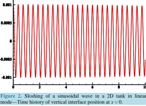
Figure 2shows the time history of vertical interface position during time in linear regime. The amplitude of the initial perturbation permits to stay within the framework of [28]. As viscous effects only damp the amplitude of the wave, inviscid simulations are performed, i.e. μ1 =μ1 = 0 and the diffusion term of momentum disappears from the equation of motion. The evolution in time is thus conditioned by the competition between the inertia of the fluid determined by the term
ρ
V⋅∇V and gravity source termρ
g. The latter term is not derived from a scalar potential and Hodge-Helmholtz decomposition of s=ρg= ∇Φ + ∇×s Ψs highlights two non-zero con-tributions thereof. The irrotational part modifies the scalar pressure potential P0 which includes the staticgravi-tational effects and the vector potential changes the mechanical equilibrium. Coupling with inertia causes the
Table 1. Natural convection in a differentially heated cavity for a Raleigh number of 105. The reference Nusselt number is obtained by Richardson extrapolation [27]. The value of the KSP method corres-pond to solution on a 10242 Cartesian mesh.
Reference N→ +∞ KSP N = 1024
Figure 2. Sloshing of a sinusoidal wave in a 2D tank in linear mode—Time history of vertical interface position at x = 0.
sloshing movement whose frequency may be calculated by the linear theory. If the initial disturbance of the in-terface is defined by Fourier modes, i in the longitudinal direction and j for transverse modes, the linear theory allows expressing the frequency [29]:
2 2 2 2
2 2 2 2
1
π π
2π
i j i j
f g th H
L l L l
= + +
(18)
where l is the width of the domain along y. In two-dimensions, j = 0 and l = 1. We also define the pulsation ω and period T:
2π 2πf .
T
ω= = (19)
The expression of the theoretical frequency (18) was established from a linear stability theory for a fluid den-sity ρ2 in the absence of fluid located above. When the densities ρ1 and ρ2 are close, it is necessary to introduce a correction [28] which gives the relationship:
2 2 2 2
2 1
2 2 2 2
2 1
1 π π
. 2π
i j i j
f g th H
L l L l
ρ ρ ρ ρ
−
= + +
+ (20)
Selected fluids are water and air and the corresponding densities are ρ2 = 1000 kg∙m−3 and ρ1 = 1.1728 kg∙m−3. Only the first 2D mode is tested, i.e. i = 1 and j = 1. The time step is equal to 10−3 s which achieves sufficient accuracy on the frequency of oscillations.Figure 2 shows the periodic changes in the height of the fluid 2 on one edge of the field x = 0. Gravitational forces introduce a downward movement of the area where the free sur-face is the highest. In the absence of viscous forces, the oscillatory motion is governed by the confrontation be-tween gravity and inertia. It is observed that the oscillations persist for a long time without significant attenua-tion. It is also to be noted that the wave attenuation is even lower as the time step decreases.
The present problem is used to test the entire methodology: the equation of motion, KSP time splitting algo-rithm, time and space discretization, interface tracking, etc. To quantify the errors introduced by the different modeling and discretization steps, frequency numerically obtained is compared with the theoretical frequency formulated by relation (18).Table 2 rather presents the period of the oscillations. There is a very good agree-ment between simulations and theory. This test validates the KSP approach in the presence of source terms such as gravity.
Figure 3. Sloshing of a sinusoidal wave in a 2D tank in non linear mode—initial interface shape (top left), interface solu-tion after 20 s (top right) and time history of vertical interface position for x = 0 m (bottom).
Table 2. Sloshing periods in a square cavity for the first li-near mode.
Theory Simulation
Period 0.3742 0.3748
3.4. Rotating Flow
The present test case corresponds to a solid rotating flow in a cylindrical cavity of radius R. The steady rotation-al velocity Ω0 is constant and the tangential component of absolute velocity is Va=vθ θe = Ω0reθ. The cavity is filled with two fluids of density ρ1 and ρ2 and the interface is initially located at r=R 2. The viscosity has no influence at least in the absence of differential motion relative to the plug flow. The flow motion can be treated in the moving frame relative to Oz axis. In the present configuration, the relative velocity V is chosen equal to zero in the whole domain. According to the momentum equations, the equation for pressure is given by
p
ρ
Ω×Ω× = −∇r (21) with Ω = ∇×V. The pressure can be calculated analytically and can then be compared with the numerical solu-tion:( )
2 2 02
r
p r = Ωρ +p (22) where p0 is a selected constant chosen equal to zero on the axis. Since the density is not constant in the whole
area, the pressure field will be calculated in the two fluid sub-domains on an analytical point of view. The KSP method is now applied from a zero velocity field V = 0 and a zero pressure field p = 0. Equations (2) applied to the problem gives the prediction velocity *
V which is not divergence free. This is a centrifugal velocity oriented outward as
* 2
0
t .r
= ∆ Ω
V (23) From that predicted velocity field, it is possible to apply the projection phase (3) for obtaining the scalar po-tential Φ of the velocity. However, in the present test case *
V is a gradient field from the potential Φ defined in a constant, *= ∇Φ
V that satisfies
2 0
.
t
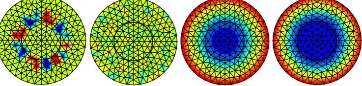
[image:9.595.199.426.356.392.2]As the theoretical solution is a polynomial of order two, it is expected that the numerical solution will be ac-curate. Indeed, all polynomial of order lower or equal to two can be represented exactly by a spatial discretiza-tion scheme of order equal to two. Solving the Poisson Equadiscretiza-tion (3) actually gives the expected result, as re-ported inFigure 4. As the projection is purely kinematics, the correction velocity VΦ = ∇Φ is completely con-tinuous and has no discontinuities at the interface between the two fluids. The numerical solution obtained with KSP at the end of the two stages is zero. The pressure is obtained from the Stokes formula (11) taking care to calculate the integral by piece if a segment Γ of a given mesh cell is intersected by the interface. Here the inter-face is known analytically and it is simple to specify the position of the intersection point on the segment. Not only the divergence of Vn+1 but also the velocity field itself are zero with the KSP method, in agreement with the expected analytical solution. This is not the case with standard projection methods that generate rotation ve-locity components that are non-physical. The solution to this problem was obtained with the KSP algorithm ac-curately regardless of the mesh type, i.e. structured or unstructured, in one time iteration consisting of a predic-tion step and a kinematics correcting step.
With classical scalar projection (SP) methods, the velocity is calculated from the pressure correction as
1 *
n
p t
ρ
+ = − ∇ ′
∆
V V . For flows with variable density, the divergence of this velocity is zero but its curl is not
zero anymore. Indeed, if ∇p′ is a gradient, p t
ρ ∇ ′
∆ is not. This is not consistent with what is obtained by
us-ing the prediction V* in KSP and its scalar potential Φ. For KSP, Vn+1=V*+ ∇Φ. As a consequence, the di-vergence and also the curl of n+1
V is zero for the rotation flow as expected theoretically. In the case where the velocities are large, this residual curl of SP is merged with that of the flow, but for low flow rates or for equili-brium situations like the case shown in this section, it is necessary that n+1
V is also a gradient field (rotation or example of a static drop under capillary effect) in order to satisfy equilibrium state. In all other two-phase cases, the SP numerical technology generates an artefact such as some spurious rotational and associated velocities.
4. Conclusion and Discussions
[image:10.595.131.500.561.649.2]The kinematics KSP projection method for solving the equation of incompressible fluid motion essentially solves various problems of incompressible flows, including flows with significant density variations. Unlike conventional methods where the pressure is first calculated from a Poisson equation with variable coefficients, the irrotational velocity is calculated first in KSP. The scalar potential of velocity is then obtained by solving a Poisson problem with constant coefficients that is insensitive to density variations. The scalar potential of the amount of acceleration, i.e. the pressure, is obtained thanks to the Stokes’ theorem by introducing at this stage the local density. In terms of accuracy in time and space, the results are very close to those of the conventional projection methodology for flows at variable density. However, the large variations in density introduce local consistency defects in standard projection methods due to interpolation of density at the location of each com-ponent of the velocity. The pressure undergoes non-physical variations that can lead to unstable or non-physical behaviors. The KSP method allows finding consistency between the pressure and the local density. This method
Figure 4. Comparison between the scalar projection (SP) and the kinematic scalar projection (KSP) on a triangular unstructured mesh. From left to right are represented the rotationnal of velocity for classical scalar projection (SP) with ∇ × ±V 0.1, the rotationnal of velocity KSP method with
15
10−
can be interpreted as a simple splitting of the motion equation of the continuum mechanics previously discre-tized in time. It is based on an original formulation of the law for fluid dynamics written as a discrete Helm-holtz-Hodge decomposition.
The proposed KSP time splitting approach satisfies the following properties:
• The continuous media properties of differential operators, i.e. ∇×∇Φ =0 and ∇ ⋅∇ ×Ψ=0, are satisfied to almost computer error.
• The space convergence order is 2 with a centered scheme and the time convergence order can be 1 or 2 de-pending on the order of the Taylor expansion used for the time derivative of the momentum conservation equations.
• The numerical solution is exact whatever the mesh for all theoretical solution of order equal or less than 2.
• KSP as SP are a prediction-correction method whose artifacts are well known, i.e. artificial boundary layers are generated by the projection step near the boundaries. Their magnitude decreases during time iterations.
• Unlike conventional projection methods, the resolution steps for pressure and velocity are reversed. The scalar potential of the velocity Φ is first obtained and then the physical potential, i.e. the pressure, is updated explicitly and accurately.
• The Poisson equation for velocity potential is at constant coefficients and the velocity potential does not de-pend on density.
• The solving of the linear system is easy and allows the use of existing efficient parallel solvers.
As a conclusion, the KSP method is, among those existing in the literature, the easiest method to implement since it consists in solving a Poisson equation with constant coefficients.
References
[1] Fortin, M. and Glowinski, R. (1982) Méthodes de lagrangien augmenté, application à la résolution numérique de problèmes aux limites. Dunod, Paris.
[2] Vincent, S., Sarthou, A., Caltagirone, J.-P., Sonilhac, F., Février, P., Mignot, C. and Pianet, G. (2011) Augmented La-grangian and Penalty Methods for the Simulation of Two-Phase Flows Interacting with Moving Solids. Application to Hydroplaning Flows Interacting with Real Tire Tread Patterns. Journal of Computational Physics, 230, 956-983. http://dx.doi.org/10.1016/j.jcp.2010.10.006
[3] Chorin, A.J. (1968) Numerical Solution of the Navier-Stokes Equations. Mathematics of Computation, 22, 745-762. http://dx.doi.org/10.1090/S0025-5718-1968-0242392-2
[4] Rhie, C.M. and Chow, W.L. (1983) Numerical Study of the Turbulent Flow past an Airfoil with Trailing Edge Sepa- ration. AIAA Journal, 21, 1525-1532. http://dx.doi.org/10.2514/3.8284
[5] Harlow, F.H. and Welch, J.E. (1965) Numerical Calculation of Time-Dependent Viscous Incompressible Flow of Fluid with a Free Surface. Physics of Fluids, 8, 2182-2189. http://dx.doi.org/10.1063/1.1761178
[6] Guermond, J.L., Minev, P. and Shen, J. (2006) An Overview of Projection Methods for Incompressible Flows. Com- puter Methods in Applied Mechanics and Engineering, 195, 6011-6045. http://dx.doi.org/10.1016/j.cma.2005.10.010 [7] Bell, J.B., Colella, P. and Glaz, H.M. (1989) A Second Order Projection Method for the Incompressible Navier-Stokes
Equations. Journal of Computational Physics, 85, 257-283. http://dx.doi.org/10.1016/0021-9991(89)90151-4
[8] Benzi, M. (2002) Preconditioning Techniques for Large Linear Systems: A Survey. Journal of Computational Physics, 182, 418-477. http://dx.doi.org/10.1006/jcph.2002.7176
[9] Benzi, M., Golub, G.H. and Liesen, J. (2005) Numerical Solution of Saddle Point Problems. Acta Numerica, 14, 1-137. http://dx.doi.org/10.1017/S0962492904000212
[10] Cai, M., Nokaka, Y., Bell, J.B., Griffith, B.E. and Donev, A. (2014) Efficient Variable-Coefficient Finite-Volume Stokes Solvers. Numerical Analysis, 327, 1179-1184.
[11] Guermond, J.L. and Salgado, A. (2009) A Splitting Method for Incompressible Flows with Variable Density Based on a Pressure Poisson Equation. Journal of Computational Physics, 228, 2834-2846.
http://dx.doi.org/10.1016/j.jcp.2008.12.036
[12] Liu, C., Shen, J. and Yang, X.F. (2015) Decoupled, Energy Stable Schemes for Phase-Field Models of Two-Phase In-compressible Flows. Journal of Scientific Computing, 62, 601-622. http://dx.doi.org/10.1007/s10915-014-9867-4 [13] Poux, A., Glockner, S. and Azaïez, M. (2011) Improvements on Open and Traction Boundary Conditions for Navier-
Stokes Time-Splitting Methods. Journal of Computational Physics, 230, 4011-4027. http://dx.doi.org/10.1016/j.jcp.2011.02.024
of Computational Physics, 273, 416-434. http://dx.doi.org/10.1016/j.jcp.2014.05.024
[15] Caltagirone, J.-P. and Vincent, S. (1999) Sur une méthode de pénalisation tensorielle pour la résolution des équations de Navier-Stokes. Comptes Rendus de l’Académie des Sciences Série IIb, 329, 607-613.
http://dx.doi.org/10.1016/S1620-7742(01)01374-5
[16] Angot, P., Caltagirone, J.-P. and Fabrie, P. (2012) A Fast Vector Penalty-Projection Method for Incompressible Non- Homogeneous or Multiphase Navier-Stokes Problems. Applied Mathematics Letters, 25, 1681-1688.
http://dx.doi.org/10.1016/j.aml.2012.01.037
[17] Angot, P., Caltagirone, J.-P. and Fabrie, P. (2013) Fast Discrete Helmholtz-Hodge Decompositions in Bounded Do-mains. Applied Mathematics Letters, 26, 445-451. http://dx.doi.org/10.1016/j.aml.2012.11.006
[18] Lemoine, A., Caltagirone, J.-P., Azaiez, P. and Vincent, S. (2014) Discrete Helmholtz-Hodge Decomposition on Poly-hedral Meshes Using Compatible Discrete Operators. Journal of Scientific Computing.
http://dx.doi.org/10.1007/s10915-014-9952-8
[19] Bhatia, H., Norgard, G., Pascucci, V. and Bremer, P.T. (2012) The Helmholtz-Hodge Decomposition—A Survey.
IEEE Transactions on Visualization and Computer Graphics, 99, 1386-1404. [20] Caltagirone, J.-P. (2015) Discrete Mechanics. ISTE, John Wiley & Sons, London.
http://dx.doi.org/10.1002/9781119058588
[21] Caltagirone, J.-P. (2015) Application de la décomposition de Hodge-Helmholtz discrète aux écoulements incompressibles.
HAL,1-11. https://hal.archives-ouvertes.fr/hal-01099958
[22] Peyret, R. and Taylor, T.D. (1983) Computational Methods for Fluid Flow. Springer-Verlag, New York.
[23] Trontin, P., Vincent, S., Estivalezes, J.-L. and Caltagirone, J.-P. (2012) A Subgrid Computation of the Curvature by a Particle/Level-Set Method. Application to a Front-Tracking/Ghost-Fluid Method for Incompressible Flows. Journal of Computational Physics, 231, 6990-7010. http://dx.doi.org/10.1016/j.jcp.2012.07.002
[24] Vincent, S., Balmigère, G., Caltagirone, J.-P. and Meillot, E. (2010) Eulerian-Lagrangian Multiscale Methods for Solving Scalar Equations—Application to Incompressible Two-Phase Flows. Journal of Computational Physics, 229, 73-106. http://dx.doi.org/10.1016/j.jcp.2009.09.007
[25] Vincent, S., Caltagirone, J.-P., Lubin, P. and Randrianarivelo, T.N. (2004) An Adaptative Augmented Lagrangian Me-thod for Three-Dimensional Multimaterial Flows. Computers and Fluids, 33, 1273-1279.
http://dx.doi.org/10.1016/j.compfluid.2004.01.002
[26] Vincent, S. and Caltagirone, J.-P. (2000) Numerical Solving of Incompressible Navier-Stokes Equations Using an Original Local Multigrid Refinement Method. Comptes Rendus de l’Académie des Sciences SérieIIb, 328, 73-80. http://dx.doi.org/10.1016/s1287-4620(00)88419-7
[27] Richardson, L.F. and Gaunt, J.A. (1927) The Deferred Approach to the Limit. Philosophical Transactions of the Royal Society A, 226, 299-349. http://dx.doi.org/10.1098/rsta.1927.0008