http://dx.doi.org/10.4236/jamp.2015.37100
Sniffer Technique for Numerical Solution of
Korteweg-de Vries Equation Using Genetic
Algorithm
Dilip P. Ahalpara
Department of Master of Computer Applications, D.D. University, Nadiad, India Email: [email protected]
Received 6 May 2015; accepted 23 June 2015; published 30 June 2015
Abstract
A novel heuristic technique has been developed for solving Ordinary Differential Equation (ODE) numerically under the framework of Genetic Algorithm (GA). The method incorporates a sniffer procedure that helps carry out a memetic search within the solution domain in the vicinity of the currently found best chromosome. The technique has been successfully applied to the Korteweg- de Vries (KdV) equation, a well-known nonlinear Partial Differential Equation (PDE). In the pre- sent study we consider its solution in the regime of solitary waves, or solitons that is first used to convert the PDE into an ODE. It is then shown that using the sniffer technique assisted GA proce-dure, numerical solution has successfully been generated quite efficiently for the one-dimen- sional ODE version of the KdV equation in space variable (x). The technique is quite promising for its applications to systems involving ODE equations where analytical solutions are not directly available.
Keywords
Sniffer Technique, Genetic Algorithm, Numerical Solution of ODE, Evolutionary Computation
1. Introduction
experimental data by Cao et al. [7] and Iba et al. [8].
In the present paper, we first consider the well known Korteweg-de Vries (KdV) equation which is a nonli-near PDE involving two independent variables in space x and time t, and is highly studied in literature since the discovery of its soliton solution by Zabusky and Kruskal [9],
3
3
6 0
t x x
∂Φ+ Φ∂Φ ∂ Φ+ =
∂ ∂ ∂ (1)
It is known that considering a traveling wave given by Φ
( )
x t, = Ψ −(x ct), where c is phase velocity, the PDE can be converted to an ODE using a new independent variable ξ = −x ct3
3
6 0
d d d
c
dξ dξ dξ
Ψ Ψ Ψ
− + Ψ + = (2)
and integrating with respect to ξ, the ODE assumes a simpler form with which we will work henceforth., 2 2 2 3 d c A dξ Ψ
− Ψ + Ψ + = (3)
where A is an arbitrary constant of integration. Here, when x→ ±∞ it is required that Ψ →0 and
0
d dξ
Ψ→
.
The KdV equation is known to have an analytical solution of the form
( )
2, [ ( )]
2 2
c c
x t Sech x ct a
Ψ = − − (4)
[image:2.595.95.535.157.378.2] [image:2.595.184.454.491.698.2]Setting a = 0, c = 1.2 and t = 0 now onwards, the true solution of KdV equation in one dimension is shown in Figure 1, where we have chosen even-spaced discrete x-values in the range [−4.0, 4.0] and even-spaced discrete y-values in the range [0.0, 0.7] incorporating N grid points both in the x and y axes within the solution domain, where N is chosen as51.The chromosome representation therefore is having a linear structure of a list having N elements, and each element is a whole number bounded within the range [1, N], as will be exemplified in Sec-tion 1.2 later.
Next we consider GA algorithm to get the solution sketched in Figure 1 numerically, without having apriori knowledge of its analytical solution. For this, we first define a fitness function as,
2 2
2 1
( ) N ( 3 i) /
i i
i
d
Fitness c N A
dx =
Ψ
Ψ =
∑
− Ψ + Ψ + − (5)where, N is the number of grid points considered, Ψ = Ψi ( )xi and A is a constant of integration to be de-scribed shortly. In order to calculate numerical values for the 2nd derivative in equation (5), we use the standard five-point formula based on central difference that gives very good approximations to the numerical derivatives.
The fitness value for the true solution as given by Equation (5) is 0.4802-A, where the departure from -A is due to the discretized solution domain considered (resulting in chromosome representation by whole numbers in range [1, N]), as well as due to the numerical inaccuracy in calculating the derivative values. We then set A = 0.4802 so as to offset the fitness measure such that it assumes the ideal value 0 for the true solution. Thus any solution that has departure from the true solution is expected to give fitness measure > 0. It may be emphasized that any other choice of value for A does not affect the GA search procedure.
1.1. Heuristic Methods for Solving One-Dimensional KdV Equation
We now consider one-dimensional KdV Equation (3) and proceed to solve it numerically. Combinatorially the search space is quite complex, due to the fact that a given linear chromosome, having a list of 51 integers, can have 51 independent possible values for each element. The standard GA is found to be quite slow in making progress for converging towards the ideal value of 0. In this scenario, it is envisaged to apply a heuristic search in the local surrounding area of the currently found best solution during GP iteration. The sniffing around the best solution is aimed at making the GA search procedure more effective. In order to define a numerical measure for the locality of search, a sniffer radius denoted by εsniffer is considered, which forms a maximum bound within which local search is carried out. It is emphasized here that the sniffer technique considered is purely as an aid to the standard GA procedure and it certainly can not replace it. Hand in hand, they both work together to improve the overall search efficiency. On one hand GA iterations bring about a variety of candidate solutions (as is required for not getting trapped in a local minima), and on top of this basic search procedure, the sniffer tech-nique helps carry out a stochastic (and not an exhaustive) local search in the vicinity of the best solution achieved so far by the GP procedure. This is explained by a schematic diagram in Figure 2. It may be noted that we have earlier applied the sniffer technique [10] for solving the inverse problem, namely inference of dynami-cal system equations (ODE and PDE) in their symbolic form, where data is used in the form of its solution de-fined either numerically or in a symbolic form.
Figure 2 shows a hypothetical search space in which the true solution is shown by an isolated thick circle. The remaining thick circles surrounded by small circles represent the best solution found by GA at various in-stances during the search iteration. Tiny dots spread randomly within these small circles represent the search carried out by the heuristic sniffer method. The radius of these small circles denote the sniffer radius εsniffer. It is seen that the sniffer technique thus tries out searching in the vicinity of the best solution within a small region governed by sniffer radius. When the GA search procedure locates a solution close enough within the reach of sniffer radius to the true solution, the local search is quite likely to find the true solution through the sniffer technique. Different heuristic sniffer methods implemented in this technique are described below.
[image:3.595.225.399.555.695.2]It may be noted that during the heuristic search the boundary values Ψ( )x1 and Ψ(xN) are kept fixed at given constant values and only the rest of Ψ( )xi values for i = 2 to N − 1 are varied during heuristic as well as
GA search. In the present GA experiments these boundary values are kept at 2 within the possible range of [1, N]. Sniff1 and Sniff2 methods descried below vary Ψ( )xi values within the bounds of sniffer radius to check whether the best solution can be improved in its locality. WhereasSniff1 varies all the Ψ( )xi values, Sniff2 va-ries a group of contiguous Ψ( )xi values. Sniff3 and Sniff4are their refined variants.
o Sniff1: Each of the Ψ( )xi value is added and subtracted separately by a random number bounded by sniffer radius, to get modified chromosomes Ψ1( )xi and Ψ2( )xi respectively; whichever of these two chromo-somes gives improved fitness is selected.
o Sniff2: A contiguous range, specified by x1 to x2(selected randomly) and the corresponding Ψ( )xi values are added and subtracted separately by a random number, bounded by sniffer radius, to get modified chro-mosomes Ψ1( )xi and Ψ2( )xi ; whichever of these two solutions gives improved fitness is selected. o Sniff3: A contiguous range, specified by x1 to x2 (selected randomly) and corresponding Ψ( )xi values are
added and subtracted separately by a random number bounded by sniffer radius. The modified list of Ψ( )xi
values is then fitted by using a polynomial function up to nth degree to obtain a smooth function passing through the perturbed Ψ( )xi values. We have chosen n = 4. The interpolated function values at successive xi values are then taken as the modified chromosomes Ψ1( )xi and Ψ2( )xi ; whichever of these two chro-mosomes gives improved fitness is selected.
o Sniff4: A list of good points within the chromosome list are identified corresponding to individual fitness components (right side of Equation (5) at given value i) by checking that it is less than a pre-specified frac-tion of fitness value. Once the list of these good points is obtained, a polynomial function Pn(x) (i.e. up to order xn, where n is set to 4), is then passed through these points. The chromosome values are then replaced by interpolated values as given by Pn(x).
1.2. Genetic Algorithm Framework
Based on the pioneering work by David Goldberg [11], the basic framework of Genetic Algorithm is considered as an engine to discover various solution regimes stochastically and by natural selection principle. Considering the fitness measure as given by equation (5), GA based iterative search is carried out using a code developed in-digenously in Mathematica. As shown in Figure 1, the solution domain [{−4, 4}, {0.0, 0.7}] for [x, y] range is mapped on to a corresponding grid [{1, N}, {1, N}], where we have chosen N = 51. Each chromosome is thus an integer list of length N representing successive grid point numbers in the range [1, N] corresponding to the
( )xi
Ψ values rounded to nearest grid point. The true solution for example, as given by equation (4), with a = 0, c = 1.2 and t = 0, corresponds to the chromosome {2, 2, 3, 4, 5, 6, 7, 8, 9, 11, 13, 15, 17, 20, 23, 26, 29, 32, 36, 39, 42, 45, 48, 49, 51, 51, 51, 49, 48, 45, 42, 39, 36, 32, 29, 26, 23, 20, 17, 15, 13, 11, 9, 8, 7, 6, 5, 4, 3, 2, 2} having the fitness measure as 0.
The search procedure for finding the best chromosome having smallest fitness value is carried out as follows, 1. A pool of chromosomes is created having individuals that are stochastically generated representing candidate
solutions
2. Iterations are carried out till an acceptable solution is obtained (having fitness value smaller then a specified small value, or maximum number of iterations have been achieved)
o The fitness values for the candidate chromosomes are calculated
o Standard genetic operators (copy, crossover and mutation) are applied on the pool of chromosomes to evolve the given population to anew population, hopefully containing a better pool of candidate chromosomes. Few (at least 1) elite solutions are preserved (without any change) so as not to loose the best chromosomes dis-covered so far during the iterative search.
o Sniffer functions (Sniff1 to Sniff4) are activated intermittently after the GA iterations relax for a specified number of n iterations (we have chosen n = 10)
3. The best solution obtained represents the solution of the problem
The parameters used for the GA experiments are shown in Table 1, using which the KdV Equation (3) is solved numerically in the next section.
2. Results of GA Experiments
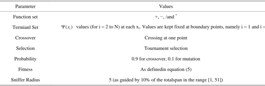
Table 1. Parameters used for the GA search procedure.
Parameter Values
Function set +, −, /and *
Termianl Set Ψ( )xi values (for i = 2 to N) at each xi. Values are kept fixed at boundary points, namely i = 1 and i = N.
Crossover Crossing at one point
Selection Tournament selection
Probability 0.9 for crossover, 0.1 for mutation
Fitness As definedin equation (5)
Sniffer Radius 5 (as guided by 10% of the totalspan in the range [1, 51])
cedure aided by the sniffer technique. The GA solutions along with the templates used are shown below. Thus the inclusion of various template curves as one of the chromosomes is aimed at trying out different useful chro-mosome structures as potential candidates during the GA solutions.
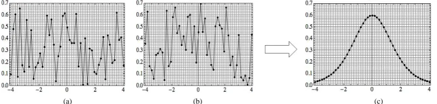
2.1. Single Bump Symmetric Templates
As shown in Figure 3, two symmetric template curves (triangular (a) and a square like bump (b)) are used that generate an exact solution (c) with fitness value as 0.Here the GA iterations were monitored to find the effec-tiveness of sniffer technique. This analysis indicated that the percentage of iterations in which sniffer methods were successful in improving the fitness value as compared to GA iterations were 74% in case of GA experi-ment using the profile of Figure 3(a), and it was 83% in case of profile of Figure 3(b).
2.2. Single Bump Asymmetric Templates
As shown in Figure 4, two asymmetric template curves (triangular curves leaning forward (a) and leaning backward (b)) are used and in both cases the exact solution (c) is generated.
2.3. Randomly Generated Templates
As shown in Figure 5, totally random templates (a) and (b) are used, and in both cases the exact solution (c) is generated.
It is interesting to note that in all above GA experiments, the best solution generated by sniffer assisted GA algorithm matches exactly with the true solution having fitness measure as 0.
2.4. Sensitivity on Fitness Measure
In order to check the sensitivity of the best solution obtained by GA, we next test the sensitivity of fitness meas-ure as a result of applying small perturbations in the best chromosome structmeas-ure. We consider following two scenarios and calculate fitness measure 1000 times and then taking the average,
1. Perturbing Ψ( )xi values corresponding to two randomly selected xi values except at the end points. 2. Perturbing Ψ( )xi values corresponding to all xi values except at the end points.
In the first scenario, the average variation in fitness measure is found to be 0.172, 0.203 and 0.526 for pertur-bation values as 1, 2 and 5 respectively. In the second scenario, the average variation in fitness measure is found to be 1.195, 2.284 and 5.675 for perturbation values 1, 2 and 5 respectively.
[image:6.595.94.536.83.186.2]
(a) (b) (c)
Figure 3. GA solution (c) obtained using the triangular (a) and square bump (b) symmetric templates.
[image:6.595.102.534.217.323.2]
(a) (b) (c)
Figure 4. GA solution (c) obtained using the triangular asymmetric templates (a) and (b) respectively.
(a) (b) (c)
Figure 5. GA solution (c) obtained using the randomly generated templates (a) and (b).
3. Conclusion and Outlook
It has been shown that the sniffer technique assisted Genetic Algorithm approach is quite useful in solving one- dimensional KdV equation. In the present paper the numerical solutions have successfully been obtained for the well-known KdV differential equation in one dimension. The search method implements several useful variants of a novel heuristic method, called sniffer technique that helps make a detailed search in the vicinity of the best solution achieved by GA at a given instance during its iterations. The method would especially be useful for solving stiff as well as complex differential equations for which no analytical solutions exist. Work is in progress for generating numerical solution for the ODE equations in two dimensions (involving space and time), of the type in Equation (1), using which it would be interesting to generate time evolution of 1-soliton as well as 2-soliton profiles fed at time t = 0.
References
[1] Seaton, T., Brown, G. and Miller, J.F. (2010) Analytical Solution to Differential Equations under Graph-Based Genetic Programming. Lecture Notes in Computer Science, 6021, 232-243. http://dx.doi.org/10.1007/978-3-642-12148-7_20
[2] Butcher, J.C. (2008) Numerical Methods for Ordinary Differential Equations. 2nd Edition, John Wiley Publication.
http://dx.doi.org/10.1002/9780470753767
[image:6.595.92.539.354.461.2][4] Lambert, J.D. (1991) Numerical Methods for Ordinary Differential Systems: The Initial Value Problem, John Wiley and Sons, Chichester, England.
[5] Fasshauer, G.E. (1999) Solving Differential Equations with Radial Basis Functions: Multilevel Methods and Smooth-ing. Advances in Computational Mathematics, 11, 139-159. http://dx.doi.org/10.1023/A:1018919824891
[6] Lagaris, I., Likas A., and Fotiadis D.I. (1998) Artificial Neural Networks for Solving Ordinary and Partial Differential Equations. IEEE Transactions on Neural Networks, 9, 987-1000. http://dx.doi.org/10.1109/72.712178
[7] Cao, H., Kang, L., Chen, Y. and Yu, J. (2000) Evolutionary Modeling of Systems of Ordinary Differential Equations with Genetic Programming. Genetic Programming and Evolvable Machines, 1, 309-337.
http://dx.doi.org/10.1023/A:1010013106294
[8] Iba, H. and Sakamoto, E. (2002) Inference of Differential Models by Genetic Programming. Proceedings of the Genet-ic and Evolutionary Computation Conference (GECCO), 788-795.
[9] Zabusky, N.J. and Kruskal, M.D. (1965) Interaction of Solitons in a Collisionless Plasma and the Recurrence of Initial States. Physical Review Letters, 15, 240-243. http://dx.doi.org/10.1103/PhysRevLett.15.240
[10] Ahalpara, D.P. and Sen, A. (2011) A Sniffer Technique for an Efficient Deduction of Model Dynamcal Equations us-ing Genetic Programmus-ing. Proceedings of the 14th European Conference on Genetic Programming, EuroGP, Torino. Lecture Notes in Computer Science (LNCS), 6621, 1-12. http://dx.doi.org/10.1007/978-3-642-20407-4_1
![Figure 1, where we have chosen even-spaced discrete x-values in the range [−4.0, 4.0] and even-spaced discrete y-values in the range [0.0, 0.7] incorporating N grid points both in the x and y axes within the solution domain, where N is chosen as51.The chromosome representation therefore is having a linear structure of a list having N](https://thumb-us.123doks.com/thumbv2/123dok_us/8104971.789084/2.595.184.454.491.698/figure-discrete-discrete-incorporating-solution-chromosome-representation-structure.webp)