Predictability and Model Selection in the Context of ARCH Models

Predictability and Model Selection in the

Context of ARCH Models

Degiannakis, Stavros and Xekalaki, Evdokia

Department of Statistics, Athens University of Economics and

Business

2005

Online at

https://mpra.ub.uni-muenchen.de/80486/

P r e d i c t a b i l i t y a n d M o d e l S e l e c t i o n i n t h e

C o n t e x t o f A R C H M o d e l s

Stavros Degiannakis and Evdokia Xekalaki

Department of Statistics, Athens University of Economics and Business

Abstract

Most of the methods used in the ARCH literature for selecting the appropriate model are based on evaluating the ability of the models to describe the data. An alternative model selection approach is examined based on the evaluation of the predictability of the models in terms of standardized prediction errors.

1 . I n t r o d u c t i o n

ARCH models have widely been used in financial time series analysis, particularly in analyzing the risk of holding an asset, evaluating the price of an option, forecasting time varying confidence intervals and obtaining more efficient estimators under the existence of heteroscedasticity.

In the recent literature, numerous parametric specifications of ARCH models have been considered for the description of the characteristics of financial markets. In the linear ARCH(q) model, originally introduced by Engle (1982), the conditional variance is postulated to be a linear function of the past q squared innovations. Bollerslev (1986) proposed the generalized ARCH, or GARCH(p,q), model, where the conditional variance is postulated to be a linear function of both the past q squared innovations and the past p conditional variances. Nelson (1991) proposed the exponential GARCH, or EGARCH, model. The EGARCH model belongs to the family of asymmetric GARCH models, which capture the phenomenon that negative returns predict higher volatility than positive returns of the same magnitude. Other popular asymmetric models are the GJR model of Glosten et al. (1993), the threshold GARCH, or TARCH, model, introduced by Zakoian (1990) and the quadratic ARCH, or QGARCH, model, introduced by Sentana (1995). ARCH models go by such exotic names as AARCH, NARCH, PARCH, PNP-ARCH and STARCH among others. For a comprehensive review of the literature on such models, the interested reader is referred to Degiannakis and Xekalaki (2004).

The richness of the family of parametric ARCH models certainly complicates the search for the true model, and leaves quite a bit of arbitrariness in the model selection stage. The problem of selecting the model that describes best the movement of the series under study is, therefore, of practical importance.

1996, while, in section 6, a selection method based on the ability of the models describing the data is investigated. Finally, in section 7, a brief discussion of the results is provided.

2 . T h e A R C H P r o c e s s

Let



yt

 





_t1 refer to the univariate discrete time real-valued stochastic process to

be predicted (e.g. the rate of return of a particular stock or market portfolio from time

t



1

to

t

) where



is a vector of unknown parameters and E



yt

 



|It1



 Et1



yt

 









t

 



denotes the conditional mean given the information set available at time

t



1

, It_1. The

innovation process for the conditional mean,





t

 





_t1, is then represented by

 



 





 





t  yt  t with corresponding unconditional variance

 















2

 









2

 



t

t

E

V

, zero unconditional mean and E





t

   





s





0,



t



s

. The conditional variance of the process given It1 is defined by

 









 









2

 







2

 



1

1 1

|

t t t t t t

t

I

V

y

E

y

V

_



_



_



. Since investors would know the

information set It_1 when they make their investment decisions at time

t



1

, the relevant

expected return to the investors and volatility are



_t

 



and



_t2

 



, respectively.

An ARCH process,





t

 





_t1, can be presented as:

 

 

 

 

 

 





 



 

,

 

,...;

 

,

 

,...;

,

,...



,

1

,

0

~

2 1 2

1 2

1 2

. . .

  

 

















t t t

t t

t t

t t

d i i

t

t t t

t t t

g

z

V

z

E

f

z

z

x

y









































(2.1)

where x_t is a

k



1

vector of endogenous and exogenous explanatory variables included in the information set It_1,



is a

k



1

vector of unknown parameters,

f

 

.

is the density

function of zt,



t

 



is a time-varying, positive and measurable function of the

information set at time

t



1

,



t is a vector of predetermined variables included in It, and



.

g

is a linear or nonlinear functional form. By definition,



_t

 



is serially uncorrelated

with mean zero, but with a time varying conditional variance equal to



t2

 



. The standard

Bollerslev (1987) proposed using the student t distribution with an estimated kurtosis regulated by the degrees of freedom parameter. Nelson (1991) proposed the use of the generalized error distribution (Harvey (1981), Box and Tiao (1973)), which is also referred to as the exponential power distribution. Other distributions, that have been employed, include the generalized t distribution (Bollerslev et al. (1994)), the normal Poisson mixture distribution (Jorion (1988)), the normal lognormal mixture (Hsieh (1989)), and a serially dependent mixture of normally distributed variables (Cai (1994)) or student t distributed variables (Hamilton and Susmel (1994)). In the sequel, for notational convenience, no explicit indication of the dependence on the vector of parameters,



, is given when obvious from the context.

Let us assume that the conditional mean,



t E



yt |It₁



, can be adequately

described by a



th order autoregressive



AR

 





model:





t

i

i t i

t c c y

y





 





1 

0 . (2.2)

Usually, the conditional mean is either the overall mean or a first order autoregressive

process. Theoretically, the

AR

 

1

process allows for the autocorrelation induced by discontinuous (or non-synchronous) trading in the stocks making up an index (Scholes and Williams (1977), Lo and MacKinlay (1988)). According to Campbell et al. (1997), “the non-synchronous trading arises when time series, usually asset prices, are taken to be recorded at time intervals of a fixed length when in fact they are recorded at time intervals of other, possible irregular lengths.” The Scholes and Williams model suggests the st

1 order moving average process for index returns, while the Lo and MacKinlay model

suggests an

AR

 

1

form. Higher orders of the autoregressive process are considered in order to investigate if they are adequate to produce more accurate predictions.

Engle (1982) introduced the original form of



_t2



g



.

as a linear function of the past q squared innovations:







 



 q

i

i t i

t a a

1 2 0

2





. (2.3)

For the conditional variance to be positive, the parameters must satisfy



0 0,ai 0, for

q





_







 

 

 

 p

i

i t i q

i

i t i

t a a b

1 2 1

2 0

2







, (2.4)

where



0 0,ai 0, for

i



1

,...,

q

, and bi 0, for

i



1

,...,

p

. Note that even though the

innovation process for the conditional mean is serially uncorrelated, it is not independent through time. The innovations for the variance are denoted as:

 

t t

 

t t t t

t

E

v

E



2



_1



2





2





2



. (2.5) The innovation process

 

v_t is a martingale difference sequence in the sense that it cannot be predicted from its past. However, its range may depend upon the past, making it neither serially independent nor identically distributed.

The GARCH(p,q) model successfully captures several characteristics of financial time series, such as thick tailed returns and volatility clustering first noted by Mandelbrot (1963): “… large changes tend to be followed by large changes of either sign, and small changes tend to be followed by small changes…”. On the other hand, the GARCH structure imposes important limitations. The variance only depends on the magnitude and

not on the sign of



_t, which is somewhat at odds with the empirical behavior of stock

market prices where a leverage effect may be present. The term leverage effect, first noted by Black (1976), refers to the tendency for changes in stock returns to be negatively correlated with changes in returns volatility, i.e. volatility tends to rise in response to bad

news,





t 0



, and to fall in response to good news,





t 0



.

In order to capture the asymmetry exhibited by the data, a new class of models was introduced, termed the asymmetric ARCH models. The most popular model proposed to capture the asymmetric effects is Nelson’s (1991) exponential GARCH, or EGARCH(p,q), model:

 

_

_



 



 

 





 _

    

  

       

 p

i

i t i q

i t i

i t i i t

i t i

t a a b

1

2 1

0 2

ln

ln















. (2.6)









_







 

 

 

  



 p

i

i t i t

t q

i

i t i

t a a d b

1 1

1 1

0 0

 





_

_

_

_

_



, (2.7)

where d





t 0



1 if



t 0, and d





t 0



0 otherwise. Zakoian’s (1990) model is a

special case of the TARCH model with





1

, while Glosten et al. (1993) consider a version of the TARCH model with





2

. The TARCH model allows a response of volatility to news with different coefficients for good and bad news.

A wide range of ARCH models proposed in the literature has been reviewed by Bera and Higgins (1993), Bollerslev et al. (1992), Bollerslev et al. (1994), Degiannakis and Xekalaki (2004), Gourieroux (1997) and Hamilton (1994).

3 . M o d e l S e l e c t i o n M e t h o d s

Most of the methods used in the literature for selecting the appropriate model are based on evaluating the ability of the models to describe the data. Standard model selection criteria such as the Akaike Information Criterion (AIC) (Akaike (1973)) and the Schwarz Bayesian Criterion (SBC) (Schwarz (1978)) have widely been used in the ARCH literature, despite the fact that their statistical properties in the ARCH context are

unknown. These are defined in terms of

l

_T

 



ˆ

, the maximized value of the log-likelihood function of a model, where



ˆ

is the maximum likelihood estimator of



based on a sample of size T and





denotes the dimension of



, thus:

 











l

_T

ˆ

AIC

(3.1)

 

ˆ

2

1

ln

 

T

.

l

SBC



_T











(3.2)

In addition, the evaluation of loss functions for alternative models is mainly used in model selection. When we focus on estimation of means, the loss function of choice is typically the mean squared error (MSE):



 

 T

t t

T MSE

1 2 1



. (3.3)





,

1

2 2 2 1





  T

t

t t

L





(3.4)

,

ln

1

2 2 2

2



















T

t t

t

L





(3.5)





,

1

4 2 2 2

3









T

t t

t t

L







(3.6)

 

.

ln

1

2 2

2

4





















T

t

t t

t

L







(3.7)

Pagan and Schwert (1990) used the first two of the loss functions to compare alternative estimators with in-sample and out-of-sample data sets. Andersen et al. (1999), Heynen and Kat (1994), Hol and Koopman (2000), are some examples from the literature that applied loss functions to compare the forecast performance of various volatility models.

Moreover, loss functions have been constructed, based upon the goals of the particular application. West et al. (1993) developed such a criterion based on the portfolio decisions of a risk averse investor. Engle et al. (1993) assumed that the objective was to price options and developed a loss function from the profitability of a particular trading strategy.

4 . M o d e l S e l e c t i o n B a s e d o n t h e S t a n d a r d i z e d P r e d i c t i o n

E r r o r C r i t e r i o n ( S P E C )

Let us assume that a researcher is interested in evaluating the ability of the ARCH models to forecast the conditional variance. Consider the simple case of a regression

model: y_t  x_t







_t where



is a vector of

k

unknown parameters to be estimated, x_t

is a vector of explanatory variables included in the information set at time

t



1

and



2



. . .

, 0

~





N

d i i

t . At time

t



1

, the expected value



t of yt is estimated on the basis of the

information available at time

t



1

, i.e.

y

ˆ

_t|t1





ˆ

_t



x



_t



ˆ

_t1, where



 

1 1



1 1 1 1

ˆ  _{ }

 

  t t t t

t X X X Y



is the least square estimator of



at time

t



1

, Y_t is the



lt1



vector of lt observations on the dependent variable yt, and Xt is the



ltk



included in the information set, so that

_

















t t t

x

1

X

X

,

_















t t t

y

1

Y

Y

. Here l0 k, lt1 lt 1

and XtXt 0,

t



0

,

1

,...

. In a manner of speaking, yˆt|t and yˆt|t1 can be considered as

in-sample and out-of-sample forecasts, respectively. In other words, yˆ_t|t is measured on the basis of It, the information set available at time

t

, while yˆt|t1 is measured on the

basis of I_t1, the information set available at time

t



1

.

In the sequel, the density function

f

 

.

, in equation (2.1), is assumed to be that of

the normal distribution and ˆ| 1 ˆ| 1ˆ |11

     tt tt t

t

z





denotes the standardized one step ahead prediction errors1. The most commonly used way to model the conditional variance is the GARCH(p,q) process in (2.4). The GARCH(p,q) process may be rewritten as2:















_t2



u



_t

,

_t



,

w

_t



v

,

,

,

where ut



1,



t2₁,...,



t2q



,



t 0,





2 2

1,..., t p t

t

w



_



_ ,

v







a

₀

,

a

₁

,...,

a

_q



,







0

,



b

1

,...,

b

p









.

The vector











,

v



,





,







denotes the set of parameters to be estimated for both the conditional mean and the conditional variance at time t.

The residual



ˆ

t_|t_1



y

t



y

ˆ

t_|t_1 reflects the difference between the forecast and the

observed value of the stochastic process. Xekalaki et al. (2003) suggested measuring the predictive behavior of linear regression models on the basis of the standardized distance between the predicted and the observed value of the dependent random variable. The estimate of the standardized distance was defined by:

 

| 1 1 |

ˆ

ˆ

 





t t

t t t t

y

V

y

y

r

,

1 _{Consider the case of the AR(1)GARCH(1,1) model as defined by equations (2.2) and (2.4), for  1 and}

1

 q

p , respectively. The estimators of the one step ahead prediction error and its variance conditional on the information set available at time t1 are given by ˆt_|t₁ytcˆ_0,t₁cˆ_1,t₁yt₁ and

2 1 | 1 1 , 1 2

1 | 1 1 , 1 1 , 0 2

1

| ˆ ˆ ˆ ˆ ˆ

ˆtt a t attt bttt

 , respectively. The estimated parameters are indexed by the subscript t to indicate that they may vary with time.

2 _{The conditional variance is written in the form:}



_{u , ,w}



_v,,



t t t  

where

V

 

y

ˆ

_t|t1





Y

_t1



X

_t1



ˆ

_t1

 



Y

_t1



X

_t1



ˆ

_t1





1



x

_t



X



_t1

X

_t1



1

x



_t





l

_t1



k



1. A scoring rule to rate the performance of the model at time

t

for a series of T points in time,



t



1

,...,

T



, was defined by



 

 T

t t

T T r

R

1 2 1

,

the average of the squared standardized residuals. As an ARCH model estimates simultaneously the conditional mean and the conditional variance, its evaluation is two fold. In the sequel, this approach is adopted using the average of the squared standardized one step ahead prediction errors as a scoring rule in order to rate the performance of an ARCH model to forecast both the conditional mean and the conditional variance, in particular,

T

z

R

T

t t t

T



 



1

2 1 |

ˆ

. (4.1)

1 1 | 1 | 1

| ˆ ˆ

ˆ 

    tt tt t

t

z





is the estimated standardized distance between the predicted and the observed value of the dependent random variable, when the conditional standard

deviation of the dependent variable given I_t1 is defined by an ARCH model,





2

1

|

t t

t

I

y

V

_





.

Let

 



t denote the vector of unknown parameters to be estimated at time

t

.

Under the assumption of constancy of parameters over time,

   



₁





₂



...



   



_T





, the estimated standardized one step ahead prediction errors

z

ˆ

t_|t_1

,

z

ˆ

t_1|t

,...,

z

ˆ

T_|T_1 are

asymptotically independently standard normally distributed. Symbolically,



ˆ



ˆ ~

 

0,1

ˆ 1

1 | 1 | 1

| y y N

z_tt  _t  _tt



_t_t ,

t



1

,

2

,...,

T

. (4.2) To verify this, observe that at time

t



1

, the expected value of yt is estimated on

the basis of the information available at time

t



1

, i.e.

y

ˆ

_t|t1



x



_t



ˆ

_t1 and the expected value of the conditional variance is estimated on the basis of the information available at

time

t



1

, i.e.



ˆ

_t2_|t1





u

_t



,





_t

,

w

_t







v

ˆ

_t1

,



ˆ

_t1

,



ˆ

_t1



. Note that the elements of the vector



ut,



t,wt



belong to the It1, so are considered as known values. The

z

ˆ

t|t1 can be















 



_                    2 1 | 1 2 1 | 2 1 | 1 2 1 | 1 | 1 | ˆ ˆ ˆ ˆ ˆ ˆ ˆ ˆ t t t t t t t t t t t t t t t t t t t t x x x y y z



























 



_    

 2| 1

1 2 1 | 2 ˆ ˆ

ˆ tt

t t t t t t x z





































,

,









ˆ

,

ˆ



,



ˆ





.

ˆ

ˆ

,

ˆ

,

ˆ

,

,

,

,

,

,

2 / 1 1 1 1 1 2 / 1 1 1 1 2 / 1       



























t t t t t t t t t t t t t t t t t t

v

w

u

x

v

w

u

v

w

u

z























We assume that a sample of T observations has been used to estimate the vector of unknown parameters. According to Bollerslev (1986), the maximum likelihood estimate



ˆ_t

is strongly consistent for



and asymptotically normal with mean



. In other words,

 



ˆ 



 lim





ˆ,ˆ,



ˆ,



ˆ









, ,



,







lim p v v

p t t t t t , where

p

lim

denotes limit in

probability as the size of the sample, T, goes to infinity. By Slutsky’s theorem (see, e.g.

Greene (1997, p.118)), for any continuous function

g

 

x

_T that is not a function of T,

  

x

T

g

p

x

T



g

p

lim



lim

. Hence

 

ˆ

_|1



lim

z

tt

p





































































































       2 / 1 1 1 1 1 2 / 1 1 1 1 2 / 1

ˆ

,

ˆ

,

ˆ

,

,

ˆ

lim

ˆ

,

ˆ

,

ˆ

,

,

,

,

,

,

lim

t t t t t t t t t t t t t t t t t t

v

w

u

x

p

v

w

u

v

w

u

z

p























.

Using Slutsky’s theorem, the right hand side of this relationship can be written as

As convergence in probability implies convergence in distribution, the

z

ˆ

t_|t₁

,

z

ˆ

t_1|t

,...,

z

ˆ

T_|T₁

are asymptotically standard normally distributed:

 

0,1 ~

ˆ

ˆ| 1 z z| 1 z N

z _t

d

t t t p

t

t      .

This result implies that the

z

ˆ

t_|t_1

,

z

ˆ

t_1|t

,...,

z

ˆ

T_|T_1 are asymptotically independently standard

normally distributed, since, from the definition of convergence in probability



 





X _T X _T X_nT  W W W_n 







P 1 , 2 ,..., 1, 2,...,



X W n

 

P X W n



P



X W n



P T T nT n

2 2

2 2 2

1

1  



  



...  



,

which asserts that component wise convergence in probability always implies convergence of vectors, i.e.,

 

0

,

1

~

ˆ

_{| 1}

z

.. .

N

z

d i i

t d

t

t 



.

Hence, (4.2) has been established.

The result of formula (4.2) is valid for all the conditional variance functions with consistent estimators of the parameters.

Remark: As concerns the EGARCH and the TARCH models, the maximum likelihood

estimator



ˆ_t 





ˆ_t,vˆ_t,



ˆ_t,



ˆ_t



is consistent and asymptotically normal. In particular, the EGARCH(p,q) model can be written as:















,

,

,

,

ln

t2



u

t



t



w

t



v

where u_t



1,



_t1



_t1,...,



_tq



_tq



,



t











t1



t1



,...,





tq



tq





,



2 2



1,...,ln

ln t t p

t

w



_



_ ,

v







a

₀

,

a

₁

,...,

a

_q



,











₁

,...,



_q



,









b

₁

,...,

b

_p



.

According to Nelson (1991), under sufficient regularity conditions, the maximum likelihood

estimator



ˆt 





ˆt,vˆt,



ˆt,



ˆt



is consistent and asymptotically normal. Also, for the Glosten

et al.’s (1993) TARCH(p,q) process, the conditional variance can be written as:















2

_u

,

,

_w

_v

,

,

t t t

t









where ut



1,



t2₁,...,



t2q



,









2 1 1

0

 







_{t t}

t

d







, wt 





t2₁,...,



t2p



,

v







a

0

,

a

1

,...,

a

q



,

 



As pointed out by Glosten et al. (1993), as long as the conditional mean and variance are correctly specified, the maximum likelihood estimates will be consistent and asymptotically normal.

According to Slutsky’s theorem, if plimzˆt|t1  zt~N(0,1) and

 



 

    T t t t t t z z g 1 2 1 | 1 | ˆ ˆ ,

which is a continuous function, then



 



 

    T t t T t t t z z p 1 2 1 2 1 | ˆ

lim . As convergence in

probability implies convergence in distribution,

 

 

2

1 2 1 2 1 |

~

ˆ

T T t t d T t t t

z

z









 



. Hence, as

z

ˆ

_t|t1

are asymptotically standard normal variables, the variable

TR

_T is asymptotically



2 distributed with T degrees of freedom, i.e.,

2

T d

T

TR





. (4.3)

According to Kibble (1941), if, for

t



1

,

2

,...,

T

, zˆt |At1 and  

B t t

zˆ_|1 are standard normally distributed variables, following jointly the bivariate standard normal distribution,

then the joint distribution of    

     B T A T R T R T 2 ,

2 is the bivariate gamma distribution with probability density function (p.d.f) given by:

 

 





 



1





 





2

 

 

,

,

0

1

1

2

1

exp

,

0 1 2 2 2 2 2 2 2 , 2 ) ( ) (























































   

y

x

xy

T

i

i

T

y

x

y

x

f

i i T i T R T R T B T A T









, (4.4)

where





.

is the gamma function and



is the correlation coefficient between zˆt |At1 and

 B t t

zˆ_|1, i.e.



Cor



zˆ_t _|tA₁,zˆ_t _|tB₁



. Xekalaki et al. (2003) showed that, when the joint

distribution of    













B T A T

R

T

R

T

2

,

2

is Kibble's bivariate gamma, the distribution of the ratio

     B T A T B A

T R R

Z ,  is defined by the following p.d.f.:

 

 













, 0

1 2 1 1 2 , 2 1 2 1 2 1 2 2 2 ,                         z z z z z T T B z f T T T T

Z_TAB





, (4.5)

where B T T T 

 

T

             2 2 2 ,

     

_{ }

_

, ~

ˆ ˆ

1 2

1 | 1

2 1 | ,

k CGR z

z Z

T

t A t t T

t B t t B

A

T





 

 

 , (4.6)

where

k



T

2

. Xekalaki et al. (2003) referred to the distribution in (4.5) as the Correlated gamma ratio (CGR) distribution. In the Appendix, Figure 8 depicts its probability density function for

z



0

,

0







1

and

k



30

and Table 5 presents a sample of the 95th percentile of the CGR distribution. Full tables of the CGR percentage points and of graphs depicting its probability density function can be found in Degiannakis and Xekalaki (1999).

As pointed out by Xekalaki et al. (2003),  A T

R and  B T

R could represent the sum of the squared standardized prediction errors from two regression models (not necessarily nested) but with a common dependent variable. Thus, two regression models can be compared through testing a null hypothesis of equivalence of the models in their

predictability against the alternative that model

 

A

produces “better” predictions. Here, the notion of the equivalence of two models with respect to their predictive ability is considered in Xekalaki et al.’s (2003) sense to be defined implicitly through their mean squared prediction errors. Following Xekalaki et al.’s (2003) rationale, the closest description of the hypothesis to be tested is

H0: Models A and B have equal mean squared prediction errors

Versus

H1: Model A has lower mean squared prediction error than model B

using AB T

Z , as a test statistic, i.e., using the ratio of the sum of the squared standardized one step ahead prediction errors

z

ˆ

t_|t_1 of the two competing models. The null hypothesis is

rejected if ZTAB CGR



k, ,a



, _



, where

CGR



k

,



,

a



is the

100



1



a



percentile of the CGR distribution.

5 . E m p i r i c a l R e s u l t s

The suggested model selection procedure is illustrated on data referring to the

daily returns of the Athens Stock Exchange (ASE) index. Let yt ln



Pt Pt1



denote the

continuously compound rate of return from time

t



1

to

t

, where P_t is the ASE closing price at time

t

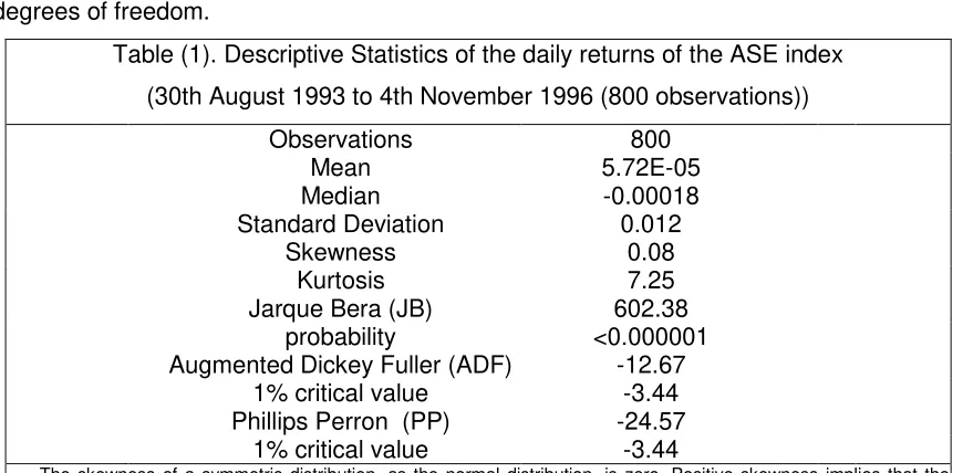
. The data set covers the period from August 30th, 1993 to November 4th, 1996, a total of 800 trading days. Table 1 presents the descriptive statistics. For an estimated kurtosis equal to 7.25 and an estimated skewness equal to 0.08, the distribution of returns is flat (platykurtic) and has a long right tail relative to the normal distribution. The Jarque Bera (JB) statistic (Jarque and Bera (1980)) is used to test whether the series is normally distributed. The test statistic measures the difference of the skewness and kurtosis of the series from those of the normal distribution. The JB statistic is computed as:











2

_

_

3

2

4



6



T

S

K

JB

, (5.1)

where T is the number of observations,

S

is the skewness and K is the kurtosis. Under the null hypothesis of a normal distribution, the JB statistic is



2 distributed with 2 degrees of freedom.

Table (1). Descriptive Statistics of the daily returns of the ASE index (30th August 1993 to 4th November 1996 (800 observations))

Observations 800

Mean 5.72E-05

Median -0.00018

Standard Deviation 0.012

Skewness 0.08

Kurtosis 7.25

Jarque Bera (JB) 602.38 probability <0.000001 Augmented Dickey Fuller (ADF) -12.67

1% critical value -3.44 Phillips Perron (PP) -24.57

1% critical value -3.44

The skewness of a symmetric distribution, as the normal distribution, is zero. Positive skewness implies that the distribution has a long right tail. Negative skewness implies a long left tail distribution.

The kurtosis of the normal distribution is 3. If the kurtosis exceeds 3, the distribution is peaked (leptokurtic) relative to the normal. If the kurtosis is less than 3, the distribution is flat (platykurtic) relative to the normal.

Under the null hypothesis of a normal distribution, the JB statistic is χ2

distributed with 2 degrees of freedom. The reported probability is the probability that the JB statistic exceeds, in absolute value, the observed value under the null hypothesis.

ADF: The null hypothesis of non-stationarity is rejected if the ADF value is less than the critical value. (4 lagged differences).

[image:15.612.90.525.394.608.2]

From Table 1, the value of the JB statistic obtained is 602.38 with a very low p-value (practically zero). So, the null hypothesis of normality is rejected. In order to determine

whether

 

y_t is a stationary process, the Augmented Dickey Fuller test (ADF) (Dickey and Fuller (1979)) and the nonparametric Phillips Perron (PP) test (Phillips (1987), Phillips and Perron (1988)) are conducted.

The ADF test examines the null hypothesis, H0 :



0, versus the alternative,

0

:

1





H

, in the following regression:

t i

i t i t

t c y y

y









  

 





 



1

1 , (5.2)

where  denotes the difference operator. According to the ADF test, the null hypothesis of non-stationarity is rejected at the 1% level of significance for any lag order up to

12





. The test regression for the PP test is the AR(1) process:

t t

t c y

y  







 1 . (5.3)

While the ADF test corrects for higher order serial correlation by adding lagged differenced terms on the right hand side, the PP test makes a correction to the t statistic of

the



coefficient from the AR(1) regression to account for the serial correlation in



t. The

correction is nonparametric since an estimate of the spectrum of



_t at frequency zero,

that is robust to heteroscedasticity and autocorrelation of unknown form, is used. According to the PP test, the null hypothesis is also rejected at the 1% level of significance.

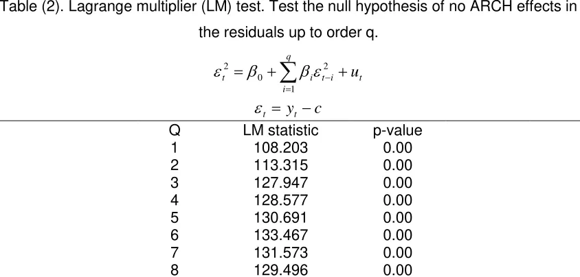
Table (2). Lagrange multiplier (LM) test. Test the null hypothesis of no ARCH effects in the residuals up to order q.

c y

u

t t

t q

i

i t i t

 

 





 











1 2 0

2

Q LM statistic p-value

1 108.203 0.00

2 113.315 0.00

3 127.947 0.00

4 128.577 0.00

5 130.691 0.00

6 133.467 0.00

7 131.573 0.00

8 129.496 0.00

[image:16.612.96.518.489.691.2]

The most commonly used test, for examining the null hypothesis of homoscedasticity against the alternative hypothesis of heteroscedasticity, is Engle’s (1982) Lagrange multiplier (LM) test. The ARCH LM test statistic is computed from an auxiliary test regression. To test the null hypothesis of no ARCH effects up to order q in the residuals, the regression model

t q

i

i t i

t  



u

1 

2 0

2









, (5.4)

with



_t  y_t c is run. Engle’s test statistic is computed as the product of the number of observations times the value of the coefficient of variation R2 of the auxiliary test regression. From Table 2, the values of the LM test statistic for

q



1

,...,

8

are highly significant at any reasonable level.

As, according to the results of the above tests, the assumptions of stationarity and

ARCH effects seem to be plausible for the process

 

yt of daily returns, several ARCH

models are considered in the sequel. It is assumed, specifically, that the conditional mean

is considered as a



th order autoregressive process as defined in (2.2) and the

conditional variance



_t2 is assumed to be related to lagged values of



t and



t

according to a GARCH(p,q) model, an EGARCH(p,q) model or a TARCH(p,q) model as defined by (2.4), (2.6) and (2.7), respectively. Thus, the AR(



)GARCH( p,q), AR(



)EGARCH(p,q) and AR(



)TARCH(p,q) models3 are applied, for





0

,...,

4

,

2

,

1

,

0



p

and

q



1

,

2

, yielding a total of 90 cases.

Since, in estimating non-linear models, no closed form expressions are obtainable for the parameter estimators, an iterative method has to be employed. The value of the

parameter vector



that maximizes lt

 



, the log likelihood contribution for each

observation

t

, is to be found. Iterative optimization algorithms work by starting with an initial set of values for the parameter vector



, say



 0 , and obtaining a set of parameter values



 1 , which corresponds to a higher value of lt

 



. This process is repeated until

the objective function l_t

 



no longer improves between iterations. In the sequel, the Marquardt algorithm (Marquardt (1963)) is used. This algorithm modifies the Berndt, Hall,

Hall and Hausman, or BHHH, algorithm (Berndt et al. (1974)) by adding a correction matrix to the Hessian approximation (i.e., to the sum of the outer product of the gradient vectors for each observation’s contribution to the objective function). The Marquardt updating algorithm is computed as:

   

_

   

_

 

 

 

































T

t i t T

t

i t i t i

i

l

aI

l

l

1 1

1 1











, (5.5)

where I is the identity matrix and a is a positive number chosen by the algorithm. The effect of this modification is to push the parameter estimates in the direction of the gradient vector. The idea is that when we are far from the maximum, the local quadratic approximation to the function may be a poor guide to its overall shape, so it may be better off to simply follow the gradient. The correction may provide a better performance at locations far from the optimum, and allows for computation of the direction vector in cases where the Hessian is near singular.

The quasi-maximum likelihood estimator (QMLE) is used, as according to Bollerslev and Wooldridge (1992), it is generally consistent, has a limiting normal distribution and provides asymptotic standard errors that are valid under non-normality.

In order to compute the sum of squared standardized one step ahead prediction errors, a rolling sample of constant size equal to 500 is used, or

T



500

, so 300 one step ahead daily forecasts are estimated. The out-of-sample data set is split into 5 subperiods and the SPEC model selection algorithm is applied in each subperiod separately. Thus, the model selection is revised every 60 trading days and the information set includes daily continuously compound returns of the two most recently years, or 500 trading days. The choice of a 60-day length for each subperiod is arbitrary. The sum of the squared one step

ahead prediction errors,



T_t_Ts_1

 

ztt_

2 1 |

ˆ , is estimated for each model and presented in Table

3, in the Appendix. The models selected for each subperiod and their sums of the squared standardized one step ahead prediction errors are:

Subperiod Model Selected





__

 





s

T

T

t 1 ztt

2 1 |

ˆ

min

[image:19.612.102.506.149.365.2]

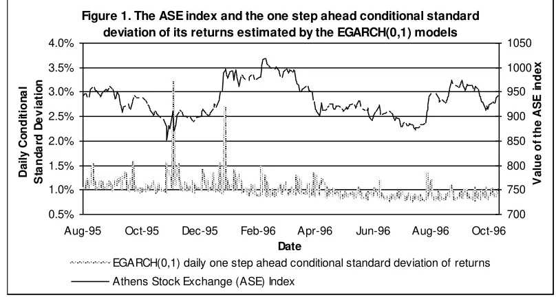
According to the SPEC selection method, the exponential GARCH(0,1) model describes best the conditional variance for the total examined period of 300 trading days. It is selected by the SPEC selection method in each subperiod. Figure 1 shows the daily value of the ASE index and the one step ahead conditional standard deviation of its returns.

Figure 1. The ASE index and the one step ahead conditional standard deviation of its returns estimated by the EGARCH(0,1) models

0.5% 1.0% 1.5% 2.0% 2.5% 3.0% 3.5% 4.0%

Aug-95 Oct-95 Dec-95 Feb-96 Apr-96 Jun-96 Aug-96 Oct-96

Date

D

a

il

y

C

o

n

d

it

io

n

a

l

S

ta

n

d

a

rd

D

e

v

ia

ti

o

n

700 750 800 850 900 950 1000 1050

V

a

lu

e

o

f

th

e

A

S

E

in

d

e

x

EGARCH(0,1) daily one step ahead conditional standard deviation of returns Athens Stock Exchange (ASE) Index

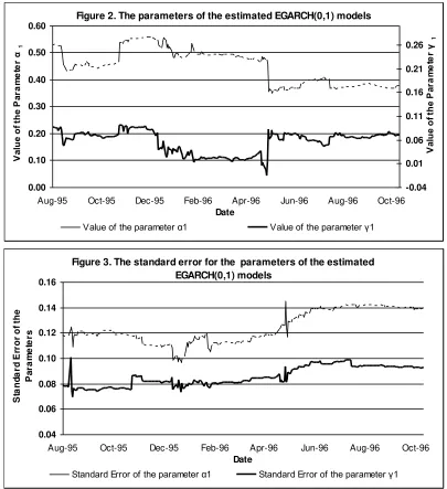
Despite the fact that an asymmetric model is selected by the SPEC algorithm, there are no asymmetries in the ASE index volatility. According to Figure 1, the major episodes of high volatility are not associated with market changes of the same sign. Figure 2 presents

the values of the parameters

a

₁ and



₁ of the 300 estimated EGARCH(0,1) models, while Figure 3 depicts the relevant standard errors for the parameters

a

₁ and



₁. Obviously, the

1



parameter, which allows for the asymmetric effect, is positive but statistically

insignificant. Therefore, the asymmetric relation between returns and changes in volatility does not characterize the examined period.

An interesting point is that the higher order of the conditional mean autoregressive process is chosen as adequate to produce more accurate predictions for the first and the fourth subperiods. As concerns the first subperiod, the AR(2)EGARCH(0,1) model

t t t

t c c y c y

y  ₀  _{1 1} _{2 2} 



 

_

















 

 

1 1 1 1 1 1 0 2

ln

t t

t t

t

a

a

_











,

(5.6)

is the one with the lowest value of



560_

 

_

501 2

1 |

ˆ

t ztt equal to 21.961. The hypothesis:

is tested versus

H1: The model AR(2)EGARCH(0,1) produces “better” predictions than modelX ,

[image:20.612.103.508.128.571.2]

with X denoting any one of the remainder models.

Figure 2. The parameters of the estimated EGARCH(0,1) models

0.00 0.10 0.20 0.30 0.40 0.50 0.60

Aug-95 Oct-95 Dec-95 Feb-96 Apr-96 Jun-96 Aug-96 Oct-96

Date

V

al

ue

o

f t

he

P

ar

am

et

er

α

1

-0.04 0.01 0.06 0.11 0.16 0.21 0.26

V

al

ue

o

f t

he

P

ar

am

et

er

γ

1

Value of the parameter α1 Value of the parameter γ1

Figure 3. The standard error for the parameters of the estimated EGARCH(0,1) models

0.04 0.06 0.08 0.10 0.12 0.14 0.16

Aug-95 Oct-95 Dec-95 Feb-96 Apr-96 Jun-96 Aug-96 Oct-96

Date

S

ta

n

d

a

rd

E

rr

o

r

o

f

th

e

P

a

ra

m

e

te

rs

Standard Error of the parameter α1 Standard Error of the parameter γ1

Note that the correlation between the standardized one step ahead prediction errors is

greater than 0.9 in each case. If 









560_  _

501 2 1 | 1

), 1 , 0 ( ) 2 (

60 21.96 _t ˆ

X t t X

EGARCH AR

z Z



k

a



CGR



30

,



0

.

9

,





, the null hypothesis of equivalent predictive ability of the models

Figure 4, in the Appendix, depicts the one step ahead 95 per cent prediction

intervals for the models with the lowest



T_t_Ts_1

 

ztt_

2 1 |

ˆ in each subperiod. The prediction

intervals are constructed as the expected rate of return plus\minus 1.96 times the

conditional standard deviation, both measurable to

t



1

information set:



ˆ

t_|t₁



1

.

96



ˆ

t_|t₁.

So, each time next day’s prediction interval is plotted, only information available at current day is used. Remark that around November 1995, a volatile period, the prediction interval in Figure 4 tracked the movement of the returns quite closely (seven outliers, or 2.33%, were observed).

6 . A n A l t e r n a t i v e A p p r o a c h

In this section an in-sample analysis is performed in order to select the appropriate models describing the data. Then, the selected models are used to estimate the one step

ahead forecasts. Having assumed that the conditional mean of the returns follows a



th order autoregressive process, as in (2.2), Richardson and Smith (1994) developed a test for autocorrelation. It is a robust version of the standard Box Pierce (Box and Pierce

(1970)) procedure. For pi denoting the estimated autocorrelation between the returns at

time

t

and ti, the test is formulated as:

 

_







r

i i

i

c

p

T

r

RS

1 2

1

, (6.1)

where T is the sample size and c_i is the adjustment factor for heteroscedasticity, which is calculated as:





 

2 2 2

,

t i t t i

y Var

y y Cov

c   , _(6.2)

where yt  yt T



T_t1yt

1

. Under the null hypothesis of no autocorrelation, the statistic is

asymptotically distributed as



2 with r degrees of freedom. If the null hypothesis of no autocorrelation cannot be rejected, then the returns’ process is equal to a constant plus the residuals,



_t. In other words,

 

y_t follows the AR(0) process. If the null of no autocorrelation is rejected, then

 

yt follows the AR(1) process. In order to test for the

asymptotically distributed as



2 with r1 degrees of freedom. The test is calculated on 7 autocorrelations



r



7



for 800 observations yielding a value equal to

 

2

05 . 0 , 7

86 , 14

7  



RS . As the null hypothesis of no autocorrelation is rejected the test is run on the estimated residuals from the AR(1) model that gives RS

 

6 12,33



₆2 _,0.05. Thus, a first order autocorrelation is detected for the returns’ process. Note that the AR(1) form allows for the autocorrelation imposed by discontinuous trading.

Having defined the conditional mean equation, the next step is the estimation of the conditional variance function. The AIC and the SBC criteria are used to select the appropriate conditional variance equation. Note that the AIC mainly chooses as best the less parsimonious model. Also, under certain regularity conditions, the SBC is consistent, in the sense that for large samples it leads to the correct model choice, assuming the “true” model does belong to the set of models examined. Thus, the SBC may be preferable to use. As concerns the specific dataset, both the AIC and SBC select the GARCH(1,1) model as the most appropriate function to describe the conditional variance. So, performing an in-sample analysis the AR(1)GARCH(1,1) model is regarded as the most suitable, which is the model applied in most researches. Figure 5, in the Appendix, presents the in-sample 95 per cent confidence interval for the AR(1)GARCH(1,1) model. There are fourteen observations, or 4.66%, outside the confidence interval.

In order to compare the model selection methods, the choice of the models should be conducted at the same time points. Thus, the Richardson Smith test for autocorrelation detection and the information criteria for model selection are used in each subperiod separately. The models selected for in each subperiod are:

Subperiod Richardson Smith Model selection

SBC Model Selection

AIC Model Selection

1. AR(3) GARCH(1,1) EGARCH(1,2)

2. AR(2) GARCH(2,1) GARCH(2,1)

3. AR(0) GARCH(1,1) GARCH(1,1)

4. AR(0) GARCH(1,1) GARCH(1,1)

5. AR(0) GARCH(1,1) TARCH(1,1)

Based on Table 4, the hypothesis that the model selected by the in-sample analysis is

equivalent to the model with minimum value of



T_s_

 

_

T

t 1 ztt

2 1 |

ˆ is rejected in the majority of

the cases.