G CSF Reduction: The Equilibrium Solution for the DDE and a Sufficient Condition for the Global Stability

G-CSF Reduction: The Equilibrium Solution for the DDE

and a Sufficient Condition for the Global Stability

S.Balamuralitharan

Department of Mathematics,

Sri Ramanujar Engineering College, Vandalur Chennai 600 048, INDIA

S.Rajasekaran

Department of Mathematics, B.S. Abdur Rahman University, Vandalur

Chennai 600 048, INDIA

ABSTRACT

In this paper, we introduce delay differential equation (DDE) models of the hematopoietic system designed for the study of the effects of Granulocyte-Colony Stimulating Factor (G-CSF) administration. G-CSF is used clinically for treating subjects presenting low numbers of white blood cells, a condition referred to as Neutropenia that can result from different causes. The aim of this paper is to study alternative treatment that would minimize the use of G-CSF drug using a mathematical modeling. We propose is a parameter estimation model that considers G-CSF administration for Cyclical Neutropenia (CN), a dynamical disorder characterized by oscillations in the circulating neutrophil count. The model develops the dynamics of circulating blood cells before and after the G-CSF treatment. The model develops the equilibrium solution for the DDE and a sufficient condition for the global stability. The model focuses on the effects of two compartments forms of G-CSF for the treatment of CN (Fast Fourier Transform simulations). For each model, we use a combination of mathematical analysis and numerical simulations (linear chain trick) to study alternative G-CSF treatment that would be efficient while reducing the amount of drug. This reduces the quantity of G-CSF required for potential maintenance. This model gives us good result in treatment. The changes would be analytical and reduce the risk side as well as the cost of treatment in G-CSF.

Key words

: CN, G-CSF, FFT Simulation, DDE, Global Stability.

1.

INTRODUCTION

We are also interested in studying the effects of G-CSF reduction, but for neutropenia. Granulocyte-colony stimulating factor (G-CSF) stimulates neutrophils production and is used analytically for treating neutropenia (low neutrophil levels). We used a mathematical modeling approach and analytical to study alternative G-CSF treatment regimens for cyclical neutropenia. We found that G-CSF can either increase the amplitude of the oscillations. These results suggest that administration of G-CSF can affect the dynamical behavior of the granulopoiesis system (Figure 1 and 2 gives general information). Indeed, G-CSF is widely used in oncological practice for treating neutropenia and preventing infections that often follow G-CSF treatment. To better study this situation, we develop a delay differential equation model for the regulation of neutrophil production. We use explicit functions for modeling the effects of G-CSF on the amplification factor, the post mitotic transit time and the apoptosis rates. Using a combination of analysis and numerical simulations, we use this model to study the effects of delaying G-CSF treatment following for two recombinant forms of G-CSF (Tissue G-CSF and Circulating G-CSF). We

[image:1.595.318.537.254.636.2]

also examine the consequences of varying the duration of G-CSF drug reduction and study some dynamical properties of the system.

[image:1.595.318.538.257.432.2]

Fig 1: G-CSF drug Neupogen & EPO (Image: Google Images)

Fig 2: G-CSF Transcription model for cell differentiation (Image: Google Images)

It is very important to note that the estimates of '

r

P all satisfy the global stability condition of Pr' D as given in eqn. (21).

value, there is quite a difference between the other preliminary parameter estimates and the actual values that were arrived at in the fit. The origin of this discrepancy is primarily due to the fact that the actual value of  as given ranges from about 2 to 5, values well below the previously estimated values of 8-16. Though we have no data that would allow us to estimate the value of  in normal dogs, if they have hematopoietic systems similar to humans and the mouse, the low values of  calculated here would suggest that the ANC (Absolute Neutophil Count) has much less available in their neutrophil control system to respond to increased demands for neutrophils. This decreased elasticity in the ANC translates to between two and three fewer potential divisions within the neutrophil production system [5-10].

This suggests that in the Neutrophil there is not only an alteration within the stem cell compartment giving rise to the oscillatory dynamics, but that there is also a significant depression of the efflux from the stem cell population into the recognizable neutrophil line. Taken together with the low values of, we tentatively conclude that cyclical neutropenia is a hematopoietic defect in which there is abnormal cell loss within the stem cell compartment that is also expressed in the progeny committed to the production of neutrophils. This same point has been emphasized analytically who showed that normal CN and induced CN had the same number of G-CSF receptors on neutrophil precursors, and that the binding constant of G-CSF with the receptor was unaltered between the two. They further found that we required a seven fold higher concentration of G-CSF to achieve half maximal colony growth compared to normal CN, and concluded that the defect in cyclical neutropenia is due to a defect in the signal transduction pathway distal to G-CSF receptor binding [2, 4, 5, 10-12]. Within the context of the model that we have presented and analyzed, we provisionally interpret this analytical finding to imply that the values of G-CSF injection tabulated are of the order of seven parameters the values that will be found in ANC.

2. BACKGROUND ON

MATHEMATICAL THEOREM

Suppose that Pr is a continuous and decreasing function.

Assume that xs is the unique root of the equation f 2

(s) = s in the interval [0, ) . Let : (,0][0, ) be a bounded

function and x (t) be the solution of    r

dx

Dx P x dt

satisfying the initial condition x t( )( )t for t ( ,0]. Then x(t) converges to xs as t .

Proof: First, observe that any solution '( )x t is a bounded and

nonnegative function. Since 0P x_r( )P_r(0) a solution '( )

x t satisfies the inequalities

( ) '( ) ( ) (0), 0.

Dx t x t  Dx t Pr t

As x(0)



0 from the first inequality it follows that x(t)



0 and the second inequality implies that x(t) is a bounded function. Now we check that if

0 liminf ( ) limsup ( )

 

     

t t

A x t x t B (1)

then

1 ( ) liminf ( ) limsup ( ) 1 ( )

 

 r    r

t t

P B x t x t P A

D D (2)

Fix 0. Then there exists t0> 0 such that

A  x t( ) B ,tt0 (3)

0

0

( ) ( ) ( ) ( ) ( ) ,

 





_

 

_

  

m

t t

m

M t t

x t x t u g u du x t u g u du t t M

0

0

( ) ( ) ( )  ( ) ,

 



 

_



_

m

t t

M t t

x t B g u du g u du (4) where sup



x t( ) :tR



. Since g is a density there exists t1>t0+Mm such that

0

( ) 









t t

g s ds fortt₁ . Consequently,

1

( )   , 

x t B t t

Since Pr is a decreasing function we have

1 ( ) (   ), 

r r

P x t P B t t

This leads to the following differential inequality: 1

'( ) ( ) r( ),

x t  Dx t P B   tt Let y(t) be the solution of the equation

y t'( ) Dy t( )P Br(   ) (5)

with the initial condition x(t1) = y(t1). Then x(t)



y(t) for

t



t1. Since the constant solution 0

( )

r

P B y

D

   

 of eqn.

(5) is asymptotically stable we have lim ( ) ₀

ty t y . The

inequality x(t)



y(t) implies that

( )

liminf ( ) r t

P B x t

D

  

 

 (6)

Let 0. Then from eqn. (6) we get ( ) liminf ( ) r t

P B x t

D

 

In a similar way, we obtain

( ) limsup ( ) r t

P A x t

D

 

Since the solution x t'( ) is a bounded function there exist constant A and B such that 0 A xsB A, x t( )B t, R. From eqns. (1) and (2) it follows that:

2 2

( ) liminf ( ) limsup ( ) ( )

n n

t t

f A x t x t f B

 

   (7)

for n = 1, 2,…. Since f is a decreasing function, the function f 2 is increasing [6 - 9]. The assumption that xs is the unique

fixed point of the function f 2 in the interval [0, ) implies that

2 2

( ) s, s ( ) , s

xf x x x f x x xx

Hence, 2 2

lim n( ) ,lim n( )

s s

tf A x tf B x and we finally obtain

that

lim ( ) _s

tx t x

This completes the proof.

2.1 MODEL DEVELOPMENT

Let the density of white blood cells in the circulation be x(t) (units of cells mm-3 blood), D the random disappearance rate of circulating white blood cells (days-1), and Pr the production

rate (cells mm-3 day-1) of white blood cell precursors in the bone marrow [13 – 19]. We assumed that the rate of change of the circulating white blood cell density is made up of a balance between the loss of white blood cells (-Dx) and their production (P x_r ), so

r

dx

Dx P x

where in ( )x t is x(t-M) weighted by a distribution of maturation delays. x t( )is given explicitly by

( ) ( ) ( ) ( ) ( )

m

m

t M

M

x t x t u g u du x u g t u du

 





_

 

_

 (9)

Mm is the minimal maturation delay and g(M) is the density of

the distribution of maturation delays as specified below. Since g(M) is a density,

0

( ) 1

g u du







(10) To completely specify the semi-dynamical system described by eqns. (8) and (9) we must additionally give an initial function

x t( ')( '), 't t ( ,0) (11) ,

( ) 0,M Mm ( )

g M   g M

1

( )

0, ,

( ) ,

( ( )

1 (

)

) m

m

m

a M M m

m m

M M

a

M M e M M

g M g M

m



  

 

 





(12)

with a, m > 0, was able to give an excellent fit to the existing data on neutrophil maturation times. The parameters m, a, and Mm in the density of the gamma distribution can be related to

certain easily determined statistical quantities. Thus, the average of the up shifted density is given by

2

0

1

( ) m

M Mg M dM

a

 _



_



(13)

so the average maturation delay is

2

1

m m

m

M M M M

a



   

(14) and the variance is

2

2 1 m

a

  

(15) Using eqns. (13) and (15) the gamma distribution parameters m and a are

2

2 2

2, 2 1

M M

a m

 

  

To write out the explicit form for the output flux P x tr( , ) , the following considerations are important. It is assumed that the maximal amplification (Am) of cells entering the recognizable

neutrophil precursor pool is modified by apoptosis at a rate



that is under the control of the number of circulating neutrophils xM so  ( )x . The maximal amplification is

thereby modified to becomeAmexp(( )x M), and if the input flux into the recognizable compartment of neutrophil precursors is Pi (t) then the efflux corresponding to the cells with transit time M is

( )

( , ) x M

r i m

P x M P A e . (16) To take into account the distribution of transit times we must integrate over the entire range of available transit times to give the final form for

1 ( )

( ) ( , ) ( )

( )

m

m

m

x M

r r i m

M

a

P x P x M g M dM P A e

a x



  

  

   



 



(17)

In keeping with the known inverse relation between apoptosis and the levels of circulating G-CSF and the inverse relation between circulating G-CSF levels and the peripheral neutrophil count, we have taken a form for  given by

( ) m

x x

x

 

 



(18)

So Pr will be a monotone decreasing function of x . Thus, the

control of neutrophil production has the characteristics of a negative feedback system with distributed delay. The constants _m (the maximum rate of apoptosis) and  (the value of x at which apoptosis reaches half maximal values) in eqn. (18) will be estimated [20].

3. TESTING MATHEMATICAL

ANALYSIS

The equilibrium solution for the functional differential equations (8) and (9) occurs when

0 r( )

dx

Dx P x

dt  

(19)

so the steady state xs is defined implicitly by the solution of

the equation

DxsP xr sPrs (20)

Given the monotone decreasing nature of the negative feedback production rate P xr( ) inferred from the biology, there can be but a single unique value for the steady-state white blood cell density xs. The value of PrsDxs is

equivalent to the Granulocyte Turnover Rate (GTR). Let ( ) P xr( )

f x D

 . Then xs is the unique root of the equation f

(s) = s in the interval [0, ) . Let 2

f  f f. Then xs is also a

root of the equation f 2(s) = s. Now we give a sufficient condition for the global asymptotic stability.

If '

r

P D, then f'1 and xs is the unique root of

f 2(s) = s. However, if the function Pr is of the form (17) then

both analytic and numerical results indicates that xs is the

unique root of f 2(s) = s if and only if '

r

P D . Thus, a sufficient condition for the global stability of xs is

'

rs

P D

(21) To develop the theoretical background for preliminary parameter estimates, we consider the response of this system to a periodic cellular influx coming from the hematopoietic stem cell compartment when we are near to a steady state [3, 13]. Throughout this analysis, an important parameter that will appear is the slope of the production function Pr evaluated at the steady state, denoted by

'

r

P . Because of our arguments concerning the negative feedback nature of the peripheral control mechanisms acting on neutrophil production, we know that this slope must be non-positive. To examine the response to a periodic input, we assume that the production of neutrophils can be written in the form

P x tr( , )P A xi ( ) (22)

where A x( ) is the amplification within the neutrophil precursor compartment, and

( ) (1 ( ) ), [0,1]

i wt

i is

P t P I w e 

(23) is the assumed oscillating hematopoietic stem cell influx with mean value Pis , amplitudePisRe( ( ))I w , and period

2 w



. The term

( ) ( )

m

i wM i wM

M

a

I w e g M dM e

iw a



  

 _{  }



 



accounts for the distribution of maturation times. With these assumptions, we can write out eqn. (8) for small deviations of x from xs. In the first approximation this gives

' '

( ) ( ) i wt( ( ) )

rs s rs rs s rs

dx

Dx P x x P I w e P x x P

dt        

(25)

PrsP xr s (26)

' ( ) , r rs s P x

P x x

x     (27)

Utilizing eqn. (20) and defining the deviation from equilibrium as z(t) = x(t) - xs, we can rewrite Eqn. (25) in the

form

' '

( ) i wt( )

rs rs rs

dz

Dz P I w e P P

dt   

(28)

Table 1. The results of fitting the 7 parameter model

w

P a0 a1 a2 a3 a4 a5 a6

0.465 13.5 1.06 0.99 0.09 0.008 0.0001 0.00004 0

0.470 13.4 1.80 1.47 0.70 0.08 0.006 0.0005 0

0.464 13.5 2.44 2.15 1.54 0.9 0.08 0.004 0

0.500 12.6 2.89 2.69 0.58 0.03 0.007 0.0002 0

0.426 14.7 4.49 2.94 2.12 1.23 0.98 0.08 0

0.438 14.3 5.79 5.05 3.60 2.56 1.43 0.87 0.1

[image:4.595.59.275.471.755.2]

0.418 15.0 6.26 6.04 5.95 4.2 3.7 2.01 0.9

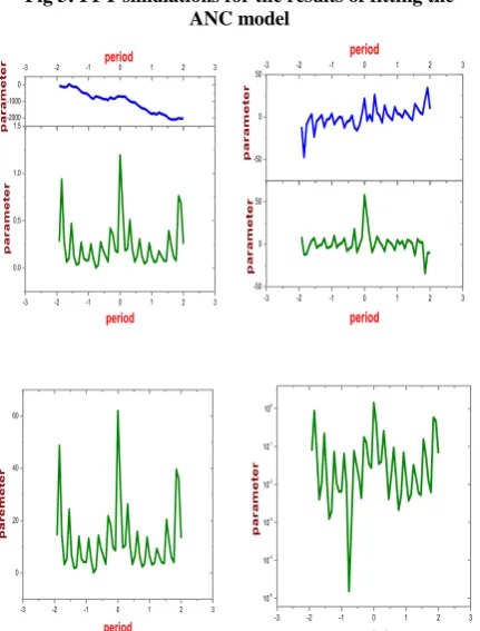
Fig 3: FFT simulations for the results of fitting the ANC model

To use the existence of the first, second, and sometimes third-harmonic components evident in the FFT simulation and reflected in the fits of eqn. (28), we assume that the deviation z of the circulating neutrophil numbers from their steady-state value can be expanded in the series representation

0

( ) ( )ik wt

k k

z t c w e









(29)

Substituting eqn. (29) into eqn. (28) and equating the coefficients of the terms exp(ik wt) for k= 0, 1, …,6 yields

' 0( rs)

c DP as expected, so c0 = 0,

1 ' ( ) ( ) ( ) rs rs

P I w c w

D iw P I w

    (30) ' 2

2 1 '

[ ( )]

( ) ( )

2 (2 )

rs

rs

P I w

c w c w

D iw P I w

 

 

(31)

In the general case, the relation is

' 1 ' 0 ( ) ( ) ( ) ( ) ( ) ( ) rs k k ik wt k rs k

P I w I k w

c w c w

D c w e P I k w

     



 (32)

From the above considerations, in the neighborhood of the steady state we can write

0

( ) Re[ ( )] Re ( )ik wt

s s k

k

x t x z t x c w e

        _{ } 



 (33)

We took all of the ANC of the seven parameters and did a FFT (Fast Fourier Transform) fit to the equation

6 6

0 0

1 1

( ) cos( ) Re(ik wt pk)

k k k

k k

x t a a k wt p a a e 

 

 



  



(34)

The values of the constants w, a0, a1,…, a6 resulting from

these determinations are given in Table1. The value of a0

gives the average value of the circulating neutrophil number over several cycles in a given CN (see Figure 3). If we write the coefficients c wk( ) in polar form

arg( ( ))

( ) ( ) i ckwk

k k

c w c w e

(35) then we can identify a0 = xs and

( ) , 0,1,...,6.

k k

a c w k

(36)

3.1

PARAMETER ESTIMATION

The easiest parameter to estimate is D. Labeled neutrophils disappear from the circulation with a half-life t1/2 of about 7 hr

in both normal CN and induced CN with a range of 6.7-7.6 hr. The decay coefficient a of eqn. (8) is related to the t1/2 by

1/ 2 2 In D t  (37)

soD [2.18, 2.48] (days-1). We will take D = 2.3 days-1 corresponding to t1/2 = 7 hr

-1

. To obtain estimates of



and '

rs

P , use eqns. (30) and (31) in eqn. (36) to give

1 ' ( ) ( ) rs rs

P I w a

D iw P I w

    (38) ' 2

2 ' '

( ) [ ( )]

( ) 2 (2 )

rs rs

rs rs

P I w P I w

a

D iw P I w D iw P I w

 

 

   

(39)

All of the quantities in these two equations are known from previous estimates except for , '

rs

P , and the result of solving for these two unknowns are tabulated in Table 2. Similarly we get the other parameters. Two points are noteworthy. First, in every case our analysis indicates that the amplitude of the oscillatory input is close to one indicating that, if the model is

-3 -2 -1 0 1 2 3

0.0 0.5 1.0 1.5 period p a r a m e te r -2000 -1000 0

-3 -2 -1 period 0 1 2 3

p a r a m e te r

-3 -2 -1 0 1 2 3

-50 0 50 period p a r a m e te r -50 0

50-3 -2 -1 0 1 2 3

period p a r a m e te r

-3 -2 -1 0 1 2 3

0 20 40 60 period p a r e m e te r

-3 -2 -1 0 1 2 3

correct, the influx from the stem cell compartment always cycles with a minimum close to zero. Secondly, in every case the values '

rs

P consistent with the data are well above the Hopf bifurcation calculated [14, 15]. This indicates that the neutrophil control loop modeled in this paper would have a locally stable steady state in the absence of any periodic stem cell inputs. This is consistent with the notion that the peripheral control of neutrophil production is not the origin of CN, a conclusion reached and elsewhere based on mathematical modeling. This further supports the idea that the hematopoietic stem cell population may be the source of the oscillations seen in cyclical neutropenia. Finally, two further relations can be derived from the steady state relation (20) that will be of use in estimating the parameters _m and . Namely, at the steady state we have more explicitly

1

s m

m M

s rs is s is s

s

a

Dx P P A P A e

a



 

  

   _{ }



 

(40)

wheres( )xs . Recognize that eqn. (40) can be rewritten in

the form

1

s m

m M

m s

s

A a

e

A a

    

   _{ }

 

(41)

where As is the steady-state amplification. In humans and CN,

it is estimated that  is of the order of 8-16, so with these values we can determine _ssince all of the other parameters are known and tabulated in Table 2. Additionally, at the steady state we have

' ' 1

rs s rs m

s

m

P P M

a





  

    _ 

 

(42)

Given an estimate of the GTR, Prs = xs, eqn. (40) gives an

estimate of the maximum steady state GTRmax = Pis Am

since_s , a, m and Mm are all known. Thus, given an estimate

f _s , eqn. (42) gives a direct estimate of s'and '

r

P has been estimated. To see how this can be used to determine values of the parameters _m and  _{in eqn. (18), note that}

'

2

( )

s m

s

x



 

 



(43)

2 2 '

' , '

s s s

m

s s s s s s

x

x x

 

 

   

 

 

(44)

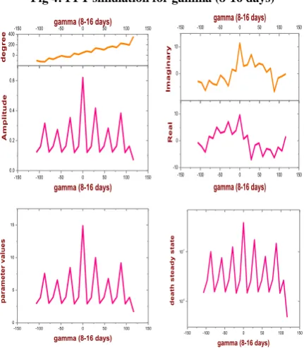
The results of our preliminary parameter estimations for the production rate are contained in Table 2for = 8 and 16 (see Figure 4).

Table 2. Estimates of the parameter

=8 days  _{=16 days}



0.95

0.85 0.93 0.93 0.75 0.95 1.09

'

rs

P

-0.20 -0.91

-1.09 -0.48 -1.2 -1.0 -1.2

s

 0.65 0.65 0.65 0.65 0.65 0.65 0.65

'

s

 0.02 0.06 0.057 0.021 0.035 0.023 0.025

m

 0.68 0.56 0.56 0.56 0.56 0.56 0.56

[image:5.595.320.536.79.326.2]

 0.04 0.28 0.51 0.72 1.73 2.88 3.37

Fig 4: FFT simulation for gamma (8-16 days)

4.

SIMULATION RESULTS

We are now in a position to see if the full nonlinear simulation of our model is capable of reproducing the behavior seen in the CN. The full model as developed above can be written in the form

1 ( )

( )

( )

m

m

x M

i m

dx a

Dx P t A e

dt a x



 

  

    



 

(45)

by combining eqns.(8) and (17), with an assumed periodic input of the form

( ) (1 Re[ ( ) ]), [0,1]

i wt

i is

P t P  I w e 

(46) and x defined by eqn. (9), and ( ) x an ( )I w given by eqns. (18) and (24), respectively. Combining eqns. (45) and (46) we have

1 ( )

(1 Re[ ( ) ]) ( )

m

m

x M i wt

i s m

dx a

Dx P A e I w e

dt a x

 _

 

  

    _   

  (47)

The parameter D is known from the previous section, while a, Mm, and m are given in eqn. (40), and remembering that xs =

a0 from the previous section, we can write

1

0

s m

m

M s

i s m

a

P A Da e

a

    

 _{ }

 

(48)

so given an estimate of _s we have an estimate of the coefficient Pis Am. Further, given an estimate the minimum

values of '

r

P = -1.80 along with _s = 0.25 we can immediately estimate _m= 2.9299 and  ₌ 67.1047 (see Table 3).We have simulated the solution behavior of the full model FFT simulation and fit a polynomial. Selecting values of Pr' ands , we found that we were able to get the closest

fit of the seven data sets using the final parameter values of Table 3, and the results of our numerical simulations (see Figure 5 – 7). In every case, in order to mimic the approach of the ANC numbers to zero at the nadir of each oscillation it was necessary to take =1.

-150 -100 -50 0 50 100 150

0.0 0.2 0.4 0.6

gamma (8-16 days)

A

m

p

li

tu

d

e

0 200

400-150 -100 -50 0 50 100 150

gamma (8-16 days)

d

e

g

r

e

e

-150 -100 -50 0 50 100 150

-10 0 10

gamma (8-16 days)

R

e

a

l

0 10

-150 -100 -50 0 50 100 150

gamma (8-16 days)

Im

a

g

in

a

r

y

-150 -100 -50 0 50 100 150 0

5 10 15

gamma (8-16 days)

p

a

ra

m

e

te

r

v

a

lu

e

s

-150 -100 -50 0 50 100 150 10-2

10-1

gamma (8-16 days)

d

e

a

th

s

te

a

d

y

s

ta

[image:6.595.320.534.75.338.2]

Table 3. Simulation results for the parameters

'

r

P s s' m   P Ais m

data fit _{Eqn. (42) and (44)} (41) and (48)

-0.10 0.2 0.01 0.2 0.07 1.9 4.9

-0.05 0.2 0.03 0.2 0.05 1.9 8.4

-2.00 0.5 0.10 1 2.5 4.9 29

-0.50 0.1 0.02 0.2 5.0 1.3 9.8

-1.50 0.4 0.04 0.7 3.9 3.6 38

-1.70 0.2 0.03 1.8 37 2.2 31

[image:6.595.55.279.92.252.2]

-1.80 0.2 0.03 2.9 67 2.2 34

[image:6.595.72.236.313.505.2]

Fig 5: Polynomial fit for relation between production rate and death rate in two parameters

Fig 6: Polynomial fit for relation between maximum apoptosis rate and apoptosis half maximal values

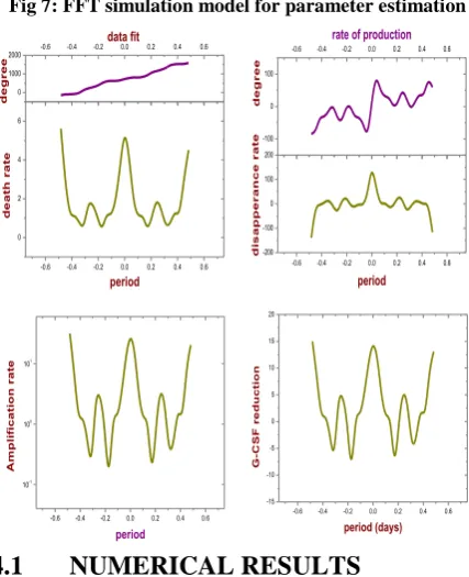
Fig 7: FFT simulation model for parameter estimation

4.1

NUMERICAL RESULTS

We have solved equations numerically using a Runge – Kutta fourth order method (12 iterations) and some parameters values are standard. In the derivation of the model, the loss terms in the equations for c and I do not apply until, respectively (before these times, the loss terms depend on the initial conditions). In solving the problem numerically, it is simplest to accommodate this by taking the loss terms to be zero for these early times, which prevents the possibility of c and I becoming reduce the G-CSF level.

At the standard parameter values of the full solution of

2 (C )C e c c-[ (C) + (K)]C

c c

dC dt

 

 

   

 ,

tends to a stable steady state

C= 0.49999999999999,  = 1,  = 1752, area = 4.4714145457024, K = 41.39276663963,

_c= 0.23272415762423,

c = 0.044785714290213.

Similarly we get the other parameters solutions.

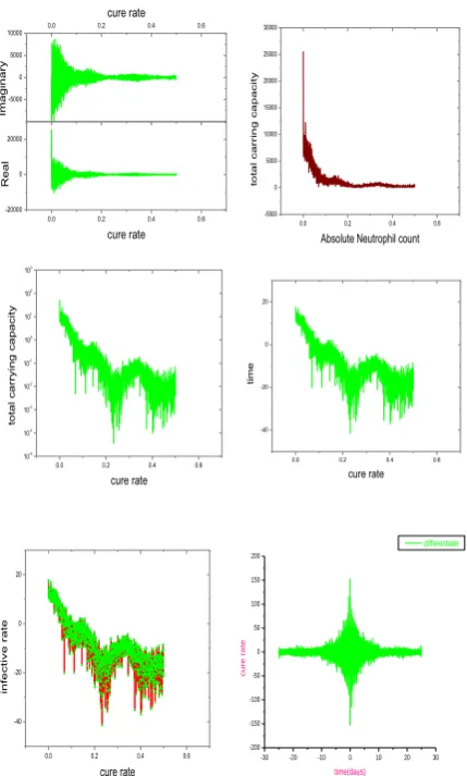
To represent the effect of a disease such as neutropenia, we choose to examine lower values of the parameters c (cure rate) and I (infective rate), and higher values of k (carrying capacity). Analytically with different values of these and other parameters reveals that the model has a confusing variety of behaviors, and many of the features in the simulation of

Figure 8 can be found in the numerical solutions with

differentiate solution. It is noteworthy in the solutions that neutrophil oscillations tend to be irregular for an initial transient period of some 30 days. This is such a long period that it is reasonable to suppose that external physiological influences will cause the dynamics to remain in a transient state. This will not be revealed in the eventual oscillatory solutions we obtain, since no injection of long time secular influences is included. This figure shows the behavior we have described. The neutrophil population tracks the long period oscillation of the stem cells, and a higher frequency oscillation is excited at the peak of the oscillations.

0 1 2 3

0 30 60

a

p

o

to

s

is

h

a

lf

m

a

x

im

a

l

v

a

lu

e

s

maximum rate of apotosis

apotosis half maximal values

maximum rate of apotosis

-0.6 -0.4 -0.2 0.0 0.2 0.4 0.6 0

2 4 6

period

d

e

a

th

r

a

te

0 1000

2000 -0.6 -0.4 -0.2 0.0 0.2 0.4 0.6 data fit

d

e

g

re

e

-0.6 -0.4 -0.2 0.0 0.2 0.4 0.6 -200

-100 0 100 200

period

d

is

a

p

p

e

r

a

n

c

e

r

a

te-100

0 100

-0.6 -0.4 -0.2 0.0 0.2 0.4 0.6

rate of production

d

e

g

r

e

e

-0.6 -0.4 -0.2 0.0 0.2 0.4 0.6 10-1

100 101

period

A

m

p

li

fi

c

a

ti

o

n

r

a

te

-0.6 -0.4 -0.2 0.0 0.2 0.4 0.6 -15

-10 -5 0 5 10 15 20

period (days)

G

-C

S

F

r

e

d

u

c

ti

o

[image:6.595.82.255.571.726.2]

[image:7.595.59.274.95.452.2]

Fig 8: Numerical results of four parameters in FFT simulation

-30 -20 -10 0 10 20 30 -200

-150 -100 -50 0 50 100 150 200

cu

re

rate

time(days)

differentiate

4.2

G-CSF DRUG LEVEL REDUCTION

G-CSF is a hematopoietic growth factor that stimulates the bone marrow to increase the production of neutrophils. Thus, this is the treatment of choice for neutropenia. It is produced naturally in the body, but recombinant forms of G-CSF (Neupogen, lenograstim and Neulasta) are used as drugs to accelerate recovery from neutropenia (see Table 4). In this study, we will only consider the reduction of drug. Another drug is the same molecule as G-CSF drug but to which a 20 kDa polyethylene glycol moiety has been added. This addition changes its pharmacokinetic properties and virtually eliminates renal clearance.

Other than a difference in their clearance rate, both molecules have the same effects: they boost the number of neutrophils by decreasing the apoptosis rates in neutrophil precursors and thus increasing the effective amplification factor, and accelerating the transit time through the post mitotic pool. We only consider the use of G-CSF following myelosuppressive drug on patients suffering from nonmyeloid types of cancer, e.g. we are assuming that a model of regulation of neutrophil production can be taken to represent a hematological normal individual. Neupogen’s clinical guidance for cancer patients receiving myelosuppressive drug recommends a starting dose of 5 μg/kg/day, subcutaneously. Doses may be increased in increments of 5 μg/kg for each drug cycle, according to the duration and severity of the ANC base (see Figure 9). Neupogen should be administered no earlier than 24 hours after the administration of cytotoxic drug and it should be

administered daily for up to 2 weeks, until the ANC has reached normal levels following the expected induced neutrophil. The recommended dosage of Neulasta is a single subcutaneous injection of 6 mg administered once per drug cycle. Neulasta should not be administered in the period between 14 days before and 24 hours after administration of cytotoxic drug.

Table 4. G-CSF drug level reduced in minimum

C-CSF (x) Max Min ANC (y) Injection=y/x

0.11 2.401 0.753 1.078 9.8

0.1 2.393 0.578 1.031 10.31

0.05 2.342 0.645 0.7515 15.03

0.02 2.300 0.698 0.5234 26.17

0.005 2.260 0.736 0.34555 69.11

0.001 2.237 0.753 0.26014 260.14

0.0001 2.223 0.759 0.2221 2220.9

[image:7.595.312.544.163.483.2]

0.00002 2.220 0.760 0.21476 10738

Fig 9: G-CSF drug level reduced in minimum

5.

RESULTS

There are 4 apoptosis rates to consider (Apoptosis rates_i). Three of them (s,

'

s,mand) vary in response to G-CSF

and circulating G-CSF, whereas we assume that the death rate from the circulating neutrophils s remains unchanged

G-CSF treatment. We take_s= 0.65 (death rate is increased compare to previous studies), '

s=0.02, m=0.68, =0.04,

and '

rs

P = -0.20 (rate of production is reduced). Next, we look at the three other apoptosis rates for cancer subjects, under CN and G-CSF treatment. To simulate non myeloid cancer with the model, we use the same values as for healthy individuals. We take s= 0.20 days

−1

. We estimated '

s to

vary between 0.01 and 0.31 days−1. We take '

s=0.0120

days−1. Finally, we assume that the death rate for the proliferative and non-proliferative precursors are the same (m=0.2136, =0.071). In the normal dog, the steady state

neutrophil production rate (GTR) is about 16.5x108 cells kg-1 day. If indeed, 8 << 16 normally, then we should expect that the maximal normal GTR values are given by 132x108 < PisAm < 264 x10

8

cells kg-1 day. The maximal grey collie GTR

0.0 0.2 0.4 0.6 -20000

0 20000

cure rate

R

eal

-5000 0 5000

10000 0.0 0.2 0.4 0.6

cure rate

Im

agin

ar

y

0.0 0.2 0.4 0.6 -5000

0 5000 10000 15000 20000 25000 30000

Absolute Neutrophil count

tota

l car

ring ca

pacity

0.0 0.2 0.4 0.6 10-5

10-4

10-3

10-2

10-1

100

101

102

103

cure rate

tota

l car

rying ca

pacity

0.0 0.2 0.4 0.6 -40

-20 0 20

cure rate

time

0.0 0.2 0.4 0.6

-40 -20 0 20

cure rate

infect

ive r

ate

0.00 0.05 0.10

0 5000 10000

G

-C

SF

In

je

ct

io

n=y/

x

Circulating C-CSF (x)

[image:7.595.313.544.164.481.2]

values of PisAm = 4.95 tabulated in Table 3 are much less than

one quarter of the minimum of this range [21-23].

6.

CONCLUSION

The simulations shown in[19], using parameters appropriate for the distributions of maturation times, are in good agreement with the result and with the spectral behavior shown in [11]. Further, since the model gives a reasonable representation of the secondary peak on the descending FFT of the neutrophil counts we conclude that this phenomenon is simply due to the nonlinear filtering of a periodic stem cell input by the peripheral neutrophil control system mediated by G-CSF.If this is correct, then we would expect that normally

_m is between about 0.2 and 2.9 day-1. Neupogen’s clinical

guidance for CN patients getting myelosuppressive drug recommends a starting dose of 5 μg/kg/day, subcutaneously. G-CSF injection may be decreased in increments of 5 μg/kg for each drug cycle, according to the duration and severity of the ANC base. Neupogen should be managed no earlier than 12 hours after the administration of cytotoxic drug and it should be directed daily for up to 1 week, until the ANC has reached normal levels of the expected induced neutrophil counting. The suggested dosage of Neulasta is a single hypodermic injection of 6 to 8 mg administered once per drug cycle. Neulasta should not be administered in the period between 12 days before and 24 hours after administration of cytotoxic drug.

7.

REFERENCES

[1] Balamuralitharan S., Rajasekaran S., “A Mathematical Age-Structured Model on Aiha Using Delay Partial Differential Equations”, Australian Journal of Basic and Applied Sciences, Vol. 5, No. 4, pp. 9-15, 2011. [2] Balamuralitharan S., Rajasekaran S., “A Parameter

Estimation Model of G-CSF: Mathematical Model of Cyclical Neutropenia”, American Journal of Computational Mathematics, 2, 12-20, 2012.

[3] Balamuralitharan S., Rajasekaran S., “Analysis of G-CSF Treatment of CN Using Fast Fourier Transform”, Research Journal of Recent Sciences, Vol. 1(4), 14-21, 2012.

[4] Balamuralitharan S., Rajasekaran S., “Stability of the Six Equilibrium States between CN and G-CSF with Infectives Growth Rate Progression: A FFT Study”, ISCA Journal of Biological Sciences, Vol. 1(2), 55-60, 2012.

[5] Basak K and Ozkan O, “Further oscillation criteria for partial difference equations with variable coefficients”, Computers & Mathematics with Applications, Vol. 59, pp. 55–63, 2010.

[6] Changyou W, Shu W, Xiangping Y, and Linrui L, “Oscillation of a class of partial functional population model”, Journal of Mathematical Analysis and Applications, Vol. 368, pp. 32–42, 2010.

[7] Gani T. S and Jehad O. A, “Almost periodic solutions for abstract impulsive differential equations”, Nonlinear Analysis: Theory, Methods & Applications, Vol. 72, pp. 2457–2464, 2010.

[8] Honglian Y and Rong Y, “Global attractor for some partial functional differential equations with finite delay”, Nonlinear Analysis: Theory, Methods & Applications, Vol. 72, pp. 3566–3574, 2010.

[9] Jose M. A, Neus C, and Sergio M. O, “Cascades of Hopf bifurcations from boundary delay”, Journal of Mathematical Analysis and Applications, Vol. 361, pp. 19–37, 2010.

[10] Lianhua H and Anping L, “Existence and uniqueness of solutions for nonlinear impulsive partial differential equations with delay”, Nonlinear Analysis: Real World Applications, Vol. 11, pp. 952–958, 2010.

[11] Pueon P and Meleshko S. V, “Group classification of second-order delay ordinary differential equations”, Communications in Nonlinear Science and Numerical Simulation, Vol. 15, pp. 1444–1453, 2010.

[12] Xiaohua D, Kaining W, and Mingzhu L, “The Euler scheme and its convergence for impulsive delay differential equations”, Applied Mathematics and Computation, Vol. 216, pp. 1566–1570, 2010.

[13] Zhenbin F and Gang L, “Existence results for semi linear differential equations with nonlocal and impulsive conditions”, Journal of Functional Analysis, Vol. 258, pp. 1709–1727, 2010.

[14] Zhenbin F, “Impulsive problems for semi linear differential equations with nonlocal conditions”, Nonlinear Analysis: Theory, Methods & Applications, Vol. 72, pp. 1104–1109, 2010.

[15] Adimy M., and Crauste F., “Global Stability of a Partial Differential Equation with Distributed Delay Due to Cellular Replication”, Nonlinear Analysis: Theory, Methods & Applications, Vol. 54, No. 8, pp. 1469-1491, 2003.

[16] Bélair J., Mackey M.C., and Mahaffy J.M., “Age-Str- uctured and Two-Delay Models for Erythropoiesis”, Mathematical Biosciences, Vol. 128, No. 1-2, pp. 317-346, 1995.

[17] Colijn C., and Mackey M.C., “A Mathematical Model of Hematopoiesis: II. Cyclical Neutropenia”, Journal of Theoretical Biology, Vol. 237, No. 2, pp. 133-146, 2005.

[18] Dale D. C., and Hammond W.P., “Cyclic Neutropenia: A Clinical Review”, Blood Reviews, Vol. 2, No. 3, pp. 178-185, 1988.

[19] Foley C., and Mackey M.C., “Dynamic Hematological Disease: A Review”, Journal of Mathematical Biology, Vol. 58, No. 1-2, pp. 285-322, 2008.

[20] Foley C., Bernard S., and Mackey M.C., “Cost-Effective G-CSF Therapy Strategies for Cyclical Neutropenia: Mathematical Modelling Based Hypotheses”, Journal of Theoretical Biology, Vol. 238, No. 4, pp. 754-763, 2006.

[21] Horwitz M., Benson K.F., Duan Z., Li F.Q., and Person R.E., “Hereditary Neutropenia: Dogs Explain Human Neutrophil Elastase Mutations”, Trends in Molecular Medicine, Vol. 10, No. 4, pp. 163-170, 2004.

[22] Mackey M.C., “Periodic Auto-Immune Hemolytic Anemia: An Induced Dynamical Disease”, Bulletin of Mathematical Biology, Vol. 41, pp. 829-834, 1979. [23] Roeder I., “Quantitative Stem Cell Biology: