Anum Fatima
Department of Statistics
Lahore College for Women University, Lahore, Pakistan [email protected]
Ayesha Roohi
Department of Statistics
Lahore College for Women University, Lahore, Pakistan [email protected]
Abstract
A new mixture of Modified Exponential (ME) and Poisson distribution has been introduced in this paper. Taking the Maximum of Modified Exponential random variable when the sample size follows a zero truncated Poisson distribution we have derived the new distribution, named as Extended Poisson Exponential distribution. This distribution possesses increasing and decreasing failure rates. The Poisson-Exponential, Modified Exponential and Exponential distributions are special cases of this distribution. We have also investigated some mathematical properties of the distribution along with Information entropies and Order statistics of the distribution. The estimation of parameters has been obtained using the Maximum Likelihood Estimation procedure. Finally we have illustrated real data applications of our distribution.
Keywords: Modified Exponential distribution, Information entropies, Maximum Likelihood Estimates, Order Statistics.
1. Introduction
In lifetime data analysis problems the most widely used distribution is exponential distribution. The popularity of the exponential distribution lies in its nice and simple properties. It provides closed form results through simple mechanism in reliability and lifetime testing problems. One property of Exponential distribution is that it supports a constant failure rate. The problem arises in situations when a given data set does not possess a constant failure rate then we cannot use exponential distribution to model the data. Different modifications of the exponential distribution, supporting non-constant failure rates, have been introduced by several authors to handle this problem.
Exponential-Logarithmic (EL) distribution. Mahmoudi and Zakerzadeh (2010) developed the Generalized Poisson-Lindley (GPL) distribution. Barreto-Souza and Bakouch (2010) mixed the Exponential and Lindley distribution to get the Exponential Poisson-Lindley (EPL) distribution. Preda et al. (2011), Hemmati et. al. (2011) and Zakerzadeh and Mahmoudi (2012) obtained the Modified Exponential-Poisson, Weibull-Poisson and Lindley-Geometric (LG) distributions. Bakouch et al. (2012) compounded the Exponentiated Exponential and zero truncated Binomial distributions to get Exponentiated Exponential Binomial (EEB) distribution. Cordeiro and Silva (2014) introduced the Complementary Extended Weibull Power series class of distributions. Mehmoudi and Jafri (2014) also derived a new class of compounded distributions named as Linear Failure Rate-Power series distributions. Asgharzadeh et al. (2014) developed a new family to compound any continuous probability distribution with the Poisson Lindley distribution.
In this paper we have introduced a new probability distribution to model the life time data. In section 2 we have obtained the density function and distribution function of our model along with the survival and hazard rate. In section 3 we have derived several properties of our distribution incuding Quantile function, Characteristic function, Information entropies, Mean deviations and Order statistics. In section 4 we have discussed the Maximum Likelihood Estimates along with the associated large sample inference. In last section we have used three real data sets to illustrate the application of our distribution.
2. Density Function, Distribution Function and Hazard Function
Here we have derived the density function, distribution function survival and hazard functions of the Extended Poisson Exponential distribution.
Marshall and Olkin (1997) introduced a parameterization scheme to get a new family of distributions, given as:
,
1
F y F y a
F y a F y
Using this scheme they have provided a modification of Exponential distribution named as Modified Exponential distribution with distribution function and density function given as:
1
,
1 1
y y
e F y a
a e
2y; , ; y, , 0 1 . 1
y y
a e
f a a and a a
ae
(Marshall & Olkin, 1997)
Let Z be a random variable distributed as Zero truncated Poisson with density function:
,
; , 0. 1 1z
e
P z z
z e
And let Xmax
W1,....,Wz
, then the conditional density of X given Z is:
11
1 ; ,
1
z
x x
z x
a ze e
x f
z a
ae
Hence we get the marginal density of X as:
1
2 1
1
1 ; , ,
!
1 1 1
z x
x z
z
x x
z
e a e
f x a z
z
ae e ae
Making the substitution z 1 v we get the new density function given as:
1 1
2
; , , ; x 0 and , , 0.
1 1
x x
x
e ae x
a e
f x a e a
e ae
(1)
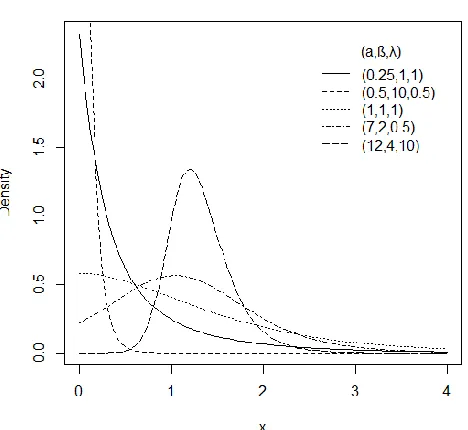
The density given in (1) is named as the “Extended Poisson Exponential (EPE) distribution”.
In the density of Extended Poisson Exponential distribution substituting a=1 we get the density of Poisson-Exponential distribution. When λ approaches to zero the density of EPE distribution converges to the Modified Exponential distribution. Also when a=1 and λ approaches to zero the EPE distribution converges to the simple exponential distribution.
Giving different values to the parameters of the EPE distribution we have the shape of our density function given in Figure 1. From the figure we can observe that the density is reversed J shaped for small values of the shape parameters a and λ. And for larger values of these shape parameters the curve becomes bell shaped.
Now to get the distribution function of our density we have
1 1
2 0
; , ,
1 1
t t
x t
e ae t
a e e
F x a e dt
e ae
Making substitution
21 1
1
t t t
u
ae
a e
du dt
ae
And further simplifying we get
; , , 1 ; 0. 1
x x
a e ae
e e
F x a x
e
(2)
Now we have the survival function of our distribution as:
S x 1 F x
1 1
S
1
x x
a e ae
e x
e
(3)
And the corresponding hazard rate function is:
1 1
2 1
1 1
t t
x x
e ae x
a e ae t
a e e
h x
ae e
(4)
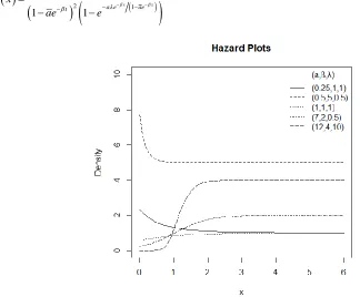
From the figure above we can see that the Extended Poisson Exponential Distribution possess increasing and decreasing failure rates depending on values of the parameters. Since for small values of shape parameters „a‟ and „λ‟ failure rate is first decreasing and then becomes constant. For large values of these shape parameters the failure rate is first increasing and then becomes constant.
3. Properties of the Distribution
In this section we have derived different properties of the EPE distribution such as Quantile function, Characteristic function and Information entropies. We have also derived Mean deviations and the density of ith order statistics.
3.1 Quantile Function
The quantile function of the distribution, obtained using (2) is given as:
1 ln
1 ln
1
q
a
x a
e q e
(5)
And the distribution median is:
1 2
1 ln
1 ln
0.5 1 a
x a
e e
3.2 Characteristic Function
Further the characteristic function of the distribution can be obtained as:
1 1
2 0
1 1
x x
itx x
e ae x
x
a e e e
t e dx
e ae
Now using the exponential series expansion we get:
2
0 0
1
1 1 ! 1
j
j x
itx x
j
x j x
e
a e e
dx
e ae j ae
Assuming
x
u e
du u dx
(6)
We get:
1
2 0 0
1 1
! 1
j it
j j
x
j
a e
t u u au dx
j e
Using the result
1 1 1 2 1 01 1 , , ; ; Re 0, Re 0, 1
x x x dxB F
(7)(Gradshteyn & Ryzhik, 2007)
The characteristic function of the EPE distribution turns out to be:
2 10
1 , 1 2,1 ; 2 ; , 1
! 1
j x
j
a e it it it
t B j F j j a for it a
j e
(8)3.3 Information Entropies
The Rényi entropy of any distribution is defined as:
1
log 1
R R
I f y dy
; 0 and 1. So for EPE distribution we have:
1 1 2 0 1 1 x x x e ae x Ra e e
f x dx e dx
e ae
Simplifying using the exponential series expansion, substitution (6) and result (7) we get:
2 1 0
, 1 2, ; 1; 0, 1.
! 1
j j j
a e
B j F j j a for a
j e
Hence the final expression for Rényi entropy is:
2 1 0
1
log , 1 2, ; 1; 0, 1.
1 1 !
j j R
j
a e
I B j F j j a for a
j e
(9)The Shannon entropy is defined as: Elogf x
For the EPE distribution we get:
1
log log log 1 2 log 1
1 x x
x
e
f x a x e ae
ae Hence
1
E log log log 1 2 log 1
1
x x
x
e
f x a E x e E ae E
ae (10)
To get E(X) we proceed:
1 1 2 0 1 1 x x x e ae xa e xe
E X e dx
Making substitution:
21 1 1 x x x x e u ae a e du dx ae (11)
1 0 1 ln 1 1 u e au e du u e
1 1 0 0ln 1 ln 1
1
u u
e
au e du u e du
e
Using 1log 1 1
i i i x x i
(12) We get
1 11 0 1 0
1 1
1
i i j
i u j u
i j
a e
u e du u e du
i j e
(13)Using Mathematica version 5.2 we get the result:
1 0
1 1 ,
Re[ ] 1. i
i u i i
u e du for j
(14) (Mathematica 5.2)Substituting (14) in equation (13) we get E(X) given as:
1 1
1
1 1 , 1 1 ,
1
i
i j
i j
e a
E X i i j j
i j e
(15) Also
2 1 1 0
1 1
1
1 1 1
x x
x x x
e ae x
x x
e a e e e
E e dx
ae
ae e ae
(16)Using the result given in (11) and simplifying we get:
11
1 1 1x x e E e ae (17) Now
1 1 2 0log 1 log 1
1 1 x x x e ae x x x
a e e
E ae ae e dx
e ae
Using (12) along with exponential series expansion, substitution (6) and result (7), equation (18) simplifies to:
2 1 1 0
1
log 1 1, 1 2, 1; 2; 1
. ! 1
i i j x
i j
a a e
E ae B i j F j i i j a for a
i j e
(19)Hence substituting (15), (17) and (19) in (10) we get the Shannon entropy as:
1 1 2 1 1 0 1E log log 1 1 , 1 1 ,
1
1
2 1 1
1, 1 2, 1; 2; 1
. ! 1
1
i
i j
i j
i i j
i j
e a
f x a i i j j
i j
e a a e
B i j F j i i j a for a
i j e
e (20)
3.4 Mean Deviations
The mean deviation about mean and median can be obtained using:
2 2 2
MD F I
2 2
MD M MF M M I M
Where we have I
y f y dy
and
0
F f y dy
.(Mahmoudi & Shiran, 2012) Considering
1 1 2 1 1 x x x e ae x ba e e
I b x e dx
e ae
Making substitution (11) we get
1 1
1 1
1 1
ln 1 ln 1
1 b b
b b
u u
e e
ae ae
e
au e du u e du
e
Using (12) along with the exponential series expansion and simplifying we get:
1 1
1 0 1 0
1 1 1 1 1 1
1 1
! 1 1 ! 1 1
1
i j m n
i i j b m n b
b b
i j m n
a
e e e
I b
i j i j ae m n m n ae
e (21)
Hence the mean deviations after using (21) are:
11 1 0
1 1 0
1 1 1
1
! 1 1
2 2 2
1 1 1 1 1
1
! 1 1
i j i i j
a e ae i j
m n m n
m n
a e
i j i j ae
e e e
MD
e e e
m n m n ae
1 1 0 1 1 01 1 1
1
! 1 1
2
1 1 1 1
1
! 1 1
i j
i i j M
M i j
m n
m n M
M m n
a e
i j i j ae
e MD M
e e
m n m n ae
(23)3.5 Order Statistics
The density of ith order statistic in a random sample of size „n‟ say Y1,…, Yn, is:
1
:
!
1
1 ! !
i n i
i n
n
f y F y F y f y
i n i
Where F(y) is the distribution function and f(y) is the density function.
Substituting the density function (1) and the distribution function (2) of EPE density we get:
1 1 1 1 1 : 2 ! 11 ! ! 1 1 1 1
x x x x
x x
i n i
a e ae a e ae x
e ae i n
x
n e e e e a e
f x e
i n i e e e ae
Using the binomial series expansion and simplifying we get:
1 2
1
2 2 1
:
0 0
1 1
!
1 ; , , 1 , 0.
1 ! ! 1 1
l n k l n i n l
n i k l
i n n k EPE
k l
e e
n i n k
n
f x f x a l x
k l
i n i l e
(24) Where
11 1 1
2 1
1
; , , 1
1 1
x x
l x
l e ae
EPE l
x
a l e
f x a l e
e ae
Since (24) is a linear combination of the Extended Poisson Exponential (EPE) densities so we can obtain the mean of the density function of ith order statistic in terms of the mean of EPE distribution as follows:
2 2 1 1
1 1
:
0 0
1
1 1 , 1
1 1
1 !
1 ! ! 1 1 1
1 1 , 1
1
i i n k i l n k i
n i n l i
i n n k
k l
j j j
a
i i l
i l
e
n i n k
n E X
k l
i n i l e
j j l
j l
(25)4. Estimation of Parameters
Here we dealt with the parameter estimation problem for the Extended Poisson-Exponential distribution.
The log-likelihood function for a sample of size „n‟ given as yy1,...,ynfrom the
distribution can be written as:
1 1 1
1
ln ln 1 2 ln 1
1 i i
i x
n n n
x
i x
i i i
e
l n a n x n e ae
ae
Now differentiating the log-likelihood function w.r.t. the parameters we get the given normal equations:
21 1 1 2 1 1 i i i i i x x x n n x x i i e e
l n e
a a ae ae
(27)
21 1 1
2 1 1 i i i i x x
n n n
i i
i x x
i i i
l n x e x e
x a a
ae ae
(28)
1 1 1 1 i i x n x i el n ne
n e ae
(29)Equating these expressions to zero and solving the equations we can get the Maximum Likelihood Estimates (MLEs) of the distribution. Here we do not have any closed form expressions for MLEs so numerical maximization through iterative procedures have to be used to get the MLEs.
In order to draw large sample inferences for the distribution we make use of the fact that
( )( ̂ )D ( )
as n approaches to infinity, when the suitable regularity conditions are satisfied. Here I is the identity matrix and ( ) is the Choleski decomposition of the Fisher‟s Information matrix ( ), i.e. ( ) ( ) ( ).
(Cox & Hinkley, 1974)
The asymptotic variance-covariance matrix of the MLEs is the inverse of the Fisher‟s Information matrix which can be estimated by the inverse of the observed information matrix. And these estimates can be used to construct the asymptotic confidence intervals and to draw inferences about the parameters asymptotically.
The Fisher‟s Information matrix is:
2 2 2
2
2 2 2
2
2 2 2
2
n
l l l
E E E
a a
a
l l l
I E E E
a
l l l
E E E
a
And all the second order derivatives involved in the above matrix are:
2
2 2
2 2 2 3
1 1 1 2 2 1 1 i i i i i x x x n n x x i i e e
l n e
a a ae ae
,
2 2 1 1 1 i i i x x n x i e e l a ae
2 2 3 1 1 1 2 2 1 1i i i
i
i i
x x x
x n n i i x x i i
x e e ae
l x e
a ae ae
,
2 2 1 1 i i x n i x il x e
a ae
,
2 2 22 2 3
1 1
1 2 1
2
1 1
i i i i
i
i
x x x x
n n
i i
x
x
i i
x e ae x e ae
l n a ae ae
,
2 22 2 2
1
l n ne
5. Real Data Application
Extended Poisson-Exponential distribution has been fitted to real data sets in order to determine whether it provides a good fit or not. Comparison of the new model with Poisson Exponential distribution has been made for three different data sets.
Data set 1:
The data employed consists of 63 observations on “the strength of 1.5 cm glass fibers, measured at the National Physical Laboratory, England”. The data set is given as:
0.55, 0.93, 1.25, 1.36, 1.49, 1.52, 1.58, 1.61, 1.64, 1.68, 1.73, 1.81, 2 ,0.74, 1.04, 1.27, 1.39, 1.49, 1.53, 1.59, 1.61, 1.66, 1.68, 1.76, 1.82, 2.01, 0.77, 1.11, 1.28, 1.42, 1.5, 1.54, 1.6, 1.62, 1.66, 1.69, 1.76, 1.84, 2.24, 0.81, 1.13, 1.29, 1.48, 1.5, 1.55, 1.61, 1.62, 1.66, 1.7, 1.77, 1.84, 0.84, 1.24, 1.3, 1.48, 1.51, 1.55, 1.61, 1.63, 1.67, 1.7, 1.78, 1.89.
(Barreto-Souza, Santos, & Cordeiro, 2008)
We have fitted the Extended Poisson Exponential (EPE) distribution, and the Poisson-Exponential (PE) distribution, introduced by Cancho et al. (2011), to this data set. The Maximum Likelihood Estimates and their log likelihood values are given as:
For EPE distribution:
̂ , ̂ , ̂ , ̂ .
For PE distribution:
̂ ̂ , ̂ .
Now we will test EPE distribution against PE distribution for better fit for the given data set. The null and alternative hypotheses to be tested are: ( ) against
( ). For the given hypothesis the value of Likelihood ratio test statistic is
25.98732 with corresponding P-value 0.0001. Hence at this P-value we reject the null hypothesis at the usual level of significance and conclude that the EPE distribution provides a better fit than the PE distribution for the given data set.
Data Set 2:
This data set contain 101 observations on fatigue life of 6061-T6 aluminum coupons cut parallel to the direction of rolling and oscillated at 18 cycles per second. The observations are:
70, 90, 96, 97, 99, 100, 103, 104, 104, 105, 107, 108, 108, 108, 109, 109, 112, 112, 113, 114, 114, 114, 116, 119, 120, 120, 120, 121, 121, 123, 124, 124, 124, 124, 124, 128, 128, 129, 129, 130, 130, 130, 131, 131, 131, 131, 131, 132, 132, 132, 133, 134, 134, 134, 134, 136, 136, 137, 138, 138, 138, 139, 139, 141, 141, 142, 142, 142, 142, 142, 142, 144, 144, 145, 146, 148, 148, 149, 151, 151, 152, 155, 156, 157, 157, 157, 157, 158, 159, 162, 163, 163, 164, 166, 166, 168, 170, 174, 201, 212.
Again we have fitted the two distributions, the EPE distribution and the PE distribution to this data set and obtained the following results:
For EPE distribution:
̂ , ̂ , ̂ , ̂
.
For PE distribution:
̂ ̂ , ̂ .
The Likelihood Ratio test has been used to test the hypotheses ( ) vs.
( ) with the value of test statistic equals to 10.4742 with P-value 0.0012.
Hence at 0.05 level of significance we can conclude that the EPE distribution performs significantly better than the PE distribution for this data set.
Data Set 3:
This data set reports the remission times (in months) of 128 bladder cancer patients. The data are:
0.08, 2.09, 3.48, 4.87, 6.94 , 8.66, 13.11, 23.63, 0.20, 2.23, 3.52, 4.98, 6.97, 9.02, 13.29 , 0.40, 2.26, 3.57, 5.06, 7.09, 9.22, 13.80, 25.74, 0.50, 2.46 , 3.64, 5.09, 7.26, 9.47, 14.24, 25.82, 0.51, 2.54, 3.70, 5.17 , 7.28, 9.74, 14.76, 26.31, 0.81, 2.62, 3.82, 5.32, 7.32, 10.06 , 14.77, 32.15, 2.64, 3.88, 5.32, 7.39, 10.34, 14.83, 34.26, 0.90 , 2.69, 4.18, 5.34, 7.59, 10.66, 15.96, 36.66, 1.05, 2.69, 4.23 , 5.41, 7.62, 10.75, 16.62, 43.01, 1.19, 2.75, 4.26, 5.41, 7.63 , 17.12, 46.12, 1.26, 2.83, 4.33, 5.49, 7.66, 11.25, 17.14, 79.05 , 1.35, 2.87, 5.62, 7.87, 11.64, 17.36, 1.40, 3.02, 4.34, 5.71 , 7.93, 11.79, 18.10, 1.46, 4.40, 5.85, 8.26, 11.98, 19.13, 1.76 , 3.25, 4.50, 6.25, 8.37, 12.02, 2.02, 3.31, 4.51, 6.54, 8.53 , 12.03, 20.28, 2.02, 3.36, 6.76, 12.07, 21.73, 2.07, 3.36, 6.93 , 8.65, 12.63, 22.69.
(Lee & Wang, 2003)
The EPE distribution and PE distribution were fitted to this data set also. The parameter estimates and Log-Likelihood values for two distributions are:
For EPE distribution:
̂ , ̂ , ̂ , ̂ .
For PE distribution:
̂ ̂ , ̂ .
Figure 3: The Glass Fiber strength data and the fitted densities.
Figure 4: The Aluminum coupons fatigue life data and the fitted densities.
Figure 5: The Bladder cancer remission time data and the fitted densities.
6. Concluding Remarks
References
1. Adamidis, K., Dimitrakopoulou, T., & Loukas, S. (2005). On An Extension Of The Exponential-Geometric Distribution. Statistics & Probability Letters, 73, 259–269. Doi:10.1016/J.Spl.2005.03.013
2. Adamidis, K., & Loukas, S. (1998). A Lifetime Distribution With Decreasing Failure Rate. Statistics & Probability Letters, 39, 35-42.
3. Asgharzadeh, A., Bakouch, H. S., Nadarajah, S., & Esmaeili, L. (2014). A New Family Of Compound Lifetime Distributions. Kybernetika, 50(1), 142-169. Retrieved From Http://Dml.Cz/Dmlcz/143768
4. Bakouch, H. S., Ristić, M. M., Asgharzadeh, A., Esmaily, L., & Al-Zahrani, B. M. (2012). An Exponentiated Exponential Binomial Distribution With Application. Statistics & Probability Letters, 82(6), 1067–1081. Doi:10.1016/J.Spl.2012.03.004
5. Barreto-Souza, W., & Bakouch, H. S. (2010). A New Lifetime Model With Decreasing Failure Rate. Retrieved From http://Arxiv:1007.0238v1
6. Barreto-Souza, W., Santos, A. H., & Cordeiro, G. M. (2008). The Beta Generalized Exponential Distribution. Retrieved From http://Arxiv.Org/Abs/0809.1889v1
7. Birnbaum, Z.W., Saunders, S.C., 1969. Estimation for a Family of Life Distributions with Applications to Fatigue. Journal of Applied Probability, 6, 328-347.
8. Cancho, V. G., Louzada-Neto, F., & Barriga, G. D. (2011). The Poisson-Exponential Lifetime Distribution. Computational Statistics And Data Analysis, 55, 677-686.
9. Cordeiro, G. M., & Silva, R. B. (2014). The Complementary Extended Weibull Power Series Class Of Distributions. Ciência E Natura, 36, 1–13. Doi:10.5902/2179460X13194
10. Cox, D. R., & Hinkley, D. (1974). Theoretical Statistics. Chapman And Hall. 11. Gradshteyn, S.I. And Ryzhik, M.I. (2007). Table Of Integrals, Series And
Products.Seventh Edition.
12. Hemmati, F., Khorram, E., & Rezakhah, S. (2011). A New Three-Parameter Ageing Distribution. Journal Of Statistical Planning And Inference, 141, 2266– 2275.
13. Kus, C. (2007). A New Lifetime Distribution. Computational Statistics & Data
Analysis, 51, 4497 – 4509.
14. Lee, E.T., Wang, J.W. (2003). Statistical Methods for Survival Data Analysis, 3rd edition. Wiley: New York.
16. Mahmoudi, E., & Shiran, M. (2012). Exponentiated Weibull-Geometric Distribution And Its Applications. Elsevier. Retrieved From Http://Arxiv.Org/Abs/1206.4008v1
17. Mahmoudi, E., & Zakerzadeh, H. (2010). Generalized Poisson–Lindley Distribution. Communications In Statistics - Theory And Methods, 39(10), 1785-1798. Doi:10.1080/03610920902898514
18. Marshall, A.W., & Olkin, I. (1997). A New Method For Adding A Parameter To A Family Of Distributions With Application To The Exponential And Weibull
Families. Biometrika, 84(3), 641-652.
http://Dx.Doi.Org/10.1093/Biomet/84.3.641
19. Preda, V., Panaitescu, E., & Ciumara, R. (2011). The Modified Exponential-Poisson Distribution. Proceedings Of The Romanian Academy, Series A, 12(1),
22–29.
20. Tahmasbi, R., & Rezaei, S. (2008). A Two-Parameter Lifetime Distribution With Decreasing Failure Rate. Computational Statistics And Data Analysis, 52, 3889– 3901.