Contrast effects on sequence assessments
Zhifang Ni
A thesis submitted to the Department of Management of
the London School of Economics and Political Science for
the degree of Doctor of Philosophy
Declaration
I certify that the thesis I have presented for examination for the PhD degree of the London School of Economics and Political Science is solely my own work other than where I have clearly indicated that it is the work of others (in which case the extent of any work carried out jointly by me and any other person is clearly identified in it). This thesis benefits from discussions with colleagues, my supervisor and the two examiners. However, where their contributions are noted, all views remain my own. The copyright of this thesis rests with the author. Quotation from it is permitted, provided that full acknowledgement is made. This thesis may not be reproduced without the prior written consent of the author.
Contrast effects on sequence assessments
Abstract
Loewenstein and his colleagues found divergent preferences for outcomes assessed in isolation versus those embedded in a sequence, i.e. discounting isolated future outcomes versus preferences for increasing and constant sequences. They also found long intervals (i.e. the difference between time delays) rather than long time delays (i.e. the temporal distance from the present) had a detrimental effect on preference for improvement. This thesis proposes a descriptive model of sequence preferences, namely the contrasts model, which acknowledges the difference between interval and delay. The idea is that delay and interval are two different kinds of variables. Delay is non-relational and describes characteristics of individual outcomes, whereas interval is relational and describes characteristics of outcomes in relation to one another. Built on this idea, the contrasts model assumes that the value of a sequence consists of a non-relational part (the endowment value), which is a function of delay and nominal value of the component outcomes and a relational part (the contrast value), which is a function of the signed value difference between the outcomes, their interval and domain relatedness (i.e. whether or not the outcomes share the same domain). Delay and interval influence the endowment and the contrast respectively. Empirical investigations provide evidence for the contrasts model. Decision makers are capable of distinguishing between influences of delay and interval even when the two coincide and exert conflicting influences. Experiments using both money and non-monetary outcomes also show that preferences for improvement can be made more pronounced by shortening intervals and/or enhancing relatedness between the outcomes.
Acknowledgements
I would like to thank Prof Daniel Read for his supervision and my two examiners, Professor Peter Ayton and Professor Nick Chater, for their invaluable comments that improve the quality of this work.
My parents and all my friends have also been extremely supportive and helpful throughout the long period during which I conduct this research. I especially wish to thank Professor Zhengmin Tong for his assistance in conducting two experiments in China.
Table of Contents
Page
Title 1
Declaration 2
Abstract 3
Acknowledgements 4
Table of Contents 5
List of Tables 9
List of Illustrations 10
Table of notations 11
Chapter 1 INTRODUCTION 12
Chapter 2 SEQUENCE PREFERENCES 19
2.0 Introduction 19
2.1 The discounted utility model (DU) 19
2.1.1 Preferences for isolated outcomes 21
2.2 Sequence preferences 23
2.2.1 Improvement 23
2.2.2 Spreading 27
2.3 Perceptions of sequences 30
2.3.1 Continuous sequences 32
2.3.2 Continuous versus discrete sequences 34
2.4 Influences of choice bracketing 36
2.5 Summary 37
Chapter 3 DELAY AND INTERVAL 38
3.0 Introduction 38
3.1 Delay as psychological distance 38
3.2 Similarity 40
3.2.1 Grouping 41
3.2.2 Context-dependency 41
3.2.3 Decision weights 45
3.3 Implications for time preferences 47
3.3.1 Integrity 47
3.3.2 Time contraction 49
3.3.3 The “similarity effect” 50
3.3.4 Assessment mode 51
Page
3.5 Summary 54
Chapter 4 CONTEXT EFFECTS 55
4.0 Introduction 55
4.1 Context effects 56
4.1.1 Accessibility-applicability 57
4.1.2 The Inclusion/Exclusion Model (IEM) 58
4.1.3 Interval 60
4.2 Implications for time preferences 62
4.2.1 The endowment-contrast effects model 63
4.2.2 The consumption-contrast effects model 65
4.2.3 Discussion 66
4.3 Summary 68
Chapter 5 CHOICE BRACKETING 69
5.0 Introduction 69
5.1 Bracketing 69
5.1.1 Narrow bracketing prevails 71
5.1.2 Overbracketing 74
5.1.3 Decision versus experienced utility 76
5.2 Bracketing and sequence judgments 77
5.2.1 Discussion 79
5.3 Summary 81
Chapter 6 THE CONTRASTS MODEL 82
6.0 Introduction 82
6.1 Tversky and Griffin (1991) 82
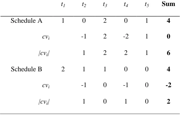
6.2 Loewenstein and Prelec (1993) 83
6.2.1 An example 85
6.3 The contrasts model 84
6.4 Model comparisons 89
6.4.1 A validation of the contrasts model 93
6.4.2 Incorporating time discounting 96
6.4 Looking ahead 99
Chapter 7 THE RANKING TASK 102
7.0 Introduction 102
7.1 The ranking task 102
Methods 102
Page
Discussion 108
7.2 Summary 109
Chapter 8 INTRA- AND INTER-PERSONAL CONTRASTS 111
8.0 Introduction 111
8.1 General methods 111
8.2 The sequence judgment task 113
Methods 114
Results 115
Discussion 119
8.3 The interpersonal (social) judgment task 122
Methods 123
Results 124
Discussion 128
8.4 General discussion 129
8.5 Summary 131
Chapter 9 THE SCHEDULING TASK 132
9.0 Introduction 132
9.1 The scheduling task 132
9.1.1 Scheduling task I 133
Methods 133
Results 135
Discussion 137
9.1.2 Scheduling task II 139
Methods 139
Results 140
Discussion 147
9.2 General discussion 148
9.3 Summary 150
Chapter 10 THE HAPPINESS TASK 151
10.0 Introduction 151
10.1 The happiness task 151
Methods 153
Results & discussion 154
Task 2 results 155
Task 1 results 157
Page
Individual-level analysis of sequence ratings 166
Model comparison 169
10.2 Summary 170
Chapter 11 FINAL REMARKS 171
11.1 Introduction 171
11.2 Positive, null and negative time preferences 173
11.3 Interval and relatedness 174
11.4 Delay 176
11.5 Dual influences 176
11.6 Other findings 177
REFERENCES 179
APPENDIXES
Appendix A – Results of the model comparison (Chapter 6) 193
Appendix B – Questionnaire of the ranking task 194
Appendix C – Questionnaire of the sequence judgment task 195 Appendix D – Questionnaire of the interpersonal judgment task 197
Appendix E – Questionnaire of the scheduling task I 198
Appendix F – Questionnaire of the scheduling task II 202
List of Tables
Page
Table 3.1 A choice between two non-dominant options. 46
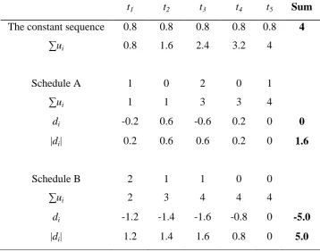
Table 6.1 Computations of LP for Schedule A and B (Eq. 6.2). 86
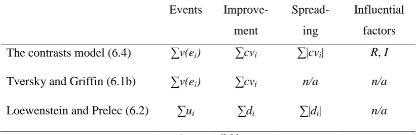
Table 6.2 A comparison of the contrasts model, TG and LP. 89
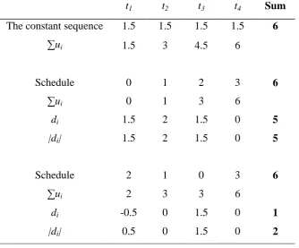
Table 6.3a Computation details of (0,1,2,3) and (2,1,3,0): LP. 91 Table 6.3b Computation details of (0,1,2,3) and (2,1,3,0): the contrasts model. 91
Table 6.4 Computations of the contrasts model (Eq.6.4) 94
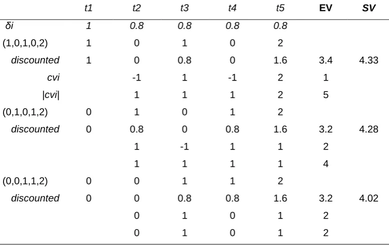
Table 6.5 Performance of LP and the contrasts model (Eq.6.4) 95 Table 6.6 Computations of the discounting-adjusted contrasts model (Eq.6.5) 97 Table 6.7 Influences of delay on preference for improvement 98
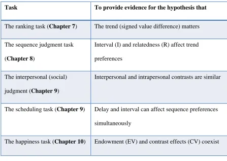
Table 6.8 Overview of the experiments. 101
Table 7.1 Sequences used in the ranking task 103
Table 7.2a Rankings of the “mixed” group (n=53) 105
Table 7.2b Rankings of the “positive” group (n=56) 105
Table 8.1 Assessment of the increasing sequences 115
Table 8.2a Mean Ratings and standard deviations (N=138) 116
Table 8.2b ANOVA model results (within-subjects) 116
Table 8.3 The ownership effect in the sequence judgment task 119 Table 8.4 A sample matrix of the interpersonal judgment task 123
Table 8.5a Mean Ratings and standard deviations (n=27) 124
Table 8.5b ANOVA model results 125
Table 9.1 Choice percentages and mean ratings in Scheduling Task I 136
Table 9.2 Choice percentages in Scheduling Task II. 141
Table 9.3 Mean ratings in Scheduling Task II. 143
Table 9.1 Impact of delay on sequence preferences in Scheduling Task II 144
Table 9.5a Males‟ time preferences in Scheduling Task II 145
Table 9.5b Females‟ time preferences in Scheduling Task II 145
Table 10.1 The design of the happiness task 152
Table 10.2 Results of Task 2 (n=18) 155
Table 10.3 Predictions of sequence preferences for the happiness task 156 Table 10.4 The results of Task 1 and the predictions of the contrasts model. 158 Table 10.5a The impact of relatedness and interval for the positive pairs 159 Table 10.5b The impact of relatedness and interval for the negative pairs 159
Table 10.5c The impact of discounting 162
Table 10.6 Results of the happiness task III (n=21) 163
Table 10.7 Ratings of the four pairs of events observed in Task 1. 164 Table 10.8 Results of the logistic regression for Task 3 results 166
Table 10.9 Results of the Solver analysis 167
Table 10.10 A comparison of model predictions 169
Page
List of Illustrations
Page
Figure 3.1 Judgments of similarity when the “range” varies 42 Figure 3.2 Judgments of similarity when the “frequency” varies 43 Figure 4.1 The mean satisfaction ratings in Tversky & Griffin (1991). 65 Figure 7.1 Distribution of the observed rank-orders in the ranking task 106
Figure 8.1 Domain × Interval × Trend 117
Figure 8.2 The effect of situation ownership 119
Figure 8.3 The two-way interactions 126
Figure 8.4 The three-way interaction: Interval × Amount × Trend 127 Figure 9.1a % choosing (Friends, Aunt) in Scheduling Task I 136 Figure 9.1b Means and sds of the ratings in Scheduling Task I 136 Figure 9.2 A time-line graph representation of the increasing (Aunt, Friends) 140 Figure 9.3 % Participants show different time preferences in Scheduling Task II 141
Figure 9.4 Means and sds observed in Scheduling Task II 143
Figure 9.5 The gender effect in Scheduling Task II 145
Figure 10.1 Mean ratings of the sequences (n=41) 158
Table of Notations
Notation Description
r discount rate
discount factor or discount parameter in the contrasts model
β parameter of the improvement predictor in LP and the contrasts model
σ parameter of the spreading predictor in LP
σ' parameter of the spreading predictor in the contrast model
{} brackets of choice, e.g. { puddings for Monday, puddings for Saturday} (e1,e2, …en) a temporal sequence that consists of n events/outcomes
CLT the Construal Level Theory CV the contrast value of a sequence DU the Discounted Utility model EV the endowment value of a sequence IEM the Inclusion/Exclusion model
LP Loewenstein and Prelec‟s (1993) model of sequence preferences NV the nominal value of a sequence
Chapter 1 INTRODUCTION
A sequence is a series of outcomes spaced over time (Loewenstein & Prelec, 1993). Sequences are ubiquitous. Almost all decisions have costs and benefits extended into the future. These include important life-time decisions, e.g. schooling and marriage, as well as seemingly trivial ones, e.g. whether to snack on an apple or a chocolate bar. Chocolate bars may bring higher immediate pleasure; apples however offer greater long-term benefits to health.
Such predictions contradict a large body of empirical evidence. While it is true that people prefer gains earlier rather than later, they also prefer increasing sequences to decreasing ones. The so-called preference for improvement has been observed in a variety of domains for both positive and negative outcomes, monetary and non-monetary outcomes (Chapman, 1996; Guyse, Keller, & Eppel, 2002; Hsee & Abelson, 1991; Loewenstein & Prelec, 1991, 1993; Loewenstein & Sicherman, 1991; Read & Powell, 2002; Ross & Simonson, 1991; Stevenson, 1993); it even applies to retrospective assessments of aversive experiences, such as pains and discomfort (Kahneman, Fredrickson, Schreiber, & Redelmeier, 1993; Varey & Kahneman, 1992). In addition to this, people sometime prefer to spread outcomes evenly across time. Loewenstein and Prelec (1993) called these two kinds of preferences, i.e. preference for improvement and preference for spreading, the two modal sequence preferences. Modal sequence preferences imply time preferences that are non-positive.
The divergent time preferences result in part from how one makes decisions, or the level of choice bracketing (Read, Loewenstein & Rabin, 1999). Under narrow bracketing, the decisions are made in isolation, whereas under broad bracketing, the decisions are made at the same time, taking into account effects of one decision exerts on other decisions. Outcomes presented in isolation versus in a sequence foster narrow and broad bracketing respectively. That people tend to bracket choices narrowly exacerbates positive time preference for isolated outcomes.
The co-existence of positive and negative time preferences does not represent the only challenge faced by DU. A more fundamental problem is that features important for sequence assessments do not exist for isolated outcomes. These include the so-called “Gestalt characteristics” or sequence-level characteristics such as the
Hsee, Salovey, & Abelson, 1994), the peak and end values (Fredrickson & Kahneman, 1993; Kahneman, et al., 1993; Ross & Simonson, 1991). Also important are factors that operate on people‟s perceptions about sequences, which include the length of
interval (Loewenstein & Prelec, 1991, 1993), i.e. the difference between the two delays, as well as the ways in which sequences are partitioned (Ariely & Zauberman, 2000, 2003). Notably, influences of interval and delay diverge systematically. Interval rather than delay determines outcome integrity, or the degree to which outcomes are perceived as a whole (Loewenstein & Prelec, 1993), which in turn affects preference for improvement.
As an alternative to DU, Loewenstein and Prelec (1993) proposed a model (henceforth LP) that described sequence preferences based on the idea that people derive utility not only from direct experiences, but also from memory and anticipation
(Loewenstein, 1987; Loewenstein & Elster, 1992). A desirable event, once experienced, no longer provides a source for anticipatory utility. Worse, it may serve as a comparison standard and in so doing, decrease the perceived attractiveness of later, related experiences. The opposite holds for negative experiences. This kind of “triple-counting” of utility, i.e. before, during and after the actual experience, explains why people may choose to delay a positive experience while at the same time expedite a negative one.
relationship between the outcomes. Delay measures psychological distance of an isolated outcome and determines outcome representation and assessments. I discuss impact of delay using Trope and Liberman‟s (2000, 2003) Construal Level Theory. By contrast, interval reflects how similar outcomes are perceived in terms of time. Similarity determines grouping and categorization (Higgins & Brendl, 1995; Kahneman & Tversky, 1982; Tversky, 1977). This provides an account for the interval effect on outcome integrity (Kahneman & Tversky, 1979), with implications for how people perceive a set of outcomes, how these outcomes interact with each other (Schwarz & Bless, 1992) as well as the strength of such interactions (Higgins & Brendl, 1995). None of these are applicable to delay.
To incorporate these ideas into describing sequence preferences, I elaborate on Tversky and Griffin‟s (1991) endowment and contrast effects framework (or TG). It assumes that the way temporal outcomes interact with each other conforms to the so-called context effects, i.e. influences of the decision context on judgments. The idea is that each sequence outcome, except for the very last, exerts dual influences on the assessment of the entire sequence – a direct endowment effect that reflects its true worth and an indirect contrast effect that affects the assessment of later, related outcomes. The difference between endowments and contrasts parallel the one between delay and interval. Endowments are specific to individual outcomes whereas contrasts arise between outcomes. In other words, endowments and contrasts are non-relational
and relational effects respectively. It is therefore logical to assume that delay affects the endowment but not the contrast and interval affects the contrast but not the endowment. The “contrasts model” of sequence preferences thus distinguishes between the influences of the two temporal variables. The same logic predicts that
are perceived as of the same kind, exerts similar influences as interval rather than delay.
Exactly how interval and relatedness affect contrast effects can be understood from research on context effects. Based on this research, contrast effects are more pronounced between more related outcomes and/or outcomes with shorter time intervals. Delay, on the other hand, fosters discounting; the longer the delay, the greater the discounting, the smaller the endowment value will be. A sequence is more attractive if it has a large endowment and/or a large contrast. Intervals exert dual influences on sequence preferences because for a series of future outcomes, shorter intervals imply shorter time delays. Thus shorter intervals not only enhance contrast effect but also entail less discounting.
The rest of the thesis illustrates these ideas. The first four chapters, from Chapter 2 to 5, lay the theoretical foundation of the contrasts model. Chapter 2 reviews empirical findings of time preferences, i.e. preferences for isolated outcomes and preferences for sequences, highlights the difference between the two, and examines psychological mechanisms underlying sequence preferences. Chapter 3 explores the difference between interval and delay, derived from the Construal Level Theory and research on similarity. Chapter 4 discusses context effects and show influences of interval and delay. Chapter 5 discusses influences of choice bracketing on perceptions and assessments of sequences.
effects depend on the signed value difference between the (adjacent) outcomes, their lengths of interval and degree of relatedness.
Chapter 7 to 10 report experiments that test these predictions. The ranking task
in Chapter 7 tests trend effect, i.e. the magnitude of improvement (deterioration) as captured in the signed value difference. The sequence judgment task in Chapter 8 examines the influences of relatedness and interval on contrast effects. That is, as the outcomes become related or temporally nearer, whether the value discrepancy between increasing and decreasing sequences (endowment) would become larger. One implication of the contrast effects is that interpersonal contrasts (i.e. contrasts between outcomes received by different individuals) parallel intrapersonal ones (i.e. contrasts between outcomes embedded in a sequence). The interpersonal judgment task, also reported in Chapter 8, adopts the same design as the sequence (intrapersonal) judgment task. The difference is that the “context” is now a gain received by another individual rather than by the same individual at a different time. Comparing and contrasting the results of these two studies provide insights into contrast effects in the two different types of judgment tasks. A parallel between the two, if found, would provide support for the approach of describing sequence preferences by borrowing insights from research into context effects.
depends on delays) interferes with preference for improvement (which depends on intervals).
Chapter 2
SEQUENCE PREFERENCES
2.0 Introduction
Over the years the question of how value changes over time has stimulated fruitful research in a wide range of disciplines, including psychology (Read & Loewenstein, 2000), behavioural economics (Thaler, 1981), political sciences (Schelling, 1984), and neuroeconomics (Camerer, Loewenstein, & Prelec, 2005). This investigation employed a diverse range of methods and techniques, including real choices, laboratory experiments, econometrics and even medical test such as functional Magnetic Resonance Imaging. Loewenstein, Read and Baumeister‟s book (2003) surveys recent developments in the field. This body of research lends insight into people‟s divergent time preferences for isolated outcomes versus for sequences, as well as the difference between interval and delay. This chapter examines this topic. My plan is this. I start by discussing the Discounted Utility model (DU, Koopmans, 1960; Samuelson, 1937), which remains the framework of choice for predicting preferences for future outcomes. I show how preferences for isolated outcomes differ systematically from preferences for sequences. Differences between interval and delay emerge. I then examine psychological mechanisms underlying the two modal sequence preferences, i.e. preferences for improvement and spreading. In the end of the chapter, I introduce the notion of choice bracketing to show how the way people make choices affects decisions.
2.1 The discounted utility model (DU)
stream of future consequences is a function of utility pertaining to individual outcomes. That is, V=f(u0, u1, …ut), where ut denotes the consumption utility at time t. As a particular instantiation of this general model, DU assumes outcome independence, meaning that the value of an outcome is independent of other outcomes in the same sequence. This assumption, in combination with a series of technical axioms collectively known as “completeness”, implies the General Additively Separable representation (Loewenstein, 1992):
V= ∑d(t)ut, --- (2.1)
In Eq.2.1, d(t) is a discount function that reflects the impact of time delay t on the value of an outcome received at time t. Two common representations of discount function are discount factor, denoted as δt, and discount rate, denoted as rt. Discount factor captures the proportion of value remained after an outcome has been delayed by a standard time unit (t), e.g. a year; discount rate is the percentage by which the value is reduced for each time period. The relationship between the two discount parameters is straightforward, i.e. δt=1-rt. For instance, a yearly discount factor of 0.9
implies that £100 to be received a year from now is worth £90 now; and a yearly discount rate of 10% implies that in a year‟s time £100 now will be worth 90% (=1-10%) of its original worth, or £90. An individual is said to have positive (negative)
time preference if her discount rates are positive (negative), or if her discount factors are less (greater) than 1. For such individuals, we say that value decays (accrues) over time.
an individual‟s idiosyncratic time preferences. The idea is that the existence of capital markets allows individuals to make intertemporal trade-offs – one can speed up a future consumption or delay an immediate one to the extent that his or her marginal rate of time preference would always equal the interest rate for money (Loewenstein & Thaler, 1989). This implies a fixed relationship between discount factor and market interest rates, i.e. δt=1/(1+x), where x is the prevailing market interest rate. Inserting
this into Eq.2.1 produces
n
t
t x u
V t
0 (1 )
, which is the well-known expression for
computing the net present value (NPV) of a sequence of future incomes.
2.1.1 Preferences for isolated outcomes
Theoretically, the NPV expression is applicable to monetary outcomes or non-monetary outcomes measurable by money. It makes two predictions: people discount
future outcomes and have consistent time preferences. Discounting is based on the fact that market interest rates are almost universally positive. Since any unspent money can be saved or invested to earn interests, future money should be valued less than immediate money. Time consistency means one‟s later preferences “confirm” rather than contradict his earlier preferences (Frederick, et al., 2002). This stems from the use of a constant discount parameter regardless of time delay. In the NPV formulation, this discount rate is the prevailing market interest rate for all time periods, no matter how distant or near the outcomes are.
Loewenstein and Prelec (1993) showed that 82% of their participants who enjoyed French food preferred to have a French dinner in one month rather than in two months.
On the other hand, “inconsistent” behaviours are abundant in real life – we
plan to work on a paper/go on a diet/start exercising only change our mind in the presence of more tempting alternatives, e.g. surfing internet/having desserts/dozing off. Hyperbolic discounting (Ainslie, 1992) refers to the empirical finding that discounting is slower (i.e. a larger discount factor or a smaller discount rate) when the delay is longer. For instance, Thaler (1981) asked people to state the future value of amounts of money available now, if they were delayed by times varying from 3 months to 10 years. Given a present amount of $15, people‟s implicit discount rate decreased from 277% when the delay was three months to 19% when the delay was ten years. Dozens of follow-up studies found similar results (Read, 2004). Hyperbolic discounting predicts time inconsistency, i.e. preference reversals between a smaller sooner option (SS), e.g. having desserts, and a larger later option (LL), e.g. exercising, when both options are delayed. The idea is that the shorter the delay, the faster the discounting. Thus, compared to LL, SS loses value at a faster rate when both options are delayed. People who prefer SS to LL when both options are near may prefer LL to
SS instead when both are distant (Ainslie, 1992; but see Read, 2001b).
2.2 Sequence preferences
In sharp contrast to the “impatience” people exhibit towards isolated outcomes is their patience when facing a set of temporally distributed outcomes – people sometimes want to save the best till last, rather than to have them as soon as possible, or they want to spread outcomes evenly across time. Loewenstein and Prelec (1993) refer to preference for improvement and preference for spreading as the two modal
sequence preferences. In what follows, I review each in turn and examine their underlying mechanisms.
2.2.1 Improvement
Example 2.1 (n=82)
Choice 1 Choice
A. French dinner in this month [80%] B. French dinner in next month [20%]
Choice 2 This month Next month Choice C. French dinner Greek dinner [43%] D. Greek dinner French dinner [57%]
Ross and Simonson (1991) reported similar findings. Their participants strongly preferred sequences of gambles that ended with a gain (lose $15, then win $85) to those that ended with a loss (e.g. win $85, then lose $15), despite the same expected payoffs of the gambles. They subsequently referred to this finding as a preference for “happy endings”. Hsee and Abelson (1991) further showed that their undergraduate participants preferred a fast rise in salary and academic performance to a slow rise, as well as a slow fall to a fast fall. That is, preference for improvement is moderated by the velocity in which the value changes over time (Hsee & Abelson, 1991). Later investigation by Hsee, Salovey and Abelson (1994) found that the impact of velocity was particularly salient towards the end of a sequence. That is, satisfaction was higher if the rate of change increased for increasing sequences and decreased for decreasing sequences.
dinners (Loewenstein & Prelec, 1991), gambling (Ross & Simonson, 1991), academic performances (Hsee & Abelson, 1991), health states (Chapman, 1996; Read & Powell, 2002), environmental goods (Guyse, et al., 2002). It holds even when people search for an ordered set (Diehl & Zauberman, 2005) and make retrospective assessments of aversive experiences, such as pains and discomfort (Kahneman, et al., 1993; Varey & Kahneman, 1992).
Why is preference for improvement so prevalent? It seems that this preference is overdetermined, motivated by multiple psychological mechanisms including
savouring and dread (Loewenstein, 1987; Loewenstein & Elster, 1992), adaptation (Helson, 1964), loss aversion (Kahneman & Tversky, 1979), and the closely related
contrast effects (Loewenstein & Elster, 1992; Mussweiler & Strack, 2000; Schwarz & Bless, 1992a; Tversky & Griffin, 1991).
First, Loewenstein (1987) argued that people derive utility from anticipatory savouring and dread. His participants preferred to delay a kiss from their favourite movie star for a few days while to receive unpleasant electric shocks as soon as possible. Loewenstein (1987) explained that these actions enhanced one‟s satisfaction by permitting the accumulation of utility and avoiding that of disutility. This implies that people will perceive the improving sequence of events (immediate shock, delayed kiss)1 to be more attractive than the deteriorating sequence of events (immediate kiss, delayed shock).
Second, adaptation-level theory posits that people tend to adapt to on-going stimuli over time and to evaluate new stimuli relative to their adaptation-level. Kahneman and Tversky‟s (1979) notion of loss-aversion refers to the observation that a loss is more painful than a gain of the same magnitude. For sequences, if people
1
adapt to the most recent level of stimuli they experience, then sequences that strictly improve afford a continuous series of upward shift, perceived as gains. By contrast, decreasing sequences provide a series of losses. Since losses loom larger than gains, increasing sequences are particularly attractive compared to decreasing sequences.
Third, Tversky and Griffin (1991) argue that a hedonic event may contrast with a later event and change its perceived attractiveness. The direction of these contrasts is predominantly backward (Bruine de Bruin & Keren, 2003; Loewenstein & Elster, 1992; Prelec & Loewenstein, 1991); that is, an earlier event serves as a comparison standard for a later event, rather than forward, or the other way around. Backward contrast effects predict that having inferior experiences earlier enhances the attractiveness of later, superior experiences (Heyman, Mellers, Tishcenko, & Schwartz, 2004), and consequently the attractiveness of the entire sequence. I review contrast effects and their implications in Chapter 4, to provide a basis for extending the idea into the contrasts model that describes sequence preferences.
Notably, savouring and dread is unique among these accounts in that it does not require decision makers to make comparisons between the outcomes – people preferred immediate shocks and delayed kisses even when they encountered each outcome in isolation2. Nevertheless, the response pattern in Example 2.1 shows that presenting outcomes in pairs may exacerbate this preference by means of other mechanisms reviewed in this section, for which comparisons between temporally distributed outcomes are instrumental.
2.2.2 Spreading
In addition to improvement, people sometimes prefer to spread outcomes evenly across time. This is illustrated in Example 2.2 (Loewenstein & Prelec, 1991).
Example 2.2 (n=37)
Choice 1 This weekend Next weekend
Two weekends
from now Choice A. Fancy French Eat at home Eat at home [14%] B. Eat at home Fancy French Eat at home [86%]
Choice 2 This weekend Next weekend
Two weekends
from now Choice C. Fancy French Eat at home Fancy lobster [54%] D. Eat at home Fancy French Fancy lobster [46%]
Stevenson (1993) also reported a preference for spreading when her undergraduate participants assessed college loans and work-study scenarios.
What makes spreading desirable? One explanation is that spreading offers decision makers “convenience” in resource allocation. Read and Powell (2002) collected verbal protocols from participants before asking them to make choices of health and income sequences that increased, remained constant and decreased over time. Their participants who preferred constant sequences argued that constant sequences made “managing [one‟s] budget so much easier”.
Spreading also allows people to replenish their “limited coping capacities” in time (Linville & Fisher, 1991), and therefore avoid the prospect of being overwhelmed by positive or negative hedonic experiences. Since losses loom larger than gains (Kahneman & Tversky, 1979), this account would predict a stronger tendency for spreading losses than gains. Consistent with this, Linville and Fisher found that while people preferred to spread large gains ($250 or $200) but not small gains ($5), they preferred to spread both large and small losses of the same amount.
A concave value function may contribute to spreading as well (Kahneman & Tversky, 1979; Thaler & Johnson, 1990). If we assume that decision makers form global assessments by first assessing each individual outcome and then combining these assessments, then they can maximize the global satisfaction by spreading, such as by splitting a lump sum gain of 200 pounds into two gains of 100 pounds. Note that this account cannot explain the preference for spreading losses because the value function for losses is convex rather than concave.
and bonds, or however many investment options (e.g. n) they are provided, a finding known as “1/n heuristic” in resource allocation (Benartzi & Thaler, 1998, 2001). Linville and Fisher (1991) found that people were less inclined to spread across time outcomes of different kinds (e.g. a large monetary refund and an excellent academic grade) than outcomes of the same kind (e.g. two excellent academic grades). This might happen because outcomes of different kinds were less likely to be assessed as a whole, and therefore less likely to pose a threat to one‟s limited coping capacities.
These examples show that spreading takes place across time periods as well as across domains. Underlying both is the idea that similar outcomes tend to be grouped together and assessed together and the similarity depends on the interval between the outcomes and/or their contents, i.e. what the outcomes are. Preference for spreading is manifested as the desire to distribute outcomes across groups, regardless of on which attribute(s) these groups are defined.
2.3 Perceptions of sequences
Loewenstein and Prelec (1993) presented Example 2.3 to forty-eight museum-visitors.
Example 2.3 (n=48)
Imagine you must schedule two weekend outings to a city where you once lived. You must spend one weekend with an irritating, abrasive aunt who is a horrendous cook and the other weekend with former work associates whom you like a lot. Which of the following two outings do you prefer?
1. Option This weekend Next weekend Choices
A. Friends abrasive aunt [10%]
B. abrasive aunt Friends [90%]
2. Option This weekend 26th weekend Choices
A. Friends abrasive aunt [48%]
B. abrasive aunt Friends [52%]
3. Option 26th weekend 27th weekend Choices
A. Friends Abrasive aunt [17%]
B. abrasive aunt Friends [83%]
discounting (positive time preference) became slightly more pronounced when the sequences were delayed by 26 weeks (7% more choosing Sequence A in Choice 3 than in Choice 1), and much more pronounced when the interval increased by the same magnitude (38% more choosing A in Choice 2).
Loewenstein and Prelec argued that their results provide evidence for the detrimental effect a long interval exerts on outcome integrity, or the degree to which outcomes are perceived as an integral whole. Without integrity, outcomes are perceived as isolated, bearing no relationships. As a result, these outcomes will be evaluated independently of each other. Since positive time preference dominates the assessment of isolated outcomes, long intervals enhance positive time preference at the cost of preference for improvement typical for sequences.
This “interval effect” is even observed in assessments of continuous, unpleasant experiences. Ariely and Zauberman (2000, Experiment 1) exposed participants to episodes of noise, either continuous or segmented by intervals. They found preference for improvement in both conditions, i.e. decreasing levels of intensity were rated higher than increasing ones. Importantly, this preference was more extreme, i.e. the rating difference between the noises of an increasing and decreasing magnitude was larger, in the continuous condition than in the segmented condition, providing evidence for an interval effect that mediates the preference for improvement. The authors found similar results with assessment mode: the preference for improvement was more extreme when people made a single retrospective assessment at the end of each episode than when they made on-line assessments as well as the retrospective assessment. Ariely and Zauberman (also see 2003) explained that both interval and on-line assessments disrupted the cohesiveness
The notion of cohesiveness is essentially the same as integrity, except that while integrity is used for discrete outcomes, cohesiveness is specific to continuous
experiences. Under the guise of “sequence preferences”, two types of sequence, i.e. discrete and continuous, are often discussed at the same time due to their shared findings of preference for improvement, the peak-end rule and the interval effect. In what follows, I first take a closer look at continuous experiences and then examine the relationship between the two.
2.3.1 Continuous sequences
Different from discrete sequences, continuous sequences are extended experiences or episodes (Dhar & Simonson, 1999) that consist of outcomes that do not have clearly defined time boundaries that segregate one another. Continuous sequences are important because they characterize how people store autobiography memories, i.e. memory about things that occur in place and time. According to Barsalou (1988), people do not store in memory a stream of isolated events; rather they store temporal-causal sequences, such as a trip, a stay in the hospital or working at a job. Retrospective assessments of such experiences provide a basis for people to make future decisions.
average of the most extreme state (peak) and the final state (end), whereas film duration had almost no influence.
The “peak-end” rule and consequently the “duration neglect” receive support from a large body of experiments (Fredrickson & Kahneman, 1993; Kahneman, Fredrickson, Schreiber, & Redelmeier, 1993; Redelmeier & Kahneman, 1996; Schreiber & Kahneman, 2000; Varey & Kahneman, 1992). In a non-experimental study, Redelmeier and Kahneman (1996) asked real patients who underwent colonoscopy to report the momentary pain they experienced every 60 seconds, as well as the total pain after the procedure was over. The procedure lasted from 4 to 69 minutes. They found a significant correlation between the total pain and a weighted average of the most intense pain and the pains recorded during the last three minutes of the procedure. The variations of duration had virtually no effect on the total pain. For a series of gains, the peak-end rule predicts preference for improvement because the latest gain is also the gain that has the highest or peak intensity.
Consistent with Barsalou (1988), Frederickson and Kahneman (2003) attribute the peak-end rule to the way experiences are stored in memories. Rather than recording all the details, memories take “snapshots”, composed of the defining moments of an experience – these typically include its peak and its end, but not its duration. The disparity between the memory of an experience and the “real” experience highlights the difference between retrospective (remembered) utility and
Ratner, 2003). In other words, the perceived hedonic advantage of improvement over deterioration may never be experienced.
For instance, in one of Novemsky and Ratner‟s experiments, each of their participants selected three jelly beans from a list of eight that were respectively one they liked a lot (flavour 1), one they liked less (flavour 2) and one they liked less than the other two (flavour 3). The task was to rate the satisfaction from consuming flavour 2 when it was embedded in two sequences, either following the consumption of flavour 1 or that of flavour 3. Participants made the assessments in one of three conditions, when they predicted how much they would enjoy flavour 2 in each sequence, when they rated how much they enjoyed flavour 2 while tasting it in each sequence, or when they retrospectively rated how much they had enjoyed flavour 2, after having tasted it in the two sequences. Contrast effects would predict higher ratings assigned to flavour 2 when its tasting occurred after the tasting of the less desirable flavour 3 than after the tasting of the more desirable flavour 1. Novemsky and Ratner found evidence for contrast effects only in the predictive condition where the participants forecasted their satisfaction before the consumption, but not in the concurrent or the retrospective conditions.
2.3.2 Continuous versus discrete sequences
other hand, a biographical life3 is continuous from birth to death, which however contains many discrete landmark events, such as entering puberty, going to university, starting one‟s first job, retirement, etc. That is, depending on one‟s perspective and level of abstraction, a discrete outcome can become continuous at a “micro-level”, when the details of the outcomes are “unpacked”, whereas a continuous outcome may in fact be an overview of a series of discrete outcomes.
Even at a given level, a continuous experience can still be converted to a discrete sequence. Sequence partitioning occurs when intervals are inserted within, or when we make on-line assessments instead of one overall assessment at the end of the sequence. Ariely and Zauberman‟s (2000) research demonstrates that partitioning decreases the impact of global characteristics (e.g. the overall pattern) but enhances the impact of local characteristics (e.g. value of individual outcomes). That is, partitioning decreases the value gap between the improving experience and the deteriorating experience. This parallels the interval effect on preference for improvement (Loewenstein & Prelec, 1993).
Since outcome cohesiveness (integrity) exerts impact on the desirability of an experience, this discussion suggests the possibility of maximizing one‟s satisfaction by assessing discrete experiences as continuous ones or vice versa. For instance, if a meeting is getting increasingly boring, we might focus on individual speakers or topics to mentally segment the downward pattern. On the other hand, if a movie is becoming increasingly more interesting, we might switch off our mobile phones to avoid unwanted interruptions. Why don‟t these manipulations happen often enough? It seems we tend to make decisions and assess outcomes the way they come. The idea
is captured by Read, Loewenstein and Rabin‟s (1999) notion of choice bracketing, as we see next.
2.4 Influences of choice bracketing
Choices bracketed together are made together. The brackets can be narrow or broad. Under narrow bracketing, people make few decisions at a time; under broad
bracketing, they make many decisions at the same time, relatively speaking. Choice bracketing has implications for time preferences. This happens because multiple outcomes are more like to be considered together under broad bracketing than under narrow bracketing. Since positive time preference prevails for isolated outcomes, narrow bracketing fosters positive time preference.
Levels of bracketing itself may depend on completely arbitrary factors. This is illustrated in Example 2.4, which Read et al presented to two groups of visitors to an International Airport in the US:
Example 2.4
You are attending a conference at a hotel for a week (Monday morning through Monday morning). You eat all your meals at the conference hotel. The specialty of the hotel dining room is New Orleans Bread Pudding, which is delicious, but heavy on the fat and calories. However, you can have the bread pudding with dinner at no extra cost.
bracketing group chose to eat significantly more puddings (.57 per day) than the broad bracketing group does (.35 per day). In this case, narrow and broad bracketing directly follows from the way in which the outcomes are presented. Chapter 5 illustrates choice bracketing in detail and explains why this happens.
2.5 Summary
Chapter 3
DELAY AND INTERVAL
3.0 Introduction
Despite that interval is the simple difference between time delays, Chapter 2 demonstrates a difference in terms of their impact on time preferences. Outcome integrity depends on interval rather than on delay. Discounting is a function of delay rather than interval. Generally speaking, regardless of how distant outcomes are, an outcome will only be discounted if it is removed from the present, the extent of which is measured by time delay. I define relational and non-relational variables to capture the difference between delay and interval. Delay is non-relational as it is specific to individual outcomes, independent of the relationship between the outcomes. In other words, delay reflects the psychological distance of an outcome, i.e. how distant it is perceived by the decision maker. By contrast, interval is relational as it captures the temporal similarity between outcomes.
To gain further insights into the difference between these two types of variables, in what follows, I examine properties of delay and interval respectively within the framework of the Construal Level Theory (CLT) and similarity. I show how time preferences can be informed by the findings in these two lines of research.
3.1 Delay as psychological distance
object itself (Sigel, 1970, 1982). Mischel and his colleagues were among the first who associated psychological distance with time preferences (Mischel, Shoda, & Rodriguez, 1989), by associating it with the immediacy of the moment, in which the stimulus in the here and now dominates. Recently, Trope and Liberman (2000, 2003) define time as a dimension of psychological distance, and time delay as a measurement of this distance. That is, the longer the delay, the more distant the outcome is from the decision maker. Their Construal Level Theory (CLT) posits that psychological distance determines representation of the outcome. A long delay fosters a high-level construal, when representation consists of a few abstract features that convey the essence of the outcome whereas a short delay fosters a low-level construal when representation consists of more concrete and incidental details. That is, high/low-level features, or features that are compatible with high/low-level construals, gain more weight in judgments of outcomes that are distant/near. This has direct implications for time preferences.
Consistent with CLT, as delay increased, the effect of payoffs increased and, independently, the effect of probabilities decreased with temporal distance. This account assumes that winning amount is a high-level feature that is more central to playing the gambles whereas probability is a low-level feature that is more peripheral.
When the choice is between a smaller sooner option (SS) and a larger later option (LL), CLT predicts a preference reversal when both options are delayed. This is because SS is more desirable in terms of the low-level feature (i.e. the shorter time delay), whereas LL is more desirable in terms of the high-level feature (i.e. the larger amount). Recall in Chapter 2 this reversal is predicted by hyperbolic discounting that posits slower discounting for longer time delays. CLT therefore offers an alternative account in terms of the change in the representation of the outcomes.
It is worth noting that time is synonymous to delay within CLT. The reason is that the representation of an outcome depends on how it is perceived by the decision maker, as a function of how distant the outcomes is from his/her, who is often at the present. This representation does not directly depend upon how distant an outcome is from other outcomes in the same decision. Perceived length of interval however measures the latter kind of between-outcome distance, which I capture by the notion of similarity. The perceived length of interval is equivalent to the perceived temporal similarity between the outcomes. To gain insights into influences of interval, I discuss properties of similarity next.
3.2 Similarity
in grouping and categorization, the context-dependent nature of its judgments and its influences on the perceived importance of attributes.
3.2.1 Grouping
Similarity determines grouping and categorization (Goldstone, 1994; Nosofsky, 1986) – similar objects are grouped together whereas dissimilar ones are not. Modern models of categorization offer different explanations for this. An object is categorized as an A and not a B because it is more similar to A‟s best representation than it is to B‟s (prototype theories), or because it is more similar to the individual items that belong in A than it is to those that belong in B (exemplar theories). Despite the difference, both theories assume that categorization depends on the similarity between the item to be categorized and the categories‟ representations.
The similarity judgment may however go beyond apparent resemblance. For instance, people judge snake and raccoon to be similar when the context of pets is provided (Barsalou, 1982). This happens presumably because their common features such as providing the owner with pleasure and companionship become salient in such a context. Barsolou (1982) define ad hoc categories (e.g. things in a room) as those categories that collect apparently dissimilar members together in response to
situational goals, as different from naturalcategories (e.g. birds).
3.2.2 Context-dependency
The existence of ad hoc categories is evidence that similarity judgments are not fixed but flexible and context-dependent (Medin, Goldstone, & Markman, 1995; Tversky, 1977). In addition to goals, Parducci‟s range-frequency theory (1965, 1995) shows how rating scales per se influence similarity judgments. His range principle
impressions. A judge assigns the lowest (highest) category rating to the lowest (highest) stimulus and differences among the ratings of the remaining stimuli are proportional to the differences between their respective psychological impressions. His frequency principle holds that the rating is proportional to the ordinal position (i.e. the rank) of a stimulus in the set of psychological impressions. The higher this position, the higher the frequency value and vice versa. Similarity is captured by the difference in subjective values, the smaller this difference, the higher the similarity and vice versa (Parducci, 1995; Dhar & Glazer, 1996; Medin et al. 1995).
S T
Figure 3.1. Judgments of similarity vary with the “range”
Vertically aligned figures in the two contexts have the same height. The number
underneath each figure indicates the predicted rating (subjective value) based on a
simple average of the range value and the frequency value. Source: Parducci, 1995.
Fig.3.1 illustrates the range principle. The task is to assess the heights of a
short person (S) and a tall person (T), when they are embedded in either a wide
context or a narrow context. The wide context has a more extensive range of heights compared to the narrow context. The two “end-persons” are assigned fixed ratings of
person with respect to the entire range (positioned at 2/6 in the wide-context with a range value of 33.33=2/6×100 versus positioned at 1/4 in the narrow-context with a range value of 25=1/4×100); the reverse however holds for T (positioned at 4/6 in the wide-context with a range value of 66.67=4/6×100 versus positioned at 3/4 in the narrow-context with a range value of 75=3/4×100). The frequency values of both S
and T however remain constant across the contexts as T always ranks the 2nd tallest and S the 4th.
Figure 3.2.
Judgments of similarity vary with the “frequency” (ordinal position).
Vertically aligned figures in the two contexts have the same height. The number
underneath each figure indicates the predicted rating (subjective value) based on a
simple average of the range value and the frequency value. Source: Parducci, 1995.
value of 25=1/4×100). The higher the ordinal position, the larger the size of the frequency value and vice versa.
Parducci posits that judgments depend on both range and frequency. The subjective value is a weighted sum of the range value and the frequency value. In our example, an equal weighting (0.5) is assumed, implying that range and frequency are equally important. The dimension of interest is height; thus a higher subjective value corresponds to a greater perceived height and vice versa. The predictions appear underneath the “figuremen” in Fig.3.1 and 3.2. For instance, Fig.3.1 shows that S has a higher value in the wide context than in the narrow context (29 versus 25), indicating that S is perceived as taller in the wide context. The reverse holds for T, which scores 71 and 75 in the wide and narrow context respectively.
What do these tell us about similarity judgments? The hypothesis is the less similar the stimuli, the larger the difference between their subjective values, and vice versa. For instance, in Fig.3.1, the value difference between S and T is smaller in the wide context than in the narrow context (42 versus 50), indicating that the two have more similar heights in the wide context. This illustrates the range effect on similarity. That is, the more extensive the range, the higher the similarity and vice versa.
The range effect is consistent with the finding known as the extension effect
(Tversky, 1977). Tversky found that participants judged Italy and Switzerland to be more similar in a context that contained both European and non-European countries, e.g. China and the U.S., than in a context that contained exclusively European countries. This is because the attribute of being a European country became more
diagnostic, i.e. more useful in grouping the countries, when the decision context was extended to include non-European countries (Medin et al., 1995). Diagnosticity is embodied in decision weights. Tversky‟s featural model of similarity therefore predicts that Italy and Switzerland, both being European countries, are more similar in the extended context.
3.2.3 Decision weights
While the extensiveness of the decision context changes the salience of the attributes and thereby the perceived similarity, how similar multi-attribute options are on a given attribute affects how important that attribute is and consequently the preference for the options. An attribute is weighted more heavily if the options have more divergent, i.e. less similar, levels on that attribute (Payne, 1982; Tversky, 1977). This idea has made its way into decision analysis under the guise of swing weights
(Winterfeldt & Edwards, 1986). A swing refers to the difference in the most and the least desirable levels on that attribute. The idea is that decision weights should be proportional to the swings, rather than to the absolute importance of the attributes. For instance, the number of lives saved is crucial to the assessment of any medical treatment regime. However, this attribute is useless if we are selecting from a set of alternatives that save more or less the same number of lives.
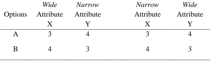
persons, A and B, on two attributes, X and Y (Wedell, 1998). He manipulated the ranges of the values along X and Y in two different ways. In the “wide-narrow” case, dimension X had a wide range of values and dimension Y had a narrow range; in the “narrow-wide” case, the opposite was true. Wedell measured the decision weights by subjective ratings of importance. He showed that these ratings were always greater for the dimension with the wider range, i.e. X in the wide-narrow condition and Y in the narrow-wide condition.
Table 3.1. A choice between two non-dominant options in two range conditions.
Wide Narrow Narrow Wide
Options Attribute X
Attribute Y
Attribute X
Attribute Y
A 3 4 3 4
B 4 3 4 3
Evidence that assessments depend on both dimensional similarity (which determines the subjective values of A and B on each attribute) and range similarity (which determines the decision weights of the attributes) comes from the observation that the global assessments were consistent with the prediction of the dimensional similarity but contradicted those of the range similarity. That is, in both narrow-wide and wide-narrow contexts, participants preferred the options that performed worse on the attribute they had rated as more important, i.e. A in the wide-range context and B
3.3 Implications for time preferences
Viewing interval as reflecting perceived temporal similarity between the outcomes provides insights into findings including the interval effect on outcome integrity, the notion of time contraction, and the “similarity effect” on time preferences, as we see next.
3.3.1 Integrity
Chapter 2 introduces the notion of integrity, which refers to the degree to which (discrete) outcomes are perceived as a whole (Loewenstein & Prelec, 1993)4. Example 2.3 shows that as the interval increases from one week to 26 weeks, the fraction of participants preferring the increasing (Aunt, Friends) is reduced by 38% (from 90% to 52%). That is, long intervals undermine integrity. From the current perspective, integrity implies the grouping of outcomes. Integrity is therefore a function of the perceived similarity between the outcomes. Long intervals signal lack of similarity and foster a shift in one‟s perceptions of the outcomes from being part of a group (sequence) to being isolated. Positive time preference dominates the assessments of isolated outcomes. Therefore, long intervals undermine preference for improvement.
While the visits are of the same kind, similar findings exist for outcomes that, on the face value, share little in common. For instance, Dhar and Simonson‟s (1999)
consumption episode effects refer to the finding that decision makers apply specific decision strategies to diverse outcomes, e.g. watching an opera and having a meal, that is, as long as these outcomes are perceived as constituting a consumption episode, e.g. an evening out. For instance, consumers facing tradeoffs between goal attributes
4
and mean attributes would choose to highlight goal achievements by sacrificing means. In one of their experiments, participants preferred an expensive meal to a moderately priced one when the meal took place immediately after an opera but not after a relatively cheap movie. They did this presumably to maximize the pleasure of the evening out. However, the highlighting strategy was not observed when the meal took place one week after the opera. From the current perspective, despite that watching an opera and having a meal shares little in common, they form an ad hoc
category that is specific to the decision context and the goals. Similar to what happens in natural categories, however, long intervals disrupt integrity in ad hoc categories as well.
Since delay does not reflect temporal similarity, it is no surprise that delay has little impact on outcome integrity. In Example 2.3, as the schedules were delayed by 26 weeks, the percentage of participants preferring (Aunt, Friends) was reduced only by 7% (from 90% to 83%). However, why did sequence preferences change with delay at all? Loewenstein and Prelec (1993) explained that longer delay fostered greater discounting, which reduced the attractiveness of the improving schedule that placed the more desirable event (visiting friends) later rather than earlier.
shorter than it actually is (Parducci, 1965, 1995). In either case, the role of intervals in separating outcomes from each other might be suspended.
A non-linear relationship between integrity and the perception of sequences, as well as between integrity and preference for improvement, emerges from this discussion. Outcomes that form a sequence need to be perceived as a whole and also as individuals. That is, they can neither be too integral nor too separate. Preference for improvement is undermined whether the integrity is too high or too low.
3.3.2 Time contraction
Time contraction means decision makers compress time and treat long intervals as if they were short (Read & Loewenstein, 1995). The range effect (Parducci, 1965, 1995) predicts that delay fosters time contraction. This is because delaying outcomes entails a larger range of time. This enhances perceived similarity in terms of time and decreases the perceived length of interval.
3.3.3 The “similarity effect”
Rubinstein obtained a finding, the similarity effect, which illustrates how time preferences depend on the range of attributes under consideration. Rubinstein (2003, Experiment III) showed participants the following two options:
A. In 60 days you are supposed to receive a new stereo system. Upon receipt of the system, you must pay $960. Are you willing to delay the transaction by one day for a discount of $2?
B. Tomorrow you are supposed to receive a new stereo system. Upon receipt of the system, you must pay $1,080. Are you willing to delay the delivery and the payment by 60 days for a discount of $120?
Hyperbolic discounting entails a discount rate that decreases with delay length. It predicts a preference for Option A over Option B because outcomes that offer a fixed rate of trade-off between money and time (i.e. $2 per day) are more attractive if the trade-off is more distant. In reality, most participants responded positively to B but not to A. One reason might be that the $2 saving in A was made trivial by the wider range of money ($120) in B (Parducci, 1965, 1995). However if $2 was perceived trivial even without the extended range (Gourville, 1998), then as Rubinstein argued, it was the similarity between the two payments in A that made the waiting of an additional day less worthwhile, a finding he called the similarity effect
the same, i.e. 60 days, in both options. Time may also be normalized to provide the basis for assessments (Ariely & Loewenstein, 2000).
3.3.4 Assessment mode
It is worth noting that the integrated and segregated modes represent two extreme ways of assessment. They can be viewed as defining the end-points of a continuous scale of assessment modes – the higher the integrity, the more likely the integrated mode, whereas the lower the integrity, the more likely the segregated mode. Sequence assessments represent an intermediate case, where both the values of the individual outcomes and their interactions exert influences. This is consistent with the view that sequence outcomes are both integral as a group and separate as individuals.
3.4 Relatedness
remained over half (54%) even when the interval was as long as 26 weeks (or 6 months). Without relatedness, this result would have seemed odd as the interval is so long that the participants should have exhibited an overwhelming preference for the decreasing (Friends, Aunt). From the current perspective, the integrity is retained because the outcomes happen in the same domain and assessed at the same time
This highlights the malleability of relatedness judgments. That is, as similarity, relatedness could arise naturally or in response to the decision context. It follows that two apparently unrelated outcomes can become related given appropriate contexts. For instance, making plans for “things to do during the weekends” encompasses both “cleaning the flat” and “reading one‟s favourite novel”. As a result, decision makers are more likely to choose to read the novel after the cleaning than the other way around. Likewise, an opera and a meal seem unrelated. However, endowed with episode-specific relatedness, one‟s decisions about the two are bounded by the desire to maximize the enjoyment of the episode (Dhar & Simonson, 1999).
3.5 Summary
Chapter 4
CONTEXT EFFECTS
4.0 Introduction
Tversky and Griffin (1991) posit that a past