Gradually varied open channel flow profiles normalized by critical depth and analytically solved by using Gaussian hypergeometric functions

(1)

Hydrol. Earth Syst. Sci., 17, 973–987, 2013 www.hydrol-earth-syst-sci.net/17/973/2013/ doi:10.5194/hess-17-973-2013

EGU Journal Logos (RGB)

Advances in

Geosciences

Open Access

Natural Hazards

and Earth System

Sciences

Open Access

Annales

Geophysicae

Open Access

Nonlinear Processes

in Geophysics

Open Access

Atmospheric

Chemistry

and Physics

Open Access

Atmospheric

Chemistry

and Physics

Open Access

Discussions

Atmospheric

Measurement

Techniques

Open Access

Atmospheric

Measurement

Techniques

Open Access

Discussions

Biogeosciences

Open Access Open Access

Biogeosciences

Discussions

Climate

of the Past

Climate

of the Past

Discussions

Earth System

Dynamics

Earth System

Dynamics

Discussions

Geoscientific

Instrumentation

Methods and

Data Systems

Open Access

_{Geoscientific}

Instrumentation

Methods and

Data Systems

Open Access

Discussions

Geoscientific

Model Development

Geoscientific

Model Development

Discussions

Hydrology and

Earth System

Sciences

Open Access

Hydrology and

Earth System

Sciences

Open Access

Discussions

Ocean Science

Discussions

Solid Earth

Discussions

The Cryosphere

Discussions

Natural Hazards

and Earth System

Sciences

Open Access

Discussions

Gradually varied open-channel flow profiles normalized by critical

depth and analytically solved by using Gaussian hypergeometric

functions

C.-D. Jan1and C.-L. Chen2, †

1_{Department of Hydraulic and Ocean Engineering, National Cheng Kung University, Tainan 70101, Taiwan} 2_{Consulting Hydrologist, Cupertino, California, USA}

†_Deceased

Correspondence to: C.-D. Jan ([email protected])

Received: 18 September 2012 – Published in Hydrol. Earth Syst. Sci. Discuss.: 17 October 2012 Revised: 4 February 2013 – Accepted: 9 February 2013 – Published: 5 March 2013

Abstract. The equation of one-dimensional gradually varied

flow (GVF) in sustaining and non-sustaining open channels is normalized using the critical depth,yc, and then

analyt-ically solved by the direct integration method with the use of the Gaussian hypergeometric function (GHF). The GHF-based solution so obtained from theyc-based dimensionless

GVF equation is more useful and versatile than its counter-part from the GVF equation normalized by the normal depth,

yn, because the GHF-based solutions of theyc-based

dimen-sionless GVF equation for the mild (M) and adverse (A) pro-files can asymptotically reduce to theyc-based dimensionless

horizontal (H) profiles asyc/yn→0. An in-depth analysis of

theyc-based dimensionless profiles expressed in terms of the

GHF for GVF in sustaining and adverse wide channels has been conducted to discuss the effects ofyc/yn and the

hy-draulic exponentN on the profiles. This paper has laid the foundation to compute at one sweep theyc-based

dimension-less GVF profiles in a series of sustaining and adverse chan-nels, which have horizontal slopes sandwiched in between them, by using the GHF-based solutions.

1 Introduction

Many hydraulic engineering works involve the computation of surface profiles of gradually varied flow (GVF) that is a steady non-uniform flow in an open channel with grad-ual changes in its water surface elevation. The computation methods of GVF profiles in open channels have been dis-cussed in many textbooks and journal papers (Chow, 1959;

Subramanya, 2009; Jan and Chen, 2012; Vatankhah, 2012). The most widely used methods for computing GVF profiles could be classified into the step methods and the direct in-tegration methods. The step methods are numerical methods and are primarily used in natural channels with non-prismatic sections. On the other hand, the direct integration methods involve the integration of the GVF equation and may be performed by using analytical, semi-analytical, or numeri-cal procedures. Numerinumeri-cal integration of the GVF equation is primarily used in non-prismatic channels. In some prismatic channels, such as artificial channels, the GVF equation can be simplified so as to let the analytical (or semi-analytical) di-rect integration be applied. The analytical didi-rect-integration method is straightforward and can provide the total length of the profile in a single computation step. In the direct-integration method, the one-dimensional (1-D) GVF equa-tion is usually normalized to be a simpler expression in ad-vance so as to allow the performance of direct integration. In most cases, the GVF equation is normalized by the normal depth yn (Chow, 1959; Subramanya, 2009; Jan and Chen,

2012; Venutelli, 2004; Vatankhah, 2012), while in some cases, it is normalized by the critical depth yc (Chen and

(2)

974 C.-D. Jan and C.-L. Chen: Gaussian hypergeometric functions

to analytically solve the GVF equation in sustaining wide channels without recourse to the VFF.

Success to formulate the normal-depth(yn)-based

non-dimensional GVF profiles expressed in terms of GHFs for flow in sustaining channels, as reported by Jan and Chen (2012), does not necessarily warrant that it can likewise prevail to useynin the normalization of the GVF equation for

flow in adverse channels becauseynfor an assumed uniform

flow in adverse channels is undefined. Even though one can use an imaginary flow resistance coefficient to evaluateynfor

such an assumed uniform flow in adverse channels (Chow, 1959), as will be treated later in this paper, it is inappropriate to use such anynin the normalization of the GVF equation

for flow in adverse channels becauseynso evaluated is

ficti-tious and the two normalized variables in suchyn-based

di-mensionless GVF equation collapse (in virtue ofyn→ ∞)

as the channel-bottom slope approaches zero. To fill such a mathematical gap as a result of the indiscreet choice of a characteristic length in the normalization of the GVF equa-tion for adverse channels, Chen and Wang (1969) usedycto

replaceynalong to derive twoyc-based dimensionless GVF

equations, one for sustaining channels and the other for ad-verse channels. For the hydraulic exponents M=3 (wide channels) andN=10/3 (equivalent to using Manning’s for-mula) they integrated both equations numerically over the normalized depth, y/yc, to get the yc-based dimensionless

GVF profiles in sustaining and adverse channels.

This study focuses on the direct integration method that used to analytically compute the GVF profiles in sustaining and non-sustaining channels, in which the GVF equation is normalized by usingycand then analytically solved by using

the GHFs. Before proceeding to formulate the twoyc-based

dimensionless GVF equations for sustaining channels and adverse channels, respectively, it is worthwhile to review all of what has been attained by previous investigators to com-pute the GVF profiles in both sustaining and adverse chan-nels. We already reviewed quite comprehensively most of the previous work on the analytical computation of the GVF pro-files in sustaining channels, as reported in our paper (Jan and Chen, 2012). Therefore, in this paper, we focus on the liter-ature survey only of the computed GVF profiles in adverse channels.

As a matter of fact, there are not many previous investi-gators who have contributed to the computation of the GVF profiles in adverse channels. One of the earliest investiga-tions in this study may be credited to Matzke (1937), who formulated the yn-based dimensionless GVF equation for

GVF in adverse channels, thereby integrating the indefinite integrals of the GVF equation in the form of the varied-flow function (VFF), following in Bakhmeteff’s (1932) foot-steps. However, unlike the four methods used by Bakhmeteff to compute the VFF values numerically, Matzke evaluated them by a graphical method and constructed a table thereof for any N values between 3 and 4, inclusive, for computing the yn-based dimensionless GVF profiles in adverse

chan-nels. Chow (1957, 1959) was probably the first person who directly computed the VFF values for GVF in adverse chan-nels from the corresponding two transformed VFF values for GVF in sustaining channels. He further tabulated the VFF values so computed for N values ranging from 3 to 5.5 for use in engineering applications to compute theyn-based

di-mensionless GVF profiles in adverse channels.

In the direct integration of the GVF equation, regardless of whether it is carried out for sustaining or adverse chan-nels, most previous investigators expressed the rational func-tion representing the reciprocal of the slope of the GVF pro-file in terms of the dimensionless flow depth rather than in terms of the geometric elements of a given channel section before the two indefinite integrals were evaluated. Never-theless, Allen and Enever (1968) as well as Kumar (1979) did it in reverse by substituting their geometric elements of a rectangular, trapezoidal, or triangular channel section into the section factor,Z, and the conveyance,K, of the channel section in the GVF equation before evaluating the two inite integrals. Subsequently, they evaluated the two indef-inite integrals using the partial-fraction expansion and then got the elementary-transcendental-function (ETF)-based so-lution for each of the cross-sectional shapes under study, such as rectangular, triangular and parabolic cross-sectional shapes. Another approach taken by Zaghloul (1990, 1992) to integrate the GVF equation for the profiles in circular pipes was the same as that used by Allen and Enever (1968) by substituting the geometric elements of a circular conduit sec-tion intoZandKin the GVF equation before integrating it by use of Simpson’s rule (Zaghloul, 1990) or both the direct step and integration methods (Zaghloul, 1992). After all, he developed a computer model on the basis of such methods to compute GVF profiles not only in sustaining and horizontal pipes, but also in adverse pipes.

For computing GVF profiles in sustaining channels, one can solve theyn-based dimensionless GVF equation by using

the direct integration method and the Gaussian hypergeomet-ric function (GHF), as presented by Jan and Chen (2012). Nevertheless, for computing GVF profiles in adverse chan-nels, one cannot do likewise due to the difficulty in quan-tifying theyn-value to be used in the normalization of the

GVF equation becauseyn for an assumed uniform flow in

adverse channels is undefined. Use of yc instead of yn in

the normalization of the GVF equation for flow in adverse channels can resolve such a vital issue resulting from the undefinedyn because yc can be uniquely determined for a

given discharge. The primary objective of this paper is thus to formulate and then analytically solve the twoyc-based

di-mensionless GVF equations for GVFs in both sustaining and adverse channels by using the direct integration method and the Gaussian hypergeometric functions (GHFs). The GHF-based solutions of this study will lay the theoretical founda-tion to compute suchyc-based dimensionless GVF profiles in

(3)

2 Critical-depth-based dimensionless GVF equations

Before deriving theyc-based dimensionless one dimensional

GVF profiles in sustaining channels (S0>0), horizontal

channels (S0=0), and adverse channels (S0<0), we first

formulate the yc-based dimensionless GVF equations for

three such types of channels in the following.

2.1 Equation of the GVF in sustaining channels

The dimensional form of the 1-D GVF equation expressed in terms of the flow depth prior to normalization can be written as (Chow, 1959)

dy

dx =S0

1−(yn/y)N

1−(yc/y)M

. (1)

This equation is a first order differential equation and denotes the relation between the flow depthyand the axial distancex

along the open channel having a slopeS0. The subscripts “n”

and “c” refer to the normal and critical flow conditions, re-spectively. The exponentsMandNare usually called the hy-draulic exponents for critical-flow computation and uniform-flow computation, respectively. It is expected that the solu-tion of Eq. (1), if obtainable, can be expressed in a form of

y as an implicit function ofx withS0,yn,yc,M, andN as

parameters.

Though the validity of Eq. (1) is not at issue, one should be aware of its implication before normalizing it for solu-tion. Firstly, the resistance to GVF in open channels, as in-corporated in Eq. (1), is conventionally evaluated on the as-sumption that the resistance at any section is equal to what it would be as if the sameQpassed through the same sec-tion under condisec-tions of uniformity. However, this conven-tional assumption made in Eq. (1) does not take the effect of boundary non-uniformity into account in the evaluation of the non-uniform flow resistance. According to Rouse (1965), the effect of boundary non-uniformity on the flow resistance should include any change in shape or size of the section along the longitudinal direction. Secondly, Eq. (1) cannot be used to compute GVF profiles in nonsustaining (horizontal or adverse) channels becauseynis infinite for flow in

hori-zontal channels and undefined for flow in adverse channels. Thirdly,N is related to the power in the power-law flow re-sistance formula, which has been incorporated in formulating Eq. (1). It is noted thatN=3 for hydraulically smooth flows andN=2m+3 (wheremis the exponent of a unified sim-ilarity variable used in the power laws of the wall) for fully rough flows (Chen, 1991).

By and large, there are two ways in whichx and y in Eq. (1) can be normalized: one is based on the normal depth,

yn, as usually adopted by many researchers (Chow, 1959)

for GVF in sustaining channels, and the other based on the critical depth,yc, as treated by Chen and Wang (1969), who

adoptedycin place ofynto compute in one sweep GVF

pro-files in a series of interconnected sustaining and

nonsustain-ing channels. Therefore, for the first case in which Eq. (1) is normalized based on yn, we can introduce the

dimen-sionless variablesu(=y/yn)andx∗(=xS0/yn), as done by

Chow (1959), Jan and Chen (2012) among others, thereby expressing the reciprocal of Eq. (1) in terms ofuandx∗as

dx∗

du =

−uN+λMuN−M

1−uN (2)

which has been referred to as the dimensionless GVF equa-tion based onynwithλ(=yc/yn),M, andNas three

param-eters. The characteristic length ratioλin Eq. (2) is the pri-mary parameter that classifies the GVF profiles into those in the mild (M), critical (C), and steep (S) channels if the ratio

λis less than, equal to, and larger than unity, respectively. Instead ofyn, we want to useyc to normalizex andy in

Eq. (1) herein by simply adopting the dimensionless vari-ablesv (=y/yc)andx# (=xSc/yc), as done by Chen and

Wang (1969), to rewrite the reciprocal of Eq. (1) in terms of

vandx#so as to obtain the followingyc-based dimensionless

GVF equation withλ,M, andN as three parameters. dx#

dv =

−vN+vN−M

1−(λv)N (3)

which is valid in the domain of 0≤v <∞.

The following two relations are the normalized flow depth and normalized longitudinal coordinate defined on the basis ofynto their counterparts defined on the basis ofyc:

u v =

yc

yn

(4)

x∗

x#

=yc yn

S0

Sc

= _y

c

yn

N+1

. (5)

Both normalized variables so related in Eqs. (4) and (5) will be useful in converting the solutions of Eq. (2) to its counter-parts obtained from Eq. (3), or vice versa.

2.2 Equation of the GVF in horizontal channels

Although Chow (1959, p. 223) did not classify horizontal channels as a type of sustaining channels, we can prove that theyc-based dimensionless GVF equation, Eq. (3), is

still valid for GVF profiles in horizontal channels. In other words, because we haveS0=0,yn→ ∞, andλ(=yc/yn)→

0 for GVF profiles in horizontal channels, Eq. (3) can be simplified to

dx#

dv =v

N−M₋_vN ₍₆₎

which is still valid in the domain of 0≤v <∞. Equation (6) is the dimensionless equation based onyc for GVF profiles

(4)

N, Eq. (3) can be analytically integrated over v using the GHF, as will be shown later, while we can directly integrate Eq. (6) without resorting to the GHF in the following manner.

x#=

vN−M+1 N−M+1−

vN+1

N+1+Const (7)

The above equation describes the yc-based dimensionless

GVF profiles in wide horizontal channels (in whichM=3). The constant of integration, “Const”, in Eq. (7) is to be deter-mined from a given boundary condition. It should be noted that Eq. (7) can readily be identified with Chow’s (1959, Sect. 10.2) Eqs. (10)–(26).

Chow’s (1959, Sect. 10.2) classification to distinguish a horizontal slope (S0=0) from a sustaining slope (S0>0)

or an adverse slope (S0<0) seems at odds with the limit

of differential calculus, because theyc-based dimensionless

horizontal profiles, Eq. (7), can be derived from theyc-based

dimensionless equation for GVF profiles in sustaining or ad-verse channels having any realS0-values. In fact, Chow could

have treated GVF profiles on a horizontal slope as the asymp-tote of those on a sustaining slope as S0→0, as deduced

above from Eqs. (3) to (7) by lettingλ→0 (oryn→ ∞). We

shall also later prove that the GHF-based solutions of Eq. (3) for GVF on the mild slope (where 0< λ <1) can reduce to Eq. (7) when we approach its asymptote by lettingλ→0. Likewise, theyc-based dimensionless equation for GVF in

adverse channels, as will be formulated later, can also ap-proach its asymptote, namely Eq. (7), asλ→0. Therefore, for coherence in treating the asymptote of theyc-based

di-mensionless GVF equation and its solutions throughout the paper, we henceforth regard the horizontal slope as an inter-mediate (or interface) between the sustaining slope and the adverse slope asS0approaches zero from either slope. 2.3 Equation of the GVF in adverse channels

To formulate theyc-based dimensionless GVF equation for

GVF in adverse channels, we deem the slope of the channel bottom as negative, i.e.S0<0. Such a fictitious treatment

may result in an imaginary value ofKn(the conveyance for

uniform flow at a depthyn)or a negative value ofKn2for a

givenQ(=KnS₀q, providedq=1/2). Althoughynfor

uni-form flow in adverse channels is undefined, we may assume that the coefficient of the flow resistance,C, in the flow resis-tance formula is imaginary so as to enable the computation ofyn. In other words, for a negative value ofKn2, the value of

C2used in computingyn fromKn2=C2A2nR 2p

n (where pis

the exponent related to the flow resistance formula;p=2/3 for Manning’s formula andp=1/2 for Ch´ezy formula) must be negative, thus resulting in a fictitious value ofyn, if

deter-mined from the above relation. Because the critical depthyc

can be determined from the critical relation for a givenQ

(Chow, 1959, Sect. 4.2), the fictitiousynso calculated can be

further incorporated withycto derive the followingyc-based

dimensionless equation for GVF in adverse channels. dx#

dv =

−vN+vN−M

1+(λv)N (8)

in whichv=y/ycandx#=xSc/yc, the same dimensionless

variables used in the derivation of Eq. (3). As pointed out ear-lier, Eq. (8) for GVF in adverse channels can reduce asymp-totically to Eq. (6) for GVF in horizontal channels asS0→0

(i.e.yn→ ∞orλ→0).

Undoubtedly, at issue herein is the controversial approach taken in evaluatingyn for use in Eq. (8) because the

resis-tance coefficient in the flow resisresis-tance formula is assumed to be imaginary and theyn-value so evaluated is fictitious in an

adverse channel. Nevertheless, for a givenQ, theyc-value so

computed is unique, regardless of whether it is in a sustaining or adverse channel. The parameter,λN, appearing in Eq. (8) signifies the slope ratio,So/Sc, thus implying thatλN is of a

negative value for GVF in adverse (S0<0) channels.

There-fore, λ (=(S0/Sc)1/N) as a parameter for GVF in adverse

channels is not so physically meaningful as that in Eq. (3) for GVF in sustaining channels, in which the flow criteria of theλ-value being less than, equal to, and greater than unity can represent respectively the GVF on the mild, critical, and steep slopes. In contrast, the fictitiousλ-value in Eq. (8) for GVF in adverse channels is nothing but an index. Although the ultimate usefulness of Eq. (8) may not be realized un-til after such an issue in the evaluation ofynis resolved, we

presently rest content with such fictitiousyn because there

appears no other approach better than that taken above to evaluateynfor GVF in adverse channels.

Althoughyn-value so evaluated is fictitious in an adverse

channel regardless of whether Eq. (1) is normalized on the basis ofyc oryn, we prefer to normalize Eq. (1) based on

yc rather than based on yn for the following main reason.

Most previous investigators, such as Chow (1957, 1959) for-mulated theyn-based dimensionless GVF equation for

com-puting GVF profiles in adverse channels, i.e., theyn-based

counterpart of Eq. (8) instead of theyc-based Eq. (8).

How-ever, Eq. (8) has the obvious advantage over its yn-based

counterpart because the latter cannot reduce asymptotically to Eq. (6) asS0→0 (i.e.yn→ ∞orλ→0) unless the

nor-malizing quantity of theyn-based GVF equation for adverse

channels can be altered from yn toyc so as to enable one

to switch the normalized variables fromutov via Eq. (4) and fromx∗ tox#via Eq. (5) asS0→0. By implication, if

the yn-based counterpart of Eq. (8) would have been used

to compute GVF profiles in adverse channels, the horizontal slope could not have been treated as an intermediate (or in-terface) between the sustaining slope and the adverse slope asS0→0. Insomuch that, we can deem Eq. (8) with the

pa-rameter,λ, a completely general equation to compute theyc

(5)

3 Gaussian hypergeometric function

Prior to find the analytical solutions of the critical-depth-based equations for the gradually varied flows in sustaining and adverse channels by using the Gaussian hypergeometric function (GHF), we will introduce the definition of GHF and some relations first. GHF can be expressed as an infinite se-ries and symbolized in the form of2F1(a,b;c;z)as shown

in the books of Korn and Korn (1961), Luke (1975), Pear-son (1974), and Seaborn (1991). The form2F1(a, b; c; z)

can be safely changed to the more friendly formF (a,b;c;

z)as Olde Daalhuis (2010, Sect. 15.1) indicates, i.e.

F (a, b;c;z)= 0(c) 0(a)0(b)

∞

X s=0

0(a+s)0(b+s) 0(c+s)s! z

s ₍₉₎

in which a, b, and c are the function parameters and z is the variable. The infinite series in Eq. (9) is convergent for arbitrary a, b, and c, provided that c is neither a negative integer nor zero and that a or b is not a negative integer for real−1< z <1 (or|z|<1), and forz= ±1 ifc > a+b

(Olde Daalhuis, 2010). Equation (9) has the symmetric prop-erty:F (a,b;c;z)=F (b,a;c;z).

A survey of the literature reveals that there are two lin-early independent solutions of the hypergeometric differen-tial equation at each of the three singular pointsz=0, 1, and

∞for a total of six special solutions, which are in fact fun-damental to Kummer’s (1836) 24 solutions. Any three of the aforementioned six special solutions satisfy a relation, thus giving rise to twenty combinations thereof. Among them, there is a relation connecting one GHF in the domain of

|z|<1 to two GHFs in the domain of|z|>1 in the following way (Luke, 1975):

F (a, b;c;z)=0 (b−a) 0 (c) 0 (b) 0 (c−a)

−z−1a

Fa, a−c+1;a−b+1;z−1+0 (a−b) 0 (c) 0 (a) 0 (c−b)

−z−1b

Fb, b−c+1; −a+b+1;z−1

. (10)

One may use Eq. (10) to transform the GHF-based solu-tions in the domain of |z|<1 to their counterparts in the domain of |z|>1. The commercial Mathematica software treats Eq. (10) as a definition ofF (a,b;c;z)for|z|>1 (Wol-fram, 1996).

For the special case,a,b, andcare fixed with specified relations,a=1 andc=b+1, Eq. (9) can be written as

F (1, b;b+1;z)=g(b, z)=b

∞

X s=0

zs

b+s. (11)

The GHFs used in the solutions of the gradually varied flow profiles herein are all in the form of Eq. (11). Since the first argument of the GHF of Eq. (11) is always unity, the second and third arguments differ in one unity, and the fourth argu-ment is a variable only, we can express the GHF in a simpler

expression, such asg(b,z)=F(1,b;b+1;z), to reduce the related equations to shorter expressions for facilitating the reading of the manuscript, as treated by Jan and Chen (2012). Therefore, we will use g(b,z) instead of F(1, b; b+1;z)

herein to represent GHF when we treat the GHF-solutions in the present paper.

The following recurrence formulas between two GHFs can be generally established from Eq. (11) as shown in Jan and Chen (2012).

g (b, z)=1+ bz

b+1g (b+1, z) . (12) Since 0(b)= (b−1)0(b−1), 0(b+1) = b0(b), and F

(b,0;b;z−1)=1, we can rewrite Eq. (10), for |z|>1, in a much shorter expression as

g (b, z)= −bz

−1

b−1g

1−b, z−1 +0 (1−b) 0 (1+b)

−z−1

b

. (13)

In addition, for the condition (βt )N<1 (i.e. βt <1) , in whichβ is a positive parameter,t is a positive variable, and

N is a positive real number, using the commercial

Mathe-matica software (Wolfram, 1996), we can find the following

general relation for the solution of the indefinite integral in terms of GHF as shown below.

Z _tφ

1∓(βt )Ndt= tφ+1 φ+1g

_φ₊₁

N , ±(βt ) N

+Const (14) in which the parameter φ is a real number. The term (βt )

in Eq. (14) could be (λv)or (w/λ)for the study herein as shown in the next sections. This kind of indefinite integrals as shown in Eq. (14) will be applied many times in the following sections when we find GHF-based solutions for GVF profiles in sustaining and adverse channels.

4 Analytical solutions of theyc-based GVF equations

There are two ways to analytically solve the normal-depth-based (yn-based) dimensionless GVF equation by the

direct-integration method: One is based on the GHF and the other on the elementary transcendental functions (ETF). The inno-vative results obtained by Jan and Chen (2012) shows that the GHF-based solutions are more useful and versatile than the ETF-based solutions, because the former allows its involved parametersMandNbeing real numbers while the latter can at the most accept rational numbers, but not real numbers. This paper is henceforth focused only on the acquisition and analysis of the GHF-based solutions for the critical-depth-based (yc-based) dimensionless GVF equation. Analogous

to the direct integration of theyn-based dimensionless GVF

(6)

4.1 Alternative forms of Eqs. (3) and (8)

The validity of the solutions of Eq. (3) or (8) to be expressed in terms of the GHF is confined to the convergence criterion of GHF itself, i.e.|λv|<1. Therefore, an alternative form of Eq. (3) or (8) has to be formulated so as to allow its solu-tions expressed in terms of the GHF be valid for|λv|>1. Every GHF-based solution of Eq. (3) or (8) thus consists of two parts: one in the domain of|λv|<1 and the other in the domain of|λv|>1. To derive alternative forms of Eqs. (3) and (8) in order that their GHF-based solutions be valid for

|λv|>1, Eqs. (3) and (8) on substitution ofv=w−1and dv

= −w−2dw will respectively yield the following Eqs. (15) and (16) for GVF in sustaining and adverse channels, respec-tively.

dx#

dw =λ

−N−w−2+wM−2

1−(w/λ)N (15)

dx#

dw =λ

−Nw−2−wM−2

1+(w/λ)N (16)

Before procuring the GHF-based solutions from Eqs. (15) and (16), it merits mentioning that such GHF-based solu-tions, if obtainable, are premised on the assumption that they are valid only in the domains of|w/λ|<1 (i.e.|λv|>1).

4.2 GVF profiles in sustaining channels

For facilitating the direct integration to obtain the GHF-based solutions of Eq. (3) for|λv|<1 and Eq. (14) for|λv|>1, we can rearrange Eq. (3) into three different forms. The right-hand side of Eq. (3) is the rational function ofv, which by the process of long division can be expressed in the form of a polynomial plus a proper fraction in two ways before we integrate them. One way is to divide the first term of the nu-merator on the right-hand side of Eq. (3) by the denominator; the other way is to divide the second term of the numerator on the right-hand side of Eq. (3) by the denominator. There-fore, they are three possible representations of the solution of Eq. (3) by the direct integration method, as shown below.

x#= −

Z _vN

1−(λv)Ndv+

Z _vN−M

1−(λv)Ndv+Const (17)

x#=

vN−M+1 N−M+1−

Z _vN

1−(λv)Ndv+λ N

Z _v2N−M

x#= −

vN+1 N+1+

Z _vN−M

1−(λv)Ndv−λ N

Z _v2N

The GHF-based solutions for Eqs. (17), (18) and (19) can be easily obtained by using the help of Eq. (14). Three GHF-based solutions to be obtained from Eq. (17) to Eq. (19) should be identical. Equating any two of the three GHF-based solutions will thus establish a recurrence formula be-tween the two contiguous GHFs as shown in Eq. (12). Only one of the three solutions is needed. Because Eq. (17) has shorter length of expression, we will use it latter to derive our GHF-based solutions for GVF profile in a sustaining channel. Likewise, to derive the GHF-based solutions of Eq. (15) for|λv|>1, we can make a direct integration to Eq. (15) as shown below.

x#= −λ−N

Z _w−2

1−(w/λ)Ndw+λ

−N

Z _wM−2

1−(w/λ)Ndw+Const (20)

With the help of Eq. (14), the complete GHF-based solutions of the dimensionless GVF equation, Eq. (3), for GVF in sus-taining channels can be obtained by executing the integra-tion of the two indefinite integrals in Eq. (17) for |λv|<1 and then carrying out the same in Eq. (20) for|w/λ|<1 (or

|λv|>1), as shown below.

x#= −

vN+1 N+1g

_N₊₁ N , (λv)

N

+ v N−M+1

N−M+1g

_N₋_M₊₁ N , (λv)

N₊_Const ₍₂₁₎

which is valid only for|λv|<1.

x#=λ−Nw−1g

₋₁ N ,

w λ

N +λ

−N_wM−1

M−1 g

_M₋₁ N ,

w λ

N

+Const (22)

which is valid only for |w/λ |<1. To express Eq. (22) in terms ofv, we substitutew=v−1into Eq. (22) to have

x#=λ−Nvg

−1

N, (λv)

−N

+λ

−N_v−M+1

M−1 g

M−1

N , (λv)

−N

+Const (23)

which is valid only for|λv|>1.

It is worthwhile to reiterate that we can use Eq. (13) to transform the GHF-based solutions in the domain of|z|<1 to their counterparts in the domain of|z|>1. Herez=(λv)N

(7)

It should be noted that such GHF-based solutions exclude points where|λv|=1 (or|w/λ|=1) because the GHF diverges at|λv|=1 (or|w/λ| =1). Physically, such points correspond to the convergent limits of the GHF in the GHF-based solu-tions of Eq. (3) atx#= ∞, where GVF profiles run parallel

with the channel bottom.

Although the absolute value of the variable in the GHF, i.e.|(λv)|, has been imposed to derive the GHF-based solu-tions of Eq. (3) for GVF profiles in sustaining channels, the complete GHF-based solutions of Eq. (3) can only cover the physically possible domain ofλv, i.e. 0≤λv <∞, thus con-sisting of Eq. (21) for 0≤λv <1, x#= ∞ atλv=1, and

Eq. (23) forλv >1. Insomuch that we can lift the absolute-value restriction imposed onλvin expressing the GHF-based solutions without the loss of generality.

4.3 GVF profiles in adverse channels

By the same token, the solution of the GVF profiles in ad-verse channels by the direct integration method can be ob-tained from Eq. (8) for|λv|<1 and Eq. (16) for |λw|<1 (i.e.|λv|>1), as shown below.

x#= −

Z _vN

1+(λv)Ndv+

Z _vN−M

1+(λv)Ndv+Const (24)

x#=λ−N

Z _w−2

1+(w/λ)Ndw−λ

−N

Z _wM−2

1+(w/λ)Ndw+Const (25)

With the help of Eq. (14), the complete GHF-based solutions of Eq. (8) for dimensionless GVF profiles in adverse chan-nels can be obtained by executing the integration of the two indefinite integrals in Eq. (24) for|λv|<1 and then carry-ing out the same in Eq. (25) for|w/λ|<1 (or|λv|>1). The results are

x#= −

vN+1 N+1g

_N₊₁ N ,−(λv)

N

+ v N−M+1

N−M+1g

_N₋_M₊₁ N ,−(λv)

N

+Const (26)

x#= −λ−Nw−1g

−1

N,− w

λ N

−λ

−N_wM−1

M−1 g

M−1

N ,− w

λ N

+Const. (27)

Equations (26) and (27) should be valid in the domain of

|λv|<1 and|w/λ|<1, respectively. To express Eq. (27) in terms ofv, substitutingw=v−1into Eq. (27) yields

x#= −λ−Nvg

−1

N,−(λv)

−N

−λ

−N_v−M+1

M−1 g

_M₋₁ N ,−(λv)

−N

+Const (28)

which is valid only for|λv|>1.

It is also found that the two GHFs appearing in each of Eqs. (26) and (28) converge but not diverge atλv=1 because the variable of both GHFs is of a negative value through its entire domain of λv≥ 0. That is to say that Eqs. (26) and (28) cover the domains of 0≤ λv≤1 andλv≥ 1, re-spectively. Although the absolute value of the variable in the GHF, i.e.|λv|, has been imposed to derive the GHF-based so-lutions from both Eqs. (8) and (16), the complete GHF-based solutions of Eq. (8) for GVF profiles in adverse channels can only cover the physically possible domain of λv≥0. It is thus inferred that the A1 profile does not exist.

It is worthwhile to reiterate that we can use Eq. (13) to transform the GHF-based solutions in the domain of

|z|<1 to their counterparts in the domain of |z|>1. Here

z=−(λv)N for Eq. (26). That is to say that we can use Eq. (13) to directly transform Eq. (26) to Eq. (28), and vice versa, without recourse to the formulation of Eq. (16) [i.e. an alternative form of Eq. (8) with its variable, w, being ex-pressed as v−1], which can be solved for GVF profiles in the domains of|w/λ|<1 (i.e.|λv|>1), thereby proving that we can obtain Eq. (28) directly from Eq. (26) rather than in-directly through Eq. (16), vice versa. If we accept Eq. (10) is a definition of GHF for |z|>1, as treated by the com-mercial Mathematica software (Wolfram, 1996), then one of Eqs. (26) and (28) is enough to represent the complete GHF-based solutions of Eq. (8) for GVF profiles in ad-verse channels, covering the physically possible domain of 0

≤λv <∞. Table 1 shows the summary of the critical-depth-based dimensionless GVF profiles expressed by using the GHF on all types of slopes.

5 Discussions

5.1 Plotting the GHF-based solutions withλas a parameter

Equations (21) and (23), which span respectively the do-mains of 0≤λv <1 and λv >1, are the GHF-based solu-tions of Eq. (3) foryc-based dimensionless GVF profiles in

sustaining channels, while Eqs. (26) and (28), covering re-spectively the domains of 0≤λv≤1 andλv≥1, are GHF-based solutions of Eq. (8) foryc-based dimensionless GVF

profiles in adverse channels. As explained in the last section, one of Eqs. (26) and (28) is enough to represent the com-plete GHF-based solutions of Eq. (8) for GVF profiles in ad-verse channels, covering the whole domain of 0≤λv <∞. Equation (26) is chosen herein. A plot of Eqs. (21), (23) and (26) on the (x#, v)-plane with λ as a parameter may

(8)

[image:8.595.53.283.61.369.2]

980 C.-D. Jan and C.-L. Chen: Gaussian hypergeometric functions Figure 1. A plot of the yc-based dimensionless 1-D GVF profiles for M = 3 and N =

10/3 with yc/yn as a parameter.

-15 -10 -5 0 5 10

x#

0 1 2 3 4 5 6 7 8 9 10

v

M1

yc/yn =0.9

1.1 M2

1.9 A2

0.3

1.1 1.7

0.8

S3

1.3 1.5 1.9 S1

C1

H2

0.7 0.6 0.5 0.4

0.3

0.4 0.5 0.6

0.7 0.8

0.9

0.3 0.4

0.5 0.6

0.7 0.8 0.9

1.3

1.5 1.7

S2 M3

H3 A3

C3 1.0

1.1 1.3

2.0 1.5

1.0 0.0

Fig. 1. A plot of theyc -based dimensionless 1-D GVF profiles for M=3 andN=10/3 withyc/ynas a parameter.

v)-plane herein, as shown in Fig. 1. In Fig. 1, three bound-ary conditions are arbitrarily prescribed at (x#,v)=(10,10)

for Eq. (23), and at (x#,v)=(0,0)for Eqs. (20) and (26),

respectively. There exist twelve types of theyc-based GVF

profiles, two on the H slope (λ=0), three on the M slope (0< λ<1), two on the C slope (λ=1), three on the S slope (1< λ <∞), and two on the A slope (0≤λ <∞, in which

yn is fictitious). The twelveyc-based GVF profiles in three

zones may be respectively referred to as H2 and H3; M1, M2, and M3; C1 and C3; S1, S2, and S3; A2 and A3. The twelve profiles so classified are the same as those classified by Chow (1959) except for C2 (Chow treated it as for a uni-form flow), which is excluded from our classification because it is just a singularity for all the N values except forN=3, as treated by Jan and Chen (2012).

5.2 Mild (M), steep (S), and adverse (A) profiles in zones 1, 2, and 3

Examination of Fig. 1 reveals that two solution curves drawn for the critical value ofλ(i.e.λ=yc/yn=1) and the

asymp-totic value of λ (i.e. λ=0) combined with the horizontal line at v=1 and the horizontal asymptotes at λv=1 (or

v=yn/yc)can divide the entire domain of the solution curves

on the (x#,v)-plane into nine regions, which are constituted

by a combination of three slopes and three zones, i.e. the same division adopted by Chow (1959). The three slopes consist of mild (M) slopes, steep (S) slopes, and adverse (A) slopes, while the three zones are composed of zone 1 (λ < v <∞for M1 profiles or 1≤v <∞ for S1 profiles), zone 2 (1≤v < λfor M2 profiles,λ < v≤1 for S2 profiles, or 1 ≤ v <∞ for A2 profiles), and zone 3 (0≤v≤1 for M3 profiles, 0≤v < λfor S3 profiles, or 0≤v≤1 for A3 profiles). Apparently, the particular solution curves drawn by Eqs. (21) and (23) withλ(=yc/yn)=1 separate the region of

M profiles from that of S profiles, while the unique solution curve constructed by Eq. (7) through the asymptotic reduc-tion of Eq. (21) or (26) asλ→0 separate the region of M profiles from that of A profiles. These two solution curves are respectively referred to as the critical (C) profiles on the critical (C) slope (λ=1) and the horizontal (H) profiles on the horizontal (H) slope (λ=0).

5.3 Critical (C) profiles in zones 1 and 3

The particular solutions of Eqs. (21) and (23) on substitution ofλ=1 yield

x#= −

vN+1 N+1g

_N₊₁ N , v

N

+ v N−M+1

N−M+1g

_N₋_M₊₁ N , v

N

+Const (29)

x#=v g

−1

N, v

−N

+v

−M+1

M−1 g

_M₋₁ N , v

−N

+Const (30)

which are specifically referred to as the equations for yc

-based C3 profiles in zone 3 (0≤v <1) and C1 profiles in zone 1 (1<v <∞), respectively. In particular, upon substi-tution ofM=N=3 and with the use of the recurrence for-mulas Eq. (12), Eq. (29) can readily reduce to

x#=v+Const (31)

[image:8.595.307.522.326.449.2]

(9)

C.-D. Jan and C.-L. Chen: Gaussian hypergeometric functions 981

-1 -0.5 0 0.5 1

x#

0 0.5 1 1.5 2

v

M2 A2

0.3

1.1

1.7 1.3

1.5

2.0 0.4 0.5

0.6 0.7 0.8

yc/yn = 1.5

0.3 0.4 0.5

0.6

0.7

0.8

0.9

S3 M3

A3

C3 1.3

1.1 1.0 0.9

2.0 3.0 5.0

1.0

5.0

10.0 3.0 H2

H3 0.0

Fig. 2. A close-up of those H, M, C, S and A profiles which are plotted in Fig. 1 around the boundary condition at (x#,v)=(0,0).

5.4 Horizontal (H) profiles in zones 2 and 3

To separate the region of M profiles from that of A profiles is a solution curve plotted by use of Eq. (7), to which Eqs. (21) and (26) reduce asymptotically asλ→0 from either side of Eq. (7), as shown in Fig. 1. For clarity in highlighting this line of demarcation, Eq. (7), i.e. a solution curve forλ=0, we draw Fig. 2, a close-up of Fig. 1 around the commonly pre-scribed boundary condition of Eqs. (7), (21) and (26) at (x#,

v)=(0,0). One can easily prove that Eq. (7) can be obtained by the asymptotic reduction of Eq. (21) or (26) asλ→0, us-ing the GHF definition. The A2 and A3 profiles plotted usus-ing Eq. (26) can also reduce asymptotically to Eq. (7) asλ→0. As displayed clearly in Fig. 2, the H2 profile divides per-fectly between the regions of M2 profiles and A2 profiles; so does the H3 profile between the regions of M3 profiles and A3 profiles.

5.5 Horizontal asymptotes atv=yn/ycfor various

λ-values

It is already known that Eqs. (21) and (23) diverge along the horizontal asymptotes. However, unlike the sole horizontal asymptote atu=1 on the (x∗,u)-plane to represent the water

surface running parallel with the channel bed asx∗→ ±∞,

as shown in the Fig. 1 of Jan and Chen (2012), the horizon-tal asymptotes atv=λ−1(i.e. λv=1) for variousλ-values on the (x#,v)-plane translate vertically, as shown in Fig. 1

herein. Accordingly, the horizontal asymptotes atv=λ−1on the (x#,v)-plane for the givenλ-values may be deemed as

“movable” lines of demarcation drawn to divide the domain ofvinto two major regions: One region spans 0≤λv <1 (or 0≤v < λ−1), which covers both zones 2 and 3 for M profiles as well as zone 3 for S profiles, and the other region extends overλv >1 (orv > λ−1), which covers zone 1 for M profiles as well as both zones 1 and 2 for S profiles.

In comparison, there exist no horizontal asymptotes at

v=λ−1 for various λ-values in the domain of solution curves plotted for Eq. (26) on the (x#,v)-plane, which

rep-resent the yc-based dimensionless GVF profiles on the

ad-verse slope. An inspection of Fig. 1 clearly reveals that the solution curves plotted for Eqs. (21) and (23) diverge at

v=λ−1on the (x#,v)-plane, whereas those which are

plot-ted for Eq. (26) do not diverge atv=λ−1 for anyλ-value shown. The latter result may be attributed to the fact that

yn adopted in the derivation of Eq. (26) is simply fictitious

(i.e. nonexistent).

5.6 Two inflection points of the M profiles

The inflection point of a flow profile on the dv/dx#versusv

plane takes place at a point, where dv/dx# is an extremum

(i.e., either a minimum or a maximum). It lies either be-tween the two vertical asymptotes or bebe-tween the horizontal asymptote and its adjacent vertical asymptote. The v-value, at which the inflection point occurs, can be determined from the condition under whichd2v/dx2_#=0. We can derive such a condition from the reciprocal of Eq. (3) as follows:

d2v

dx_#2 =

1−λNvN MλNvN−N vM+(N−M)

v2(N−M)+1 ₁₋_vM3 . (32)

Equating the right-hand side of the equal sign in Eq. (32) to zero yields

MλNvN−N vM+(N−M)=0. (33) For illustration, the two yc-based solutions of v obtained

from Eq. (33) for various N values under each of the assumed

λ=0.6 and 0.95 are tabulated in Table 2, where Eq. (33) forN=10/3, 17/5, 7/2, and 11/3 are specifically referred to as Eqs. (33a–d), respectively. On the contrary, Eq. (33) can asymptotically reduce to the sole solution ofvat the inflec-tion point of the H3 profile on the horizontal slope asλ→0, as shown in the following subsection. Eq. (33) is thus valid in the range of 0≤λ <1, including one end point atλ=0 but excluding the other end point atλ=1.

In Fig. 3, we plot eight solution curves to trace the paths of the two inflection points of the M1 and M3 profiles on the

[image:9.595.52.284.61.370.2]

(10)

[image:10.595.88.511.81.436.2]

Table 1. Theyc-based dimensionless GVF profiles expressed by using the GHF on all types of slopes except for the horizontal slope.

Types of GVF profiles Equations for dimensionless GVF profiles in

(valid domain ofv) terms of GHF with hydraulic exponents,MandN Eq. no.

H2(1≤v <∞) x#= v

N−M+1

N−M+1−

vN+1

N+1+Const (7)

H3(0≤v≤1) x#= v

N−M+1

N−M+1−

vN+1

N+1+Const (7)

M1(λ

−1_{< v <}_∞_)or

(1< λv <∞) x#=λ

−N_{v g}₋1

N, (λv)

−N ₊λ−N_v−M+1

M−1 g

M−1

N , (λv)

−N₊_Const ₍₂₃₎

M2(1≤v < λ

−1₎_or

(λ≤λv <1) x#= −

vN+1

N+1g

N+1

N , (λv)N

+ vN−M+1

N−M+1g

N−M+1

N , (λv)N

+Const (21)

M3(0≤v≤1)or

(0≤λv≤λ) x#= −

vN+1 N+1g

N+1

N , (λv)N

+ vN−M+1

N−M+1g

N−M+1

N , (λv)N

+Const (21)

C1(1< v <∞)or

(1< λv <∞) x#=v g

−1

N, v

−N₊v−M+1 M−1 g

M−1

N , v

−N₊_Const ₍₃₀₎

C3(0≤v <1)or

(0≤λv <1) x#= −

vN+1 N+1g

N+1

N , vN

+ vN−M+1

N−M+1g

N−M+1

N , vN

+Const (29)

S1 (1≤v <∞)or

(λ≤λv <∞) x#=λ

−N_vg₋1

N, (λv)

−N₊λ−Nv−M+1 M−1 g

M−1

N , (λv)

S2 (λ

−1_{< v}_≤_1)or

(1< λv≤λ) x#=λ

−N_vg₋1

N, (λv)

−N₊λ−N_v−M+1

M−1 g

M−1

N , (λv)

S3 (0≤v < λ

−1_)or

(0≤λv <1) x#= −

vN+1

N+1g

N+1

N , (λv)N

+ vN−M+1

N−M+1g

N−M+1

N , (λv)N

+Const (21)

A2 (1≤v <∞)or

(λ≤λv <∞)a x#= −λ

−N_vg₋1

N,−(λv)

−N₋λ−Nv−M+1 M−1 g

M−1

N ,−(λv)

−N₊_Const ₍₂₈₎

A3 (0≤v≤1)or

(0≤λv≤λ)a x#= −

vN+1 N+1g

N+1

N ,−(λv)N

+ vN−M+1

N−M+1g

N−M+1

N ,−(λv)N

+Const (26)

a_Here_λ₌_y

c/yn, for flow in a adverse channel,ynis not real. It is presumed to be of a “fictitious” value obtainable from the same flow discharge in a

“fictitious” channel on an identically sustaining (but negative) slope.

Table 2. Theyc-based dimensionless flow depths at the two inflection points (IPs), one on the M1 profile and the other on the M3 profile,

computed from Eq. (33) for the four N values of GVF profiles on two mild slopes (yc/yn=0.6 and 0.95) in wide channels (M=3).

λ=yc/yn=0.6 λ=yc/yn=0.95

Eq. No. Hydraulic vat IP on vat IP on vat IP on vat IP on Given the values ofλ,M, andN

exponents M1 profile M3 profile M1 profile M3 profile to solve Eq. (33) or (M,N ) (λ−1< v <∞) (0≤v≤1) (λ−1< v <∞) (0≤v≤1) MλNvN−N vM+(N−M)=0

(3, 10/3) 226.861 0.4860 2.2296 0.6668 3λ10/3v10/3−10

3v3+13=0 (33a)

(3, 17/5) 105.101 0.5111 2.0424 0.6875 3λ17/5v17/5−17

5v3+25=0 (33b)

(3, 7/2) 48.622 0.5426 1.8640 0.7122 3λ7/2v7/2−7

2v3+12=0 (33c)

(3, 11/3) 22.433 0.5842 1.6916 0.7425 3λ11/3v11/3−11

3v3+ 2

[image:10.595.48.548.526.656.2]

(11)

C.-D. Jan and C.-L. Chen: Gaussian hypergeometric functionsvalues of yc/yn (0 < yc/yn < 1) under four N-values. 983

1 10 100 1000 10000

v

at

IP

0 0.2 0.4 0.6 0.8 1

yc/yn

0 0.2 0.4 0.6 0.8 1

N =10/3

17/5

7/2 11/3

N =10/3 17/5 7/2 11/3

[image:11.595.51.286.63.398.2]

Fig. 3. Plot of eight solution curves representing the two values ofv at the inflection points (IP), one on each of the M1 and M3 profiles, against the various values ofyc/yn(0< yc/yn1) under four N values.

It merits mentioning that one of the distinctive advantages of theyc-based dimensionless GVF equation, Eq. (3), over

the corresponding yn-based dimensionless GVF equation,

Eq. (2), is reflected in Fig. 3 in which Eq. (33) can asymptot-ically reduce to the sole solution ofvat the inflection point of the H3 profile asλ→0. Brought up in the following for further discussion is the asymptotic reduction of Eq. (33) to the inflection point of the H3 profile asλ→0.

5.7 Sole Inflection point of the H3 profile

Given the values ofλandN, we can use Eq. (33) to find the two inflection points of anyc-based dimensionless M profile,

as pointed out above. We cannot only use Eq. (7) to plot the

yc-based dimensionless H profiles for all the N values

stud-ied, but also use (33) to determine the sole inflection point of anyc-based dimensionless H3 profile. To locate the sole

in-flection point is straightforward, i.e. Eq. (33) on substitution ofλ=0 yields

v=

_N₋_M N

1/M

(34)

which is valid for all the N values studied except N=3 in wide channels (M=3). For H3 profiles withN=10/3, 17/5, 7/2, and 11/3, the v-values at the inflection points for all such N values can be computed from Eq. (34) to be 0.46416, 0.49000, 0.52276, and 0.56652, respectively, which should manifest themselves in Fig. 3. It is noted that Chen and Wang (1969) obtained the v-value at the sole inflection point equal to 0.464 forN=10/3, thus confirming the result computed from Eq. (34).

5.8 Sole Inflection point of the A3 profile

Using Eq. (8), we can determine the v-value, at which the inflection point of a GVF profile on the adverse slope takes place, from the condition under which d2v/dx2_#=0 as fol-lows:

d2v

dx_#2 =

1+λNvN MλNvN+N vM−(N−M)

v2(N−M)+1 ₁₋_vM3 . (35)

Equating the right-hand side of the equal sign in Eq. (35) to zero yields

MλNvN+N vM−(N−M)=0, (36) becauseyn so determined for GVF on the adverse slope is

fictitious and so is the parameter, λ[= (yc/yn)], defined in

Eqs. (35) and (36), we should not mix them up with those defined in Eqs. (32) and (33), respectively. In contrast to the two solutions ofvwhich we have obtained from Eq. (33) for the given valid value ofλand each of the N values studied exceptN =3 in wide sustaining channels (M=3), we can only find a sole solution ofvin Eq. (36), i.e. the condition for the existence of the inflection point for GVF profiles on the adverse slope. The numerical solutions ofv obtained from Eq. (36) for various values ofλandN reveal that Eq. (36) is valid for 0 ≤λ <∞, including one end point atλ=0, i.e. (34), to which (36) reduces asymptotically.

(12)

984 C.-D. Jan and C.-L. Chen: Gaussian hypergeometric functions Figure 4. Plot of four solution curves, each representing the single value of v at the

inflection point (IP) of the A3 profile against the various values of yc/yn (in which yn is fictitious) under four N-values.

0.0 0.5 1.0 1.5 2.0

yc/yn

0.20 0.30 0.40 0.50 0.60

v

at IP

N = 10/3 17/5

11/3 7/2

Fig. 4. Plot of four solution curves, each representing the sin-gle value of v at the inflection point (IP) of the A3 profile against the various values ofyc/yn(in whichynis fictitious) under

four N values.

5.9 Curvature of theyc-based dimensionless GVF profiles

The curvature,Kv, of theyc-based dimensionless GVF

pro-files at any point (x#,v) can be expressed from calculus as

Kv=

d2v/dx_#2

1+(dv/dx#)2

3/2. (37)

According to Eq. (37), the equations ofKv for theyc-based

dimensionless GVF profiles in sustaining channels and ad-verse channels can be expressed as Eqs. (38) and (39), re-spectively.

Kv=

(1−λNvN)[MλNvN−N vM+(N−M)]

v−N+M+1

[vN−M₍₁₋_vM₎_]2₊₍₁₋_λN_vN₎2 3/2 (38)

Kv=

(1+λN_vN₎_[_MλN_vN₊_{N v}M₋_(N₋_M)_]

v−N+M+1

[vN−M₍₁₋_vM₎_]2₊₍₁₊_λN_vN₎2 3/2 (39)

Evidently, Eqs. (38) and (39) show thatKvis zero at the in-flection point by virtue of Eqs. (33) and (36), respectively; and so is at the place where the GVF profile becomes parallel with the bed aty=yn(i.e.v=λ−1)in sustaining channels

as a result of the zero factor in the numerator of Eq. (38), but not in adverse channels owing to the nonzero factor in the numerator of Eq. (39). For gaining an insight into the ef-fects ofλ(=yc/yn)andNonKvatv=1 at a glance, we use

[image:12.595.50.284.60.290.2]

Eqs. (38) and (39) to plotKv atv=1 againstλwithM=3

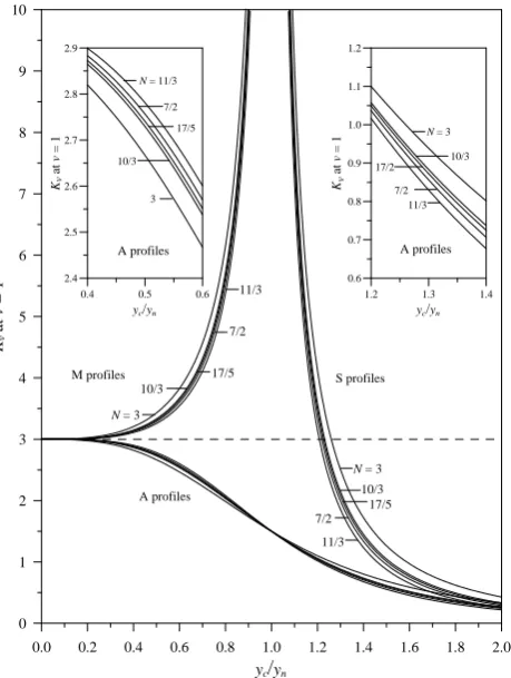
Figure 5. Plot of the curvature, Kv, at v = 1 against yc/yn with the N-value as a

parameter for GVF profiles in sustaining channels and also in adverse channels.

0.0 0.2 0.4 0.6 0.8 1.0 1.2 1.4 1.6 1.8 2.0

yc/yn

0 1 2 3 4 5 6 7 8 9 10

Kv

at

v

= 1

2.4 2.5 2.6 2.7 2.8 2.9

Kv

at

v

= 1

0.4 0.5 0.6 yc/yn

1.2 1.3 1.4 yc/yn 0.6

0.7 0.8 0.9 1.0 1.1 1.2

Kv

at

v

=

1

N = 11/3

7/2 17/5

10/3

11/3

7/2

17/5

N = 3 N = 3

10/3 17/5

11/3 7/2 3

A profiles

A profiles A profiles

S profiles M profiles

N = 3

10/3 17/2

11/3 7/2

Fig. 5. Plot of the curvature,Kv, atv=1 againstyc/ynwith the N

value as a parameter for GVF profiles in sustaining channels and also in adverse channels.

and N value as a parameter, as shown in Fig. 5. The theoret-ical range ofλin this plot is 0≤λ<∞, but it is only plotted for 0≤λ <2 in the figure. An inspection of Fig. 5 reveals thatKvatv=1 for GVF profiles in sustaining channels ap-proaches infinity asλ→1. This trend forKvatv=1 implies that the closer the two v-values at the two inflection points of the M profiles approach unity, as shown in Fig. 3, the larger isKv atv=1, irrespective of the M or S profile, as shown in Fig. 5. In contrast,Kv atv=1 for A profiles in adverse channels decreases and approaches zero asλ → ∞. The A profile corresponding to this limit (λ= ∞)is a vertical line with itsKveverywhere along the line is zero, as manifesting

itself in Fig. 1. As for the effect ofN onKvatv=1, Fig. 5

also shows that the smaller the N value, the larger isKv at v=1 for all M, S, and A profiles in the whole range ofλ, ex-cept that it tends to behave opposite for A profiles spanning 0≤λ≤1.

5.10 Applicability of theyc-based dimensionless GVF profiles

The fact thatyc-based dimensionless GVF profiles obtained

herein by using GHF lies in its capability to reduce the

[image:12.595.315.545.62.367.2] [image:12.595.46.286.533.606.2]

(13)

profiles asyc/yn→0 has laid the foundation to compute at

one sweep theyc-based dimensionless GVF profiles in a

se-ries of sustaining and adverse channels, which have horizon-tal slopes sandwiched in between them. Acceptance of any real numbers by the function parameters (i.e.MandN )of the GHF suggests the practicality of the GHF-based solu-tions to the GVF profiles in channels with cross-sectional shape other than wide rectangle. For applying the GHF-based solutions obtained from Eqs. (3) and (8) to practical prob-lems, our follow-up task needed to be undertaken is the for-mulation of various boundary conditions, which will be in-corporated with the GHF-based solutions to compute at one sweep theyc-based dimensionless GVF profiles in a series

of channels. The accurate formulation of various boundary conditions holds the key of success to compute theyc-based

dimensionless GVF profiles in such a series of channels, though it is perhaps the hardest to develop a reliable method to conduct the computation constrained by such a variety of the boundary conditions.

As for types of the boundary conditions required for com-puting theyc-based dimensionless GVF profiles in a series

of sustaining and adverse channels, we must first locate the internal boundary conditions, which exist at places where the state of flow suddenly changes (Chen and Wang, 1969; Chen and Chow, 1971). One type of the internal boundary conditions needed is at hydraulic jumps and overfalls, which occur in prismatic channels at places where the flow condi-tion changes rapidly from a supercritical state to a subcrit-ical state and vice versa under “freely” flowing conditions. The other type of the internal boundary conditions needed is at sudden or rapid transitions in channel width and cross-sectional shape under “forced” flowing conditions as a re-sult of constricted flows passing through hydraulic structures, such as weirs and sluice gates built in non-prismatic chan-nels. Apparently, there exist various types of the internal boundary conditions, such as the hydraulic-jump equations at places where hydraulic jumps occur, the formation of the critical Froude number at places where overfalls are induced, and the calibrated discharge relations (or rating curves) at places where weirs and sluice gates among other discharge-measuring devices are installed. In fact, it is quite involved to compute theyc-based dimensionless GVF profiles subject to

such a variety of the internal boundary conditions imposed at many places as needed in a series of artificially or natu-rally formed prismatic and non-prismatic channels. It is in-deed challenging to undertake such computation though it is beyond the scope of this paper.

5.11 Comparison of GVF profile obtained by the present method and that by the fourth order Runge–Kutta method

Solving the GVF profile by using a fourth order Runge–Kutta method is in the field of numerical method. The result from the numerical method cannot provide total length of the

wa-ter surface profile with a single computation. The present method can obtain an analytical solution, so it can obtain the water depth at a specified location in a single computa-tion. The computation of Gaussian hypergeometric function is well established in commercial software, such as Matlab and Mathematica. No more programming effort is needed by using the Gaussian hypergeometric function. A comparison of the result obtained by the present method and that by the fourth order Runge–Kutta method is presented in the Supple-ment. For comparison, we take the Example 5.8 in the book of K. Subramanya (2009), with title Flow In Open

Chan-nels. The numerical code written for the commercial

soft-ware Matlab by using the present method, the numerical code for Matlab by using the standard fourth order Runge–Kutta method, and the comparison of M1-profiles obtained by the present method and fourth order Runge–Kutta method are all shown in the Supplement. It is less 10 s for the compu-tations of this example by these two methods. The numeri-cal error in the water depth obtained by the standard fourth order Runge–Kutta method is about 2 % at the longitudinal coordinate x= −8 km.

In addition, it should be noted that the assumption of con-stant hydraulic exponents (MandN) has been made in the direct integration method to solve GVF profiles. Therefore, a suitable choice of representative hydraulic exponents for a concerned channel length is important. Even though, the as-sumption of constant hydraulic exponents is satisfactory in most rectangular and trapezoidal channels, the hydraulic ex-ponents may vary appreciably with respect to the depth of flow when the channel section has abrupt changes in cross-sectional geometry or is topped with a gradually closing crown. In such cases, the channel length should be divided into a number of reaches in each of which the hydraulic exponents appear to be constant (Chow, 1959, p. 260).

6 Conclusions

Success to formulate the normal-depth(yn)-based GVF

pro-files expressed in terms of GHFs for flow in sustaining chan-nels, as reported by Jan and Chen (2012), does not warrant that it can likewise prevail to useynin the normalization of

the GVF equation for flow in horizontal and adverse channels because yn for an assumed uniform flow in horizontal and

adverse channels is undefined. This paper has laid the foun-dation to compute at one sweep the critical-depth(yc)-based

GVF profiles in a series of sustaining and adverse channels, which have horizontal slopes sandwiched in between them. To obtain the GHF-based dimensionless solutions from the

yc-based GVF equation is our first step for developing a

vi-able method to compute the yc-based dimensionless GVF

(14)

we have obtained the GHF-based solutions from theyc-based

dimensionless GVF equation, which proves to be applicable for computing the GVF profiles in both sustaining and ad-verse channels. Secondly, we have analytically proved that the GHF-based dimensionless M and A profiles, if normal-ized byycrather than byyn, can asymptotically reduce to the

yc-based dimensionless H profiles asyc/yn→0. Both

signif-icant results thus constitute the principal conclusions drawn from this study.

In practical applications, theyc-based dimensionless GVF

profiles expressed in terms of the GHF can prove to be more useful, versatile than theyn-based equivalents obtained by

Jan and Chen (2012) though both profiles are convertible to each other through the scaling relations, Eqs. (4) and (5). Among the well-known advantages of suchyc-based

dimen-sionless GVF profiles over their counterparts based on yn,

there lies the most powerful feature of the yc-based GVF

profiles expressed in terms of the GHF, with which one can readily reduce theyc-based M and A profiles asymptotically

to the yc-based H profiles as yc/yn→0. In fact, we have

proved that the M2 and M3 profiles can asymptotically re-duce to the H2 and H3 profiles, respectively, asyc/yn→0;

and so can the A2 and A3 profiles to the H2 and H3 profiles, respectively.

After decades-long struggle by hydraulicians in their at-tempts to improve the rudimentary approach taken to solve the GVF equation using the direct integration method, based onynand the varied-flow function, we have finally come up

with a novel approach to solve the same problem based on

yc and the GHF instead. As shown in Fig. 1, an innovated

formulation of theyc-based dimensionless GVF profiles

ex-pressed in terms of the GHFs has greatly advanced the con-ventional technique used in the GVF computation to the ex-tent that hydraulicians for the first time in the computer age can fully utilize a mathematics software, which is capable of producing the GHF-based solutions of theyc-based

dimen-sionless GVF equation. The principal conclusions so drawn from this study embrace all significant results acquired from the in-depth analysis of theyc-based dimensionless solutions

expressed in terms of the GHF along with those attained in the exact proof of the asymptotic reduction of the yc

-based dimensionless M and A profiles to the corresponding H profiles asyc/yn→0.

Supplementary material related to this article is

available online at: http://www.hydrol-earth-syst-sci.net/ 17/973/2013/hess-17-973-2013-supplement.pdf.

Acknowledgements. Support from the National Science Council

in Taiwan (NSC 100-2221-E-006-202-MY3) to C. D. Jan for this study is acknowledged. The help from W. L. Ke in preparing the supplement is also acknowledged. C. L. Chen was born in 1931 and passed away on 25 January 2012. He was used to be an excellent

hydrologist in US Geological Survey, and a distinguished professor in University of Illinois at Urbana-Champaign and in Utah State University.

Edited by: E. Todini

References

Allen, J. and Enever, K. J.: Water surface profiles in gradually varied open-channel flow, Proceedings, Institute of Civil Engineers, 41, 783–811, 1968.

Bakhmeteff, B. A.: Hydraulics of Open Channels. McGraw-Hill, New York, N.Y., 1932

Chen, C. L.: Unified theory on power laws for flow resistance, J. Hydraul. Eng., ASCE, 117, 371–389, 1991.

Chen, C. L. and Chow, V. T.: Formulation of mathematical watershed-flow model, J. Eng. Mech. Divis., ASCE, 97, 809– 828, 1971.

Chen, C. L. and Wang, C. T.: Nondimensional gradually varied flow profiles, J. Hydraul. Divis., ASCE, 95, 1671–1686, 1969. Chow, V. T.: Integrating the equation of gradually varied flow.

Pro-ceedings Paper No. 838, ASCE, 81, 1–32, 1955.

Chow, V. T.: Closure of Discussions on Integrating the equation of gradually varied flow, J. Hydraul. Divis., ASCE, 83, 9–22, 1957. Chow, V. T.: Open-Channel Hydraulics. McGraw-Hill, New York,

N.Y., 1959.

Jan, C. D. and Chen, C. L.: Use of the Gaussian hypergeometric function to solve the equation of gradually-varied flow, J. Hy-drol., 456–457, 139–145, 2012.

Korn, G. A. and Korn, T. M.: Mathematical Handbook for Scientists and Engineers. McGraw-Hill, New York, N.Y., 1961.

Kumar, A.: Integral solutions of the gradually varied equation for regular and triangular channels. Proceedings, Institute of Civil Engineers, 65, 509–515, 1978.

Kumar, A.: Gradually varied surface profiles in horizontal and ad-versely sloping channels. Proceedings, Institute of Civil Engi-neers, 67, 435–452, 1979.

Kummer, E. E.: ¨Uber die hypergeometrische Reihe, Journal f¨ur die reine und angewandte Mathematik, 15, 39–83 and 127–172, 1836.

Luke, Y. L.: Mathematical Functions and Their Approximations, Academic Press Inc., New York, N.Y., 1975.

Matzke, A. E.: Varied flow in open channels of adverse slope, Trans-actions, ASCE, 102, 651–660, 1937.

Olde Daalhuis, A. B.: Hypergeometric function, in: NIST Hand-book of Mathematical Functions, edited by: Olver, F. W. J., Lozier, D. W., Boisvert, R. F., and Clark, C. W., Cambridge Univ. Press, Cambridge (Chapter 15), 2010.

Pearson, C. E. (Ed.): Handbook of Applied Mathematics, Selected Results and Methods. Van Nostrand Reinhold Company, New York, N.Y., 1974.

Rouse, H.: Critical analysis of open-channel resistance, J. Hydraul. Divis., ASCE, 91, 1–25, 1965.

Seaborn, J. B.: Hypergeometric Functions and Their Applications. Springer-Verlag, New York, N.Y., 1991.

Subramanya, K.: Flow in Open Channels, 3rd Edn. McGraw-Hill, Singapore, 2009.

(15)

455–462, 2012.

Venutelli, M.: Direct integration of the equation of gradually varied flow. J. Irrig. Drain. Eng., ASCE, 130, 88–91, 2004.

Wolfram, S.: The Mathematica Book, third ed. Wolfram Media & Cambridge University Press, Champaign, Illinois, 1996.

Zaghloul, N. A.: A computer model to calculate varied flow func-tions for circular channels, Adv. Eng. Softw., 12, 106–122, 1990. Zaghloul, N. A.: Gradually varied flow in circular channels with