www.hydrol-earth-syst-sci.net/20/3289/2016/ doi:10.5194/hess-20-3289-2016
© Author(s) 2016. CC Attribution 3.0 License.
A Bayesian consistent dual ensemble Kalman filter for
state-parameter estimation in subsurface hydrology
Boujemaa Ait-El-Fquih1, Mohamad El Gharamti1,2, and Ibrahim Hoteit1
1Department of Earth Sciences and Engineering, King Abdullah University of Science and Technology (KAUST),
23955-6900 Thuwal, Kingdom of Saudi Arabia
2Mohn-Sverdrup Center for Global Ocean Studies and Operational Oceanography, Nansen Environmental and Remote
Sensing Center (NERSC), 5006 Bergen, Norway
Correspondence to:Ibrahim Hoteit ([email protected])
Received: 16 December 2015 – Published in Hydrol. Earth Syst. Sci. Discuss.: 1 February 2016 Revised: 29 June 2016 – Accepted: 10 July 2016 – Published: 12 August 2016
Abstract.Ensemble Kalman filtering (EnKF) is an efficient approach to addressing uncertainties in subsurface ground-water models. The EnKF sequentially integrates field data into simulation models to obtain a better characterization of the model’s state and parameters. These are generally esti-mated following joint and dual filtering strategies, in which, at each assimilation cycle, a forecast step by the model is followed by an update step with incoming observations. The joint EnKF directly updates the augmented state-parameter vector, whereas the dual EnKF empirically employs two sep-arate filters, first estimating the parameters and then estimat-ing the state based on the updated parameters. To develop a Bayesian consistent dual approach and improve the state-parameter estimates and their consistency, we propose in this paper a one-step-ahead (OSA) smoothing formulation of the state-parameter Bayesian filtering problem from which we derive a new dual-type EnKF, the dual EnKFOSA. Compared
with the standard dual EnKF, it imposes a new update step to the state, which is shown to enhance the performance of the dual approach with almost no increase in the computa-tional cost. Numerical experiments are conducted with a two-dimensional (2-D) synthetic groundwater aquifer model to investigate the performance and robustness of the proposed dual EnKFOSA, and to evaluate its results against those of
the joint and dual EnKFs. The proposed scheme is able to successfully recover both the hydraulic head and the aquifer conductivity, providing further reliable estimates of their un-certainties. Furthermore, it is found to be more robust to dif-ferent assimilation settings, such as the spatial and temporal distribution of the observations, and the level of noise in the
data. Based on our experimental setups, it yields up to 25 % more accurate state and parameter estimations than the joint and dual approaches.
1 Introduction
procedure of pinpointing parameter values that, when in-tegrated with the simulation models, allow some system-response variables (e.g., hydraulic head, solute concentra-tion) to fit given observations (Vrugt et al., 2003; Valstar et al., 2004; Alcolea et al., 2006; Feyen et al., 2007; Hen-dricks Franssen and Kinzelbach, 2009; Zhou et al., 2014). Recently, sequential data assimilation techniques, such as the particle filter (PF), have been proposed to handle any type of statistical distribution, Gaussian or not, to properly deal with strongly nonlinear systems (Chang et al., 2012). The PF may require, however, a prohibitive number of particles (and thus model runs) to accurately sample the distribution of the state and parameters, making this scheme computationally inten-sive for large-scale hydrological applications (Doucet et al., 2001; Moradkhani et al., 2005a; Hoteit et al., 2008; Montzka et al., 2011). This problem has been partially addressed by the popular ensemble Kalman filter (EnKF), which further provides robustness, efficiency, and non-intrusive formula-tion (Reichle et al., 2002; Vrugt et al., 2006; Zhou et al., 2011; Gharamti et al., 2013; Panzeri et al., 2014; Crestani et al., 2013; McMillam et al., 2013; Erdal and Cirpka, 2016) to tackle the state-parameter estimation problem.
The EnKF is a filtering technique that is relatively simple to implement, even with complex nonlinear models, requir-ing only an observation operator that maps the state variables from the model space into the observation space. Compared with traditional inverse and direct optimization techniques, which are generally based on least-squares-like formulations, the EnKF has the advantage of being able to account for model errors that are present not only in the uncertain param-eters but also in the external forcings (Hendricks Franssen and Kinzelbach, 2008). Because of its sequential formula-tion, the EnKF does not require one to store all past informa-tion about the states and parameters, leading to consequent savings in computational cost (McLaughlin, 2002; Gharamti et al., 2014b).
The EnKF is widely used in surface and subsurface hydro-logical studies to tackle state-parameter estimation problems (Zhou et al., 2014; Panzeri et al., 2014). Two approaches are usually considered based on the joint and the dual estima-tion strategies. The standard joint approach concurrently es-timates the state and the parameters by augmenting (in the same vector) the state variables with the unknown parame-ters, that do not vary in time. The parameters could also be set to follow an artificial evolution (random walk) before they get updated with incoming observations (Wan et al., 1999). One of the early applications of the joint EnKF to subsurface groundwater flow models was presented by Chen and Zhang (2006). In their study, a conceptual subsurface flow system was considered and ensemble filtering was performed to es-timate the transient pressure field alongside the hydraulic conductivity. In a reservoir engineering application, Næv-dal et al. (2005) considered a two-dimensional (2-D) North Sea field model and considered the joint estimation prob-lem of the dynamic pressure and saturation on top of the
static permeability field. Groundwater contamination prob-lems were also tackled using the joint EnKF (e.g., Li et al., 2012; Gharamti and Hoteit, 2014), in which the hydraulic head, contaminant concentration, and spatially variable per-meability and porosity parameters were estimated for cou-pled groundwater flow and contaminant transport systems.
Several studies argued that the joint EnKF may suffer from important inconsistencies between the estimated state and parameters that could degrade the filter performance, espe-cially with large-dimensional and strongly nonlinear systems (e.g., Moradkhani et al., 2005b; Chen and Zhang, 2006; Wen and Chen, 2007). One classical approach that has been pro-posed to tackle this issue is the so-called dual filter, which separately updates the state and parameters using two in-teractive EnKFs, one acting on the state and the other on the parameters (Moradkhani et al., 2005b). The dual EnKF has been applied to streamflow forecasting problems using rainfall–runoff models (e.g., Lü et al., 2013; Samuel et al., 2014), subsurface contaminant (e.g., Tian et al., 2008; Lü et al., 2011; Gharamti et al., 2014b), and compositional flow models (e.g., Phale and Oliver, 2011; Gharamti et al., 2014a), to cite but a few. Gharamti et al. (2014a) concluded that the dual scheme provides more accurate state and param-eter estimations than the joint scheme when implemented with large enough ensembles. In terms of complexity, how-ever, the dual scheme requires integrating the filter ensem-ble twice with the numerical model at every assimilation cy-cle, and is therefore computationally more demanding. In re-lated works, Gharamti et al. (2013) extended the dual filter-ing scheme to tackle the state estimation problem of one-way coupled models, and to the framework of hybrid-EnKF (Gharamti et al., 2014b).
The dual filter has been basically introduced as a heuris-tic scheme and is not consistent with the Bayesian filtering framework (Hendricks Franssen and Kinzelbach, 2008). A first attempt to build a Bayesian consistent dual-like filter was recently proposed by Gharamti et al. (2015) in which a new joint EnKF scheme was derived following the one-step-ahead (OSA) smoothing formulation of the Bayesian filter-ing problem. The new joint scheme reverses the order of the measurement-update and the forecast (or time) update, lead-ing to two Kalman-like update steps based on the current ob-servations: one for state smoothing and one for parameters updating.
Motivated by the promising results of Gharamti et al. (2015), we follow here the same OSA smoothing formula-tion to derive a new dual EnKF, which we refer to as the dual EnKFOSA hereafter, generalizing the joint scheme of
im-posed by Gharamti et al. (2015). Exploiting the conditional dependency between the state and its observation leads to one more Kalman-like update of the state, generalizing the joint scheme of Gharamti et al. (2015), at practically no in-crease in the computational cost. Likewise, the new dual fil-tering scheme is not only more general than the standard dual scheme, but also explicitly derives the conditions un-der which the (heuristic) steps of the standard dual EnKF can be derived within a Bayesian framework. Synthetic nu-merical experiments based on a groundwater flow model and estimating the hydraulic head and the conductivity parame-ter field, are conducted to assess the performance of the pro-posed dual EnKFOSAand to compare its results against those
of the joint and the dual EnKFs, which we consider as ref-erences to evaluate the behavior of the dual EnKFOSA. The
numerical results suggest that the proposed scheme is ben-eficial in terms of estimation accuracy compared to the two standard joint and dual schemes, and is more robust to vari-ous experimental settings and observational scenarios.
The rest of the paper is organized as follows. Section 2 re-views the standard joint and dual EnKF strategies. The dual EnKFOSAis derived in Sect. 3 and its relation with the joint
and dual EnKFs is discussed. Section 4 presents a concep-tual groundwater flow model and outlines the experimen-tal setup. Numerical results are presented and discussed in Sect. 5. Conclusions are offered in Sect. 6, followed by an Appendix.
2 Joint and dual ensemble Kalman filtering 2.1 Problem formulation
Consider a discrete-time state-parameter dynamical system:
xn=Mn−1(xn−1, θ )+ηn−1
yn=Hnxn+εn , (1)
wherexn∈RNx andyn∈RNy denote the system state and the observation at timetnof dimensionsNxandNy, respectively,
andθ∈RNθ is the parameter vector of dimensionN
θ.Mnis
a nonlinear operator integrating the system state from time
tn totn+1, and the observational operator at timetn,Hn, is
assumed to be linear for simplicity; the proposed scheme can be easily extended to the nonlinear case1. The model pro-cess noise, η= {ηn}n∈N, and the observation process noise, ε= {εn}n∈N, are assumed to be independent, jointly
indepen-dent, and independent ofx0andθ. Furthermore, letηnandεn
be Gaussian with zero means and covariancesQnandRn,
re-spectively. Throughout the paper,y0:n def
= {y0,y1,· · ·,yn}and
p(xn)andp(xn|y0:l)stand for the prior probability density
function (pdf) ofxnand the posterior pdf ofxngiveny0:l,
re-spectively. All other pdf’s used are defined in a similar way.
1The termH
nxf,(m)n is replaced byHn(xf,(m)n )in Eq. (26), and
Hnξn(m)is replaced byHn(ξn(m))in Eq. (34).
We focus on the state-parameter filtering problem, i.e., the estimation at each time, tn, of the state, xn, as well as the
parameters vector, θ, from the history of the observations, y0:n. The standard solution of this problem is the a posteriori
mean (AM):
Ep(xn|y0:n)[xn]=
Z
xnp (xn, θ|y0:n)dxndθ, (2)
Ep(θ|y0:n)[θ] =
Z
θp (xn, θ|y0:n)dxndθ, (3)
which minimizes the a posteriori mean square error. In prac-tice, analytical computation of Eqs. (2) and (3) is not feasible, mainly due to the nonlinear character of the system. The joint and dual EnKFs have been introduced as efficient schemes to compute approximations of Eqs. (2) and (3). These algo-rithms are reviewed in the next section.
2.2 The joint and dual EnKFs 2.2.1 The joint EnKF
The key idea behind the joint EnKF is to transform the state-parameter system (Eq. 1) into a classical state-space system based on the augmented state,zn=xTnθT
T
, on which the classical EnKF can be directly applied. The new augmented state-space system can be written as
zn=Mfn−1(zn−1)+eηn−1
yn=eHnzn+εn
, (4)
whereMfn−1(zn−1)=
Mn−1(zn−1)
θ
,eηn−1= [ηTn−1 0]T, e
Hn= [Hn0], with 0 a zero matrix with appropriate
di-mensions. xf,(m)n ,xa,(m)n , and xs,(m)n respectively denote the
mth forecast, analysis, and (OSA) smoothing member of the state,xn, whileθ|(m)n denotes themth sample of the
parame-ters posterior pdf,p(θ|y0:n). Since the parameters are static
(i.e., time-independent),θ|(m)n ,n=1, 2,· · ·, could be consid-ered as analysis, forecast, or smoothing members.
Starting at timetn−1from an analysis ensemble of sizeNe,
{xa,(m)n−1 ,θ|(m)n−1}Ne
m=1sampled fromp(zn−1|y0:n−1), the EnKF
uses the augmented state model (1st equation of Eq. 4) to compute the forecast ensemble,{xf,(m)n ,θ|(m)n−1}
Ne
m=1,
approx-imatingp(zn|y0:n−1). The observation model (2nd equation
of Eq. 4) is then used to obtain the analysis ensemble,{xa,(m)n ,
θ|(m)n }Ne
m=1, at timetn. Let, for an ensemble{r(m)}Nme=1,ˆr
de-note its empirical mean and Sr a matrix withNe-columns
whosemth column is defined as(r(m)− ˆr). The joint EnKF steps can be summarized as follows:
xf,(m)n =Mn−1
xa,(m)n−1, θ|(m)n−1+η(m)n−1; η(m)n−1
∼N(0,Qn−1) . (5)
The state forecast estimate, which is the mean of
p(xn|y0:n−1) (i.e., Ep(xn|y0:n−1)[xn]), is taken as the
empirical mean of the forecast ensemble, xˆfn. The associated forecast error covariance is estimated as Pxf
n=(Ne−1)
−1S xf
nS
T xf
n.
– Analysis step: once a new observation is available, all members,xf,(m)n andθ|(m)n−1, are updated as in the Kalman
filter (KF):
yf,(m)n =Hnxf,(m)n +ε(m)n ; ε(m)n ∼N(0,Rn) , (6)
xa,(m)n =xf,(m)n +Pxf n,yfnP
−1 yf
n
yn−yf,(m)n
| {z }
µ(m)n
, (7)
θ|(m)n =θ|(m)n−1+Pθ
|n−1,ynf·µ
(m)
n . (8)
The (cross-)covariances in Eqs. (7) and (8) are practi-cally evaluated from the ensembles as
Pxf
n,ynf =(Ne−1) −1S
xf nS
T yf
n, (9)
Pyf
n=(Ne−1)
−1S yf
nS
T yf
n, (10)
Pθ
|n−1,yfn=(Ne−1)
−1S θ|n−1S
T yf
n. (11)
The analysis estimates, Eqs. (2) and (3), and their error covariances, can thus be approxi-mated by the analysis ensemble means, xˆan and
ˆ
θ|n, and covariances Pxa
n=(Ne−1)
−1S xa
nS
T xa
n and
Pθ|n=(Ne−1) −1S
θ|nS
T
θ|n, respectively. Note that
Pxf n,ynfP
−1 yf
n in Eq. (7) represents the Kalman Gain,
Pxf
nH
T n[HnPxf
nH
T
n +Rn]−1. This statistical
formula-tion of the Kalman gain offers more flexibility to deal with nonlinear observational operators (Moradkhani et al., 2005b).
2.2.2 The dual EnKF
In contrast with the joint EnKF, the dual EnKF is empirically designed following a conditional estimation strategy, oper-ating as a succession of two EnKF-like filters. First, a (pa-rameter) filter is applied to compute{θ|(m)n }Ne
m=1from{x a,(m) n−1 ,
θ|(m)n−1}Ne
m=1exactly as in the joint EnKF:
– Forecast step: the parameters ensemble,{θ|(m)n−1}Ne
m=1, is
kept invariant, while the state samples are integrated in time as in Eq. (5) to compute the forecast ensemble, {xf,(m)n }Nme=1.
– Analysis step: as in Eq. (6), the observation forecast ensemble {yf,(m)n }Nme=1 is computed from {x
f,(m) n }Nme=1.
This is then used to update the parameters ensemble, {θ|(m)n }Ne
m=1, following Eq. (8).
Another (state) filter is then applied to compute{xa,(m)n }Nme=1
from {xa,(m)n−1 }Ne
m=1 as well as the new parameter ensemble,
{θ|(m)n }Ne
m=1, again in two steps that can be summarized as
fol-lows.
– Forecast step: each member, xa,(m)n−1 , is propagated in time with the dynamical model using the updated pa-rameters ensemble:
ex f,(m)
n =Mn−1
xa,(m)n−1 , θ|(m)n . (12)
– Analysis step: as in the parameter filter,{
ey f,(m) n }Nme=1is
computed from{
ex f,(m)
n }Nme=1using Eq. (6), which finally
yields{xa,(m)n }Nme=1as in Eq. (7).
To better understand how the dual EnKF differs from the joint EnKF, we focus on how the analysis members at time
tn, namely,xa,(m)n andθ|(m)n , are obtained starting from their
counterparts at previous time,xa,(m)n−1 andθ|(m)
n−1. The
parame-ters members,θ|(m)n , are computed based on the same equa-tion (Eq. 8) in both algorithms. For the state members,xa,(m)n ,
we have
xa,(m)n joint EnKF= Mn−1
xa,(m)n−1 , θ|(m)n−1+Pxf n,ynf
P−1
yf n
yn−yf,(m)n
| {z }
µ(m)n
, (13)
xa,(m)n dual EnKF= Mn−1
xa,(m)n−1 ,
θ|n(m)
z }| {
θ|(m)n−1+Pθ
|n−1,yfn·µ
(m) n
| {z }
ex f,(m) n +P ex f n,ey
f nP −1 ey f n
yn−ey f,(m) n
| {z }
e
µ(m)n
. (14)
For simplicity, we ignore here the process noise term, ηn,
which is commonly applied in geophysical applications. As one can see, the joint EnKF updates the state members us-ing one Kalman-like correction (term ofµ(m)n in Eq. (13)),
the “forecast” membersexf,(m)n . Theex f,(m)
n are finally updated
using a Kalman-like correction (term ofeµ(m)n in Eq. 14), to
obtain the analysis membersxa,(m)n . Such a separation of the update steps is expected to provide more consistent estimates of the parameters. The dual update framework was indeed shown to provide better performances than the joint EnKF, at the cost of increased computational burden (see for instance, Moradkhani et al., 2005b; Samuel et al., 2014; Gharamti et al., 2014a).
2.2.3 Probabilistic formulation
Following a probabilistic formulation, the augmented state system (Eq. 4) can be viewed as a continuous state hidden Markov chain with transition density,
p (zn|zn−1)=p (xn|xn−1, θ ) p(θ|θ )
=Nxn(Mn−1(xn−1, θ ) ,Qn−1) , (15)
and likelihood,
p (yn|zn)=p (yn|xn)=Nyn(Hnxn,Rn) , (16)
where Nv(m,C)represents a Gaussian pdf of argumentv
and parameters (m,C).
One can then easily verify that the joint EnKF can be de-rived from a direct application of two classical results of ran-dom sampling (Properties 1 and 2 in Appendix A) on the following classical generic formulas:
p (zn|y0:n−1)=
Z
p (xn|xn−1, θ ) p (zn−1|y0:n−1)dxn−1, (17) p (yn|y0:n−1)=
Z
p (yn|xn) p (xn|y0:n−1)dxn, (18)
p (zn|y0:n)=
p (zn,yn|y0:n−1)
p (yn|y0:n−1)
. (19)
Equation (17) refers to a Markovian step (or time-update step) and uses the transition pdf, p(xn|xn−1, θ ), of the
Markov chain,{zn}n, to compute the forecast pdf ofznfrom
the previous analysis pdf. Equation (19) refers to a Bayesian step (or measurement-update step) since it uses the Bayes’ rule to update the forecast pdf of zn using the current
ob-servation yn. Thus, establishing the link between the joint
EnKF and Eqs. (17)–(19), one can show that Property 1 and Eq. (17) lead to the forecast ensemble of the state (Eq. 5). Property 1 and Eq. (18) lead to the forecast ensemble of the observations (Eq. 6). Property 2 and Eq. (19) then provide the analysis ensemble of the state (Eq. 7) and the parameters (Eq. 8).
Regarding the dual EnKF, the forecast ensemble of the state and observations in the parameter filter can be obtained following the same process as in the joint EnKF. This is fol-lowed by the computation of the analysis ensemble of the parameters using Property 2 and
p (θ|y0:n)=
p (θ,yn|y0:n−1)
p (yn|y0:n−1)
. (20)
However, in the state filter, the ensemble,{
ex f,(m)
n }Nme=1,
ob-tained via Eq. (12) in the forecast step does not represent the forecast pdf,p(xn|y0:n−1), since Eq. (12) involvesθ|(m)n
rather thanθ|(m)n−1. Accordingly, the dual EnKF is basically a heuristic algorithm in spite of its proven performance.
3 One-step-ahead smoothing-based dual EnKF (dual EnKFOSA)
The classical (time-update, measurement-update) path (Eqs. 17–19) to compute the analysis pdfp(zn|y0:n)from
p(zn−1|y0:n−1) is not the only possible one. One may
in-deed reverse the order of the time- and measurement-update steps by involving the OSA smoothing pdf, p(zn−1|y0:n),
between two successive analysis pdf’s:p(zn−1|y0:n−1)and
p(zn|y0:n). Desbouvries et al. (2011) considered the OSA
smoothing-based filtering problem in low-dimensional state-space systems to derive a class of KF- and PF-like algo-rithms for filtering the state. The more recent work of Lee and Farmer (2014) proposed a number of algorithms to es-timate both the system state and the model noise based on a similar strategy. In the context of large-dimensional state-parameters filtering, we show in this section that this leads to a new fully Bayesian consistent dual-like filtering scheme, the dual EnKFOSA, which, compared to the standard dual
EnKF, not only introduces another Kalman-like update of the state but also involves a (new) smoothing step that constraints the state with the future observation. Exploiting the future observation should be particularly beneficial in the context of the EnKF as it includes more information in the estimation process that may help mitigating for the suboptimal character of the EnKF-like methods, being formulated under a linear Gaussian framework, and usually implemented with limited ensembles and crude approximate noise statistics.
3.1 The one-step-ahead smoothing-based dual filtering algorithm
The analysis pdf, p(xn, θ|y0:n), can be computed from
p(xn−1,θ|y0:n−1)in two steps:
– Smoothing step: the one-step-ahead smoothing pdf,
p(xn−1,θ|y0:n), is first computed as
p (xn−1, θ|y0:n)∝p (yn|xn−1, θ,y0:n−1)
p (xn−1, θ|y0:n−1) , (21)
with,
p (yn|xn−1, θ,y0:n−1)= Z
p (yn|xn,xn−1, θ,y0:n−1)
p (xn|xn−1, θ,y0:n−1)dxn,= Z
p (yn|xn)
Equation (22) is derived from the fact that in the state-parameter model (Eq. 1), the observation noise,εn, and
the model noise,ηn−1, are independent of(xn−1,θ )and
past observationsy0:n−1.
The smoothing step (Eq. 21) is indeed a measurement-update step since, giveny0:n−1, Eq. (21) translates the
computation of the posterior,p(xn−1,θ|yn), as a
nor-malized product of the prior,p(xn−1,θ ), and the
likeli-hood,p(yn|xn−1,θ )(note from Eq. (22) thatp(yn|xn−1,
θ,y0:n−1)=p(yn|xn−1,θ )).
– Forecast step: the smoothing pdf attn−1is then used to
compute the current analysis pdf,p(xn,θ|y0:n), as
p(xn, θ|y0:n)= Z
p (xn|xn−1, θ,y0:n)
p (xn−1, θ|y0:n)dxn−1, (23)
with,
p (xn|xn−1, θ,y0:n)∝p (yn|xn) p (xn|xn−1, θ ) , (24)
which, in turn, arises from the fact thatεnandηn−1are
independent of (xn−1,θ) andy0:n−1(see smoothing step
above). We note here that only the (marginal) analysis pdf ofxn,p(xn|y0:n), is of interest since the analysis pdf
ofθhas already been computed in the smoothing step. From Eq. (24),p(xn|xn−1,θ,y0:n)=p(xn|xn−1,θ,yn).
Thereby, there is a similarity between Eq. (23) and the forecast step (Eq. 17) in the sense that Eq. (23) can be seen as a forecast step once the observationynis known;
i.e., Eq. (23) coincides with “Eq. (17) given the obser-vationyn”. Accordingly, and without abuse of language,
we refer to Eqs. (23)–(24) as the forecast step. 3.2 Ensemble formulation
Since it is not possible to derive the analytical solution of Eqs. (21)–(24) because of the nonlinear character of the model, M(.), we use Properties 1 and 2 (see Appendix A) to propose an EnKF-like formulation, assuming that p(yn,
zn−1|y0:n−1) is Gaussian for all n. This assumption
im-plies thatp(zn−1|y0:n−1),p(zn−1|y0:n), andp(yn|y0:n−1)are
Gaussian.
3.2.1 Smoothing step
Starting at time tn−1, from an analysis ensemble, {xa,(m)n−1 ,
θ|(m) n−1}
Ne
m=1, one can use Property 1 in Eq. (22) to sample the
observation forecast ensemble,{yf,(m)n }Nme=1, as
xf,(m)n =Mn−1
xa,(m)n−1, θ|(m)n−1+η(m)n−1, (25) yf,(m)n =Hnxf,(m)n +ε(m)n , (26)
withηn(m)−1∼N(0,Qn−1)andεn(m)∼N(0,Rn). Property 2 is
then used in Eq. (21) to compute the smoothing ensemble,
{xs,(m)n−1,θ|(m)
n }
Ne
m=1, as
xs,(m)n−1 =xa,(m)n−1 +Pxa n−1,ynfP
−1 yf
n
yn−yf,(m)n
| {z }
νn(m)
, (27)
θ|(m)n =θ|(m)n−1+Pθ
|n−1,ynf·ν
(m)
n . (28)
The (cross-) covariances in Eqs. (27) and (28) are defined and evaluated similarly to Eqs. (9)–(11).
3.2.2 Forecast step
The analysis ensemble, {xa,(m)n }Nme=1, can be obtained from
{xs,(m)n−1,θ|(m)
n }
Ne
m=1 using Property 1 in Eq. (23), once the a
posteriori transition pdf,p(xn|xn−1,θ,yn), is computed via
Eq. (24). Furthermore, one can verify that Eq. (24) leads to a Gaussian pdf:
p (xn|xn−1, θ,yn)=Nxn(Mn−1(xn−1, θ )
+Ken(yn−HnMn−1(xn−1, θ )) ,eQn−1, (29)
with eKn=Qn−1HTn[HnQn−1HTn +Rn]−1 and e
Qn−1=Qn−1−eKnHnQn−1. However, when the state
dimension,Nx, is very large, the computational cost ofeKn
andeQn−1(which may be a non-diagonal matrix even when
Qn−1 is diagonal) may become prohibitive. One way to
avoid this problem is to directly sample fromp(xn|xn−1,θ,
yn) without explicitly computing this pdf in Eq. (29). Let
{
ex (m)
n (xn−1,θ )}Nme=1denotes an ensemble of samples drawn
from p(xn|xn−1, θ, yn). The notationex (m)
n (xn−1, θ )refers
to a functionex(m)n of (xn−1,θ ); similar notations hold for eξ
(m)
n (.)andey (m)
n (.)in Eqs. (30) and (31), respectively. Using
Properties 1 and 2, an explicit form of such samples can be obtained as (see Appendix B)
eξn(m)(xn−1, θ )=Mn−1(xn−1, θ )+η(m)n−1; η (m) n−1
∼N(0,Qn−1) , (30)
ey (m)
n (xn−1, θ )=Hneξn(m)(xn−1, θ )+εn(m); εn(m)
∼N(0,Rn) , (31)
ex (m)
n (xn−1, θ )=eξn(m)(xn−1, θ )+Peξn,eyn
P−1
e
yn
h
yn−ey (m)
n (xn−1, θ ) i
, (32)
where the (cross)-covariances,P
eξn,eyn
andP
eyn, are evaluated
from the ensembles {eξ (m)
n (xn−1, θ )}mNe=1 and {yen (m)(x
n−1,
θ )}Ne
m=1, similarly to Eqs. (9)–(11). Now, using Property 1 in
Eq. (23), one can compute an analysis ensemble,{xa,(m)n }Nme=1,
from the smoothing ensemble, {xs,(m)n−1, θ|(m)
n }
Ne
m=1, using
the functional form Eq. (32). More precisely, we ob-tain, xa,(m)n =ex
(m)
n (xs,(m)n−1, θ (m)
|n ), which is equivalent to set
xn−1=xs,(m)n−1 andθ=θ (m)
3.2.3 Summary of the dual EnKFOSAalgorithm
Starting from an analysis ensemble, {xa,(m)n−1 , θ|(m)n−1}Ne
m=1, at
timetn−1, the updated ensemble of both state and
parame-ters at timetnis obtained with the following two steps:
– Smoothing step: the state forecast ensemble, {xf,(m)n }Ne
m=1, is first computed by Eq. (25), and then
used to compute the observation forecast ensemble, {yf,(m)n }Nme=1, as in Eq. (26). The observation forecast
ensemble is then used to compute the one-step-ahead smoothing ensemble of the state, {xs,(m)n−1 }Ne
m=1, and
parameters, {θ|(m)
n }
Ne
m=1, based on the Kalman-like
updates (Eqs. 27 and 28), respectively.
– Forecast step: the analysis ensemble of the state {xa,(m)n }Nme=1is obtained as
ξn(m)=Mn−1
xs,(m)n−1, θ|(m)n +η(m)n−1;η(m)n−1
∼N(0,Qn−1) , (33)
ey f,(m)
n =Hnξn(m)+ε(m)n ; ε(m)n ∼N(0,Rn) , (34)
xa,(m)n =ξn(m)+Pξ
n,ey f nP
−1
e
yf n
yn−ey f,(m) n
, (35)
with Pξ
n,ey f
n=(Ne−1)
−1S ξnS
T
ey f n
and P
ey f
n=(Ne−1)
−1
S
eynfS
T
ey f n
.
The proposed dual EnKFOSAis an ensemble
implementa-tion, under the common Gaussian assumpimplementa-tion, of the generic Bayesian filtering algorithm presented in Sect. 3.1. This jus-tifies its Bayesian consistency in contrast with the stan-dard dual EnKF, which, as discussed in Sect. 2.2.3, lacks a Bayesian interpretation. In contrast with the dual EnKF, which uses θ|(m)n andxa,(m)n−1 to computexa,(m)n (see Eq. 14),
the proposed dual EnKFOSAusesθ|(m)n and the smoothed state
members,xs,(m)n−1, which are thexa,(m)n−1 after an update with the current observation,yn, following Eq. (27). Therefore, when
including the Kalman-like correction term as well, the obser-vation, yn, is used 3 times in the dual EnKFOSA in a fully
consistent Bayesian formulation, compared to only twice in the dual EnKF. This means that the dual EnKFOSAexploits
the observations more efficiently than the dual EnKF, which should provide more information for improved and more consistent state and parameters estimates. Note that the dual EnKFOSAreduces to the dual EnKF in the particular case of
a perfect model andxs,(m)n−1 =xa,(m)n−1 .
The joint EnKFOSA of Gharamti et al. (2015) has been
derived following the same approach under the assump-tion of independence between the state, xn, and its
obser-vation, yn, given the previous state, xn−1, and parameters,
θ (assumption (16) in Gharamti et al., 2015). This assump-tion has been adopted to avoid evaluating the computaassump-tion- computation-ally demanding term p(xn|xn−1,θ,yn)by replacing it with
the more easily sampled state transition pdf, p(xn|xn−1,
θ )=Nxn(Mn−1(xn−1,θ ),Qn−1), to draw the state
analy-sis ensemble. Here, we propose a more efficient approach to directly sample the analysis ensemble without explicitly computingp(xn|xn−1, θ,yn)and without the need of any
additional assumption. The joint EnKFOSAis therefore a
par-ticular case of the dual EnKFOSA, involving two Kalman-like
updates only (those of the smoothing step), since in the fore-cast step, the state analysis members,xa,(m)n , are computed
from the smoothed members,(xs,(m)n−1, θ|(m)n ), by integrating them with the model and without any update with the current observation. More specifically, Eqs. (33)–(35) above reduce in Gharamti et al. (2015) to Eq. (33) (i.e.,xa,(m)n =ξn(m)).
Despite the smoothing formulation of the dual EnKFOSA,
this algorithm obviously addresses the state forecast problem as well. As discussed in the smoothing step above, the (one-step-ahead) forecast members are inherently computed. The
j-step-ahead forecast member, denoted byx(m)n+j|n forj≥2, can be computed following a recursive procedure where, for
`=2, 3,· · ·,j, one has
x(m)n+`|n=Mn+`−1
x(m)n+`−1|n, θ|(m)n +ηn(m)+`−1, η(m)n+`−1
∼N(0,Qn+`−1) . (36)
3.3 Complexity of the joint EnKF, dual EnKF, and dual EnKFOSA
The computational complexity of the different state-parameter EnKF schemes can be split between the forecast (time-update) step and the analysis (measurement-update) step. The joint EnKF requiresNemodel runs (for forecasting
the state ensemble) andNeKalman corrections (for updating
the forecast ensemble). This is practically doubled when us-ing the dual EnKF, since the latter requires 2Ne model runs
and 2NeKalman corrections:Necorrections for each of the
forecast state ensemble and the forecast parameter ensem-ble. As presented in the previous section, the dual EnKFOSA
smoothes the state estimate at the previous time step before updating the parameters and the state at the current time. Thus, the dual EnKFOSArequires as many model runs (2Ne)
as the dual EnKF, and an additionalNe correction steps to
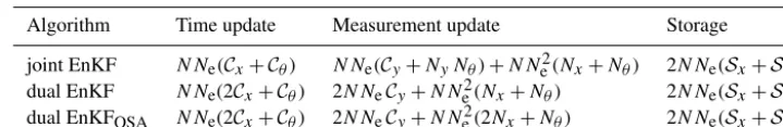
apply smoothing. In large-scale geophysical applications, the correction step of the ensemble members is often computa-tionally not significant compared to the cost of integrating the model in the forecast step. The approximate computa-tional complexity and memory storage for each algorithm are summarized in Table 1. The tabulated complexities for each method are valid under the assumption thatNyNx; i.e.,
Table 1.Approximate computational complexities of the joint EnKF, the dual EnKF, and the dual EnKFOSAalgorithms. Notations are as follows.Nx: number of state variables,Nθ: number of parameter variables,Ny: number of observations,N: number of assimilation cycles, Ne: ensemble size,Cx: state model cost (i.e.,Nx2 is the linear KF),Cθ: parameter model cost (usually free≡identity),Cy: observation
operator cost (i.e.,NyNxin the linear KF),Sx: storage volume for one state vector, andSθ: storage volume for one parameter vector.
Algorithm Time update Measurement update Storage joint EnKF N Ne(Cx+Cθ) N Ne(Cy+NyNθ)+N Ne2(Nx+Nθ) 2N Ne(Sx+Sθ)
dual EnKF N Ne(2Cx+Cθ) 2N NeCy+N Ne2(Nx+Nθ) 2N Ne(Sx+Sθ)
dual EnKFOSA N Ne(2Cx+Cθ) 2N NeCy+N Ne2(2Nx+Nθ) 2N Ne(Sx+Sθ)
4 Numerical experiments
4.1 Transient groundwater flow problem
We adopt in this study the subsurface flow problem of Bai-ley and Baú (2010). The system consists of a 2-D transient flow with an areal aquifer area of 0.5 km2 (Fig. 1). Con-stant head boundaries of 20 and 15 m are placed on the west and east ends of the aquifer, respectively, with an average saturated thickness,b, of 25 m. The height of the imperme-able aquifer bottom,zbot, is assumed constant (i.e., horizontal
aquifer bottom). The north and south boundaries are assumed to be impermeable (Fig. 1). The mesh is discretized using a cell-centered finite difference scheme with 10 m×20 m rect-angles, resulting in 2500 elements. The following 2-D satu-rated groundwater flow system is solved:
∂ ∂x
Tx
∂h ∂x
+ ∂
∂y
Ty
∂h ∂y
=S∂h
∂t +q, (37)
whereT is the transmissivity [L2T−1], which is related to
the conductivity, K, through T=K b, h is the hydraulic head [L], t is time [T], S is storativity [–], and q de-notes the sources as recharge or sinks due to pumping wells [L T−1]. Unconfined aquifer conditions are simulated by setting S=0.20 to represent the specific yield. A log-conductivity field is generated using the sequential Gaus-sian simulation toolbox, GCOSIM3D (Gómez-Hernández and Journel, 1993), with a geometric mean of 10−13m s−1, a variance of Y=logK equal to 1.5, and a Gaussian var-iogram with a range equal to 250 m in the x direction and 500 m in theydirection (Fig. 1).
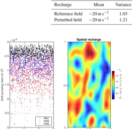
We consider a dynamically complex experimental set-ting involving various time-dependent external forcings. The recharge is assumed spatially heterogenous and sampled us-ing the GCOSIM3D toolbox (Gómez-Hernández and Jour-nel, 1993) with statistical parameters shown in Table 2. Three different pumping wells (PW) are inserted within the aquifer domain and can be seen in Fig. 1 (square symbols). From these wells, transient pumping of groundwater takes place with different daily values as plotted in the left panel of Fig. 2. The highest pumping rates are associated with PW2 with an average daily rate of 0.0513 m day−1. Smaller
0 0.25 0.5
0 0.5 1
-16 -15.5 -15 -14.5 -14 -13.5 -13 -12.5 -12 -11.5
No flow
No flow
Co
ns
ta
nt
hy
dr
au
lic
he
ad,
h
=
15
m
(st
re
am
)
Distance (km)
C
on
st
ant
hy
dr
aul
ic
he
ad,
h
=
20
m
Y= log K, for K in m s
PW2 MW1
PW1
CW PW3
MW2
MW3 Hard
Measurement no. 1
Hard Measurement no. 2
–1
[image:8.612.310.547.219.514.2]Table 2.Parameters of the random functions for modeling the spatial distributions of the reference and perturbed recharge fields. The ranges inxandydirections for the variogram model are given byλxandλy, respectively.τdenotes the rotation angle of one clockwise rotation
around the positiveyaxis.
Recharge Mean Variance Variogram λx λy τ
Reference field −20 m s−1 1.03 Gaussian 50 m 100 m 45◦ Perturbed field −20 m s−1 1.21 Gaussian 50 m 50 m 45◦
Time (months)
0 6 12 18
Well pumping rates (m s )
×10-6
-3 -2.5 -2 -1.5 -1 -0.5 0 PW1 PW2 PW3 Spatial recharge Distance (km)
[image:9.612.311.546.178.373.2]0 0.25 0.5 0 0.5 1 Z = lo g q , fo r q in m s -21 -20 -19 -18 –1 –1
Figure 2.Left panel: daily transient reference pumping rates from wells PW1, PW2, and PW3. Negative values indicate pumping or groundwater that is being removed from the aquifer. Right panel: reference heterogenous spatial recharge values obtained using the sequential Gaussian simulation code (Gómez-Hernández and Jour-nel, 1993) with parameters given in Table 2.
temporal variations in water pumping rates are assigned to PW1 and PW3. Three other monitoring wells (MW1, MW2, MW3) are also placed within the aquifer domain to evaluate the groundwater flow filters estimates. We further assess the prediction skill of the model after data assimilation using a control well (CW) placed in the middle of the aquifer (indi-cated by a diamond symbol). The assigned values for the hy-draulic conductivity and recharge rates might be smaller than what is generally used in real-world applications. This, how-ever, should not affect the performance of the tested schemes. Prior to assimilation, a reference run is first conducted for each experimental setup using the prescribed parame-ters above, and is considered as the truth. We simulate the groundwater flow system over a year-and-a-half period using the classical fourth-order Runge–Kutta method with a time step of 12 h. The initial hydraulic head configuration is ob-tained after a 2-years model spin-up starting from a uniform 15 m head. Reference heterogenous recharge rates are used in the setup as explained before. The water head changes (in m) after 18 months are displayed with contour lines in the left panel of Fig. 3. One can notice larger variations in the
wa-15.5 15.5 16 16 16 16.5 16.5 16.5 17 17 17 17.5 17.5 17.5 18 18 18 18.5 18.5 18.5 19 19 19 18.5 18.5 19.5 19.5 18 18 18.5 17.5 18 18 1716.516 17 Distance (km) Distance (km)
RM: hydraulic head (18 months)
0 0.25 0.5
0 0.5 1 14 15 16 17 18 19 20 15.5 15.5 16 16 16 16.5 16.5 16.5 17 17 17 17.5 17.5 17.5 18 18 18 18.5 18.5 18.5 18.5 18.5 19 19 19 19.5 19.5 19.5 19 19 18.5 18 18.5 17.5 19 19.5 17 18 16 20 17 Distance (km) PM: Hhdraulic head (18 months)
0 0.25 0.5
0 0.5 1
Head (m)
Figure 3.Groundwater flow contour maps obtained using the refer-ence run (left panel) and the perturbed forecast model (right panel) after 18 months of simulation. The well locations from which head data are extracted are shown by black asterisks. In the left panel, we show the first network consisting of nine wells. In the right panel, the other network with 25 wells is displayed.
ter head in the lower left corner of the aquifer domain, con-sistent with the high conductivity values in that region. The effects of transient pumping in addition to the heterogenous recharge rates are also well observed in the vicinity of the pumping wells.
4.2 Assimilation experiments
model after 18 months is shown in the right panel of Fig. 3. Compared to the reference field, there are clear spatial differ-ences in the hydraulic head, especially around the first and second pumping wells.
To demonstrate the effectiveness of the proposed dual EnKFOSA, we evaluate its performances against the standard
joint and dual EnKFs under different experimental scenar-ios. We further conduct a number of sensitivity experiments, changing (1) the ensemble size, (2) the temporal frequency of available observations, (3) the number of observation wells in the domain, and (4) the measurement error. For the frequency of the observations, we consider six scenarios in which hy-draulic head measurements are extracted from the reference run every 1, 3, 5, 10, 15, and 30 days. Of course, xa,(m)n is equal to xf,(m)n when no observation is assimilated. We
also test four different observational networks assuming 9, 15, 25, and 81 wells uniformly distributed throughout the aquifer domain (Fig. 3 displays two of these networks; with 9 and 25 wells). We evaluate the algorithms under 10 differ-ent scenarios in which the observations were perturbed with Gaussian noise of zero mean and a standard deviation equal to 0.05, 0.10, 0.15, 0.20, 0.25, 0.30, 0.50, 1, 2, and 3 m. Such measurement errors, which can be due to instruments errors, conversion of pressure to water head, or piezometer well de-fects, are typical values (order of centimeters to meters) ob-served at real hydrologic sites (Post and von Asmuth, 2013). To initialize the filters, we follow Gharamti et al. (2014a) and perform a 5-year (spin-up) run using the perturbed fore-cast model starting from the mean hydraulic head,hREF, of
the reference run solution.hREF is calculated as the
tempo-ral mean at every grid cell of the reference run snapshots (a total of 1095, retained every 12 h). After 5 years, a set of 3650 head maps are obtained. From these, we randomly se-lect Ne head maps and use it as the initial hydraulic head
ensemble. By doing so, the dynamic head changes that may occur in the aquifer are well represented by the initial ensem-ble. The corresponding parameters’ realizations are sampled with the geostatistical software, GCOSIM3D, using the same variogram parameters of the reference conductivity field but conditioned on two hard measurements as indicated by black crosses in Fig. 1. The two data points capture some parts of the high conductivity regions in the domain, and thus one should expect a poor representation of the low conductivity areas in the initial log(K) ensemble. This is a challenging case for the filters especially when a sparse observational network is considered. To ensure consistency between the hydraulic heads and the conductivities at the beginning of the assimilation, we conduct a spin-up of the whole state-parameters ensemble for a 6-months period using perturbed recharge time series for each ensemble member.
The filter estimates resulting from the different filters are evaluated based on their average absolute forecast
er-rors (AAE) and their average ensemble spread (AESP):
AAE=Nz−1Ne−1
Ne
X j=1
Nz
X i=1 z
f,e j,i−z
t i
, (38)
AESP=Nz−1Ne−1
Ne
X
j=1 Nz
X
i=1 z
f,e j,i− ˆz
f,e i
, (39)
wherezti is the reference “true” value of the variable (state or parameter) at celli,zf,ej,iis the forecast ensemble value of the variable, andzˆf,ei is the forecast ensemble mean at locationi. AAE measures the estimate-truth misfit and AESP measures the ensemble spread, or the confidence in the estimated val-ues (Hendricks Franssen and Kinzelbach, 2008).Nzis the
to-tal number of variables in the domain and equal toNxorNθ.
We further assess the accuracy of the estimates by plotting the resulting field and variance maps of both hydraulic head and conductivities.
5 Results and discussion
5.1 Sensitivity to the ensemble size
We first study the sensitivity of the three algorithms to the ensemble size,Ne. In realistic groundwater applications, we
would be restricted to small ensembles due to computa-tional limitations. Obtaining accurate state and parameter es-timations with small ensembles is thus desirable. We carry the experiments using three ensemble sizes, Ne=50, 100,
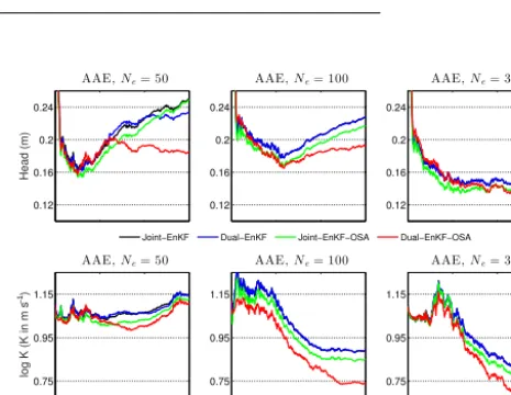
and 300, and we fix the period of the observations to half a day, the number of wells to nine (Fig. 3, left observation network), and the measurement error standard deviation to 0.50 m. We plot the resulting AAE time series of the state and parameters in Fig. 4. As shown, the performance of the joint EnKF, dual EnKF, joint EnKFOSA, and dual EnKFOSA
improves as the ensemble size increases, reaching a mean AAE of 0.161, 0.160, and 0.156 m for Ne=300,
respec-tively. The joint EnKF and the dual EnKF exhibit similar behaviors, with a slight advantage for the dual EnKF. As argued by Gharamti et al. (2014a), the dual EnKF is gen-erally expected to produce more accurate results only when large enough ensembles are used. We have tested the joint and the dual EnKFs using 1000 members and found that the dual EnKF is around 9% more accurate in terms of AAE. The proposed dual EnKFOSAprovides the best estimates in
all tested scenarios. The joint EnKFOSAoutperforms the joint
and dual EnKFs, but is about 5 % less accurate than the dual EnKFOSA, especially after the first year of assimilation. On
average, with changing ensemble size, the dual EnKFOSA
Table 3.Mean average ensemble spread (AESP) of the water head and the hydraulic conductivity for three different ensemble sizes. The reported values are given for the joint EnKF, dual EnKF, joint EnKFOSA, and the proposed dual EnKFOSA.
Hydraulic head Conductivity
Ne=50 Ne=100 Ne=300 Ne=50 Ne=100 Ne=300
Joint EnKF 0.123 0.144 0.200 1.076 1.014 0.951 Dual EnKF 0.126 0.145 0.201 1.075 1.016 0.951 Joint EnKFOSA 0.125 0.145 0.201 1.026 0.977 0.908
[image:11.612.125.471.239.312.2]Dual EnKFOSA 0.117 0.141 0.183 1.039 0.907 0.879
Table 4.Filter inbreeding indicator: Ratio of the mean average absolute error (AAE) and mean average ensemble spread (AESP) of the water head and the hydraulic conductivity for three different ensemble sizes. The reported values are given for the joint EnKF, dual EnKF, and the proposed dual EnKFOSA.
Hydraulic head Conductivity
Ne=50 Ne=100 Ne=300 Ne=50 Ne=100 Ne=300
Joint EnKF 1.734 1.680 1.619 1.539 1.507 1.134 Dual EnKF 1.449 1.443 1.360 1.123 1.123 0.834 Dual EnKFOSA 0.805 0.802 0.854 0.793 0.792 0.801
this eventually changes after 6 months beyond which the dual EnKFOSAclearly outperforms the other schemes.
Furthermore, we examined the estimated uncertainties about the forecast estimates by computing the average spread of both the hydraulic head and conductivity ensembles. To do this, we evaluated the time-averaged AESP of both vari-ables and tabulated the results for the three ensemble sizes in Table 3. For all schemes, increasing the ensemble would increase the spread of the hydraulic head ensemble due to the natural variability of the considered subsurface system. In contrast, the AESP conductivity decreases asNeincreases,
probably because of the persistence nature of its prescribed dynamics. The dual EnKFOSAhas the smallest mean AESP
for all cases, suggesting more confidence in the head and conductivity estimates.
One could also exploit the computed AAE and AESP to assess whether the filters suffer from the inbreeding prob-lem. Filter inbreeding occurs when the variance of the state and parameters ensemble is increasingly reduced over time. This may not only deteriorate the quality of the estimated fil-ter error covariance matrices, but also wrongly suggests more confidence in the forecast and strongly limits the filter update by the incoming observation. One standard test for exam-ining inbreeding is to compute the ratio of the AAE to the AESP (Hendricks Franssen and Kinzelbach, 2008). In a well designed assimilation system (that does not suffer from in-breeding) such a ratio should be close to one; in other words, the AAE and AESP are almost of the same order. Examin-ing Fig. 4 and Table 4, the ratio of the AAE to the AESP for the different tested ensemble sizes is, on-average, very close to 1 for all three schemes, as reported in Table 4. This clearly suggests that no filtering inbreeding issues are encountered in
0.12 0.16 0.2 0.24
Head (m)
AAE,Ne= 50
0.12 0.16 0.2 0.24
AAE,Ne= 100
0.12 0.16 0.2 0.24
AAE,Ne= 300
Joint−EnKF Dual−EnKF Joint−EnKF−OSA Dual−EnKF−OSA
0 6 12 18
0.75 0.95 1.15
Time (months)
log K (K in m s )
AAE,Ne= 50
0 6 12 18
0.75 0.95 1.15
Time (months)
AAE,Ne= 100
0 6 12 18
0.75 0.95 1.15
Time (months)
AAE,Ne= 300
–1
Figure 4.AAE time series of the hydraulic head and conductiv-ity using the joint EnKF, dual EnKF, joint EnKFOSA, and dual
EnKFOSA. Results are shown for three scenarios in which
assim-ilation of hydraulic head data are obtained from nine wells every 0.5 days. The three experimental scenarios use 50, 100, and 300 en-semble members with 0.50 m as the measurement error standard deviation.
[image:11.612.311.544.315.495.2]In terms of computational cost, we note that our assimila-tion results were obtained using a 2.30 GHz workstaassimila-tion and four cores for parallel looping while integrating the ensem-ble members. The joint EnKF is the least intensive requiring 70.61 s to perform a year-and-a-half assimilation run using 50 members. The dual EnKF and dual EnKFOSA, on the other
hand, require 75.37 and 77.04 s, respectively. The dual EnKF is computationally more demanding than the joint EnKF be-cause it includes an additional propagation step of the en-semble members as discussed in Sect. 3.3. Likewise, the pro-posed dual EnKFOSArequires both an additional propagation
step and an update step of the state members. Its computa-tional complexity is thus greater than the joint scheme and roughly equivalent to that of the dual EnKF. Note that in the current setup the cost of integrating the groundwater model is not very significant as compared to the cost of the update step. This is due to the simplified structure of the utilized hy-drological model. This, however, should not hold for large-scale hydrological applications.
5.2 Sensitivity to the frequency of observations
In the second set of experiments, we test the filters’ behavior with different temporal frequency of observations; i.e., the times at which head observations are assimilated. We imple-ment the three filters with 100 members and use data from nine observation wells perturbed with 0.10 m noise.
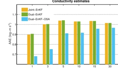
Figure 5 plots the mean AAE of the hydraulic conductivity estimated using the three filters for the six different observa-tions sampling frequencies. The dual and joint EnKFs lead to comparable performances, but the latter performs slightly better when data are assimilated more frequently, i.e., every 5 and 3 days. The performance of the proposed dual EnKFOSA,
as seen from the plot, is rather good and its estimates are more consistent with the data than those computed by the other two filters. The best dual EnKFOSAresults are obtained
when assimilating data every 1, 3, and 5 days. The improve-ments over the joint and the dual schemes decrease as obser-vations are sampled less frequently in time. The reason for this is related to the nature of the dual EnKFOSAalgorithm,
which adds a one-step-ahead smoothing to the analyzed head ensemble members before updating the forecast parameters and the state samples. Therefore, the more data are available, the greater the number of applied smoothing steps, and hence the better the characterization of the state and parameters. To illustrate, the smoothing step of the state ensemble en-hances its statistics and eventually provides more consistent state-parameters cross-correlations to better predict the data. When assimilating hydraulic head data on a daily basis, the proposed dual EnKFOSAleads to about 24 % more accurate
conductivity estimates than the joint and dual EnKFs. We have also compared the hydraulic head estimates for different sampling frequencies of observations. Similar to the parameters, the improvements of the dual EnKFOSA
algo-rithm over the other schemes become significant when more
1 3 5 10 15 30
0.7 0.8 0.9 1 1.1
Observation sampling period (days)
AAE (log−m s )
Conductivity estimates
Joint−EnKF Dual−EnKF Dual−EnKF−OSA
[image:12.612.324.528.70.190.2]–1
Figure 5.Mean average absolute errors (AAE) of log-hydraulic conductivity, log(K), obtained using the joint EnKF, dual EnKF, and dual EnKFOSAschemes. Results are shown for six different
scenarios in which assimilation of hydraulic head data are obtained from nine wells every 1, 3, 5, 10, 15, and 30 days. All six experi-mental scenarios use 100 ensemble members and 0.10 m as the mea-surement error standard deviation.
data are assimilated over time. Overall, the benefits of the proposed scheme seem to be more pronounced for the esti-mation of the parameters, probably because the conductivity values at all aquifer cells are indirectly updated using hy-draulic head data, requiring more observations for efficient estimation.
One effective way to evaluate the estimates of the state is to examine the evolution of the reference heads and the forecast ensemble members at various aquifer locations. For this, we plot in Fig. 6 the true and the estimated time-series change in hydraulic head at the assigned monitoring wells as they result from the joint EnKF, dual EnKF, and the dual EnKFOSA. We use 100 ensemble members and assume the
nine data points are available every 5 days. At MW1, the per-formance of the three filters is quite similar and they all suc-cessfully reduce the uncertainties and recover the true evo-lution of the hydraulic head at that location. We note that between the 5th and the 9th month, the dual EnKF seems to underestimate the reference values of the hydraulic head as compared to the other two schemes. At MW2 and MW3, the ensemble spread of all three filters shrinks shortly after the start of assimilation, but remains larger than those at MW1. The proposed dual EnKFOSAwell recovers the reference
tra-jectory at MW2 and MW3. The ensemble head values ob-tained using the joint and the dual EnKFs at MW2 are less accurate. Furthermore, the joint and the dual EnKF ensemble members tend to underestimate the reference hydraulic head at MW3 over the first 6 months of assimilation. Beyond this, there is a clear overestimation of the head values, especially by the dual EnKF, up to the end of the first year.
5.3 Sensitivity to the number of observations
num-Figure 6. Reference (dashed) and predicted (solid) hydraulic head evolution at monitoring wells MW1, MW2, and MW3. Results are obtained using the joint EnKF and the dual EnKFOSAschemes with 100 members, 5 days as sampling period, nine observation wells, and 0.10 m of measurement noise.
0 6 12 18
0.1 0.15 0.2
Time (months)
AAE (m)
Hydraulic head estimates
Joint−EnKF, p = 15
Dual−EnKF, p = 15
Dual−EnKF−OSA, p = 15
Joint−EnKF, p = 25
Dual−EnKF, p = 25
Dual−EnKF−OSA, p = 25
0 6 12 18
0.8 1 1.2
Time (months)
AAE (log−m s )
Conductivity estimates
[image:13.612.128.469.65.354.2]–1
Figure 7.Time series of AAE of hydraulic head (left panel) and conductivity (right panel) using the joint EnKF, dual EnKF, and dual EnKFOSAschemes. Results are shown for two scenarios in which assimilation of hydraulic head data are obtained from 15 and 25 wells
(uniformly distributed throughout the aquifer domain) every 5 days. The four experimental scenarios use 100 ensemble members and 0.10 m as the measurement error standard deviation. The number of wells is denoted byp.
bers of observation wells inside the aquifer domain. We thus compare our earlier estimates resulting from only nine wells, 5 days sampling period, and 0.10 m measurement error stan-dard deviation with a new set of estimates resulting from more dense observational networks with 15, 25, and 81 wells. Figure 7 plots the time-series curves of the AAE as they
[image:13.612.131.467.413.564.2]Figure 8.Spatial maps of the reference, initial and recovered en-semble means of hydraulic conductivity using the joint EnKF, dual EnKF, and dual EnKFOSAschemes. Results are shown for a
sce-nario in which assimilation of hydraulic head data is obtained from nine wells every 5 days. This experiment uses 100 ensemble mem-bers and 0.10 m as the measurement error standard deviation.
forecast errors for conductivity than does the dual EnKF (and joint EnKF) with 81 data points. Likewise when assimilating head data from 15 and 25 wells, the proposed algorithm out-performs the joint and dual EnKFs and yields more accurate hydraulic head estimates by the end of the simulation win-dow.
To further assess the performance of the filters we analyze the spatial patterns of the estimated fields. To do so, we plot and interpret the ensemble mean of the conductivity as it re-sults from the three filters using nine observation wells. We compare the estimated fields after 18 months (Fig. 8) with the reference conductivity. As can be seen, the joint and the dual EnKFs exhibit some overshooting in the southern (low conductivity) and central regions of the domain. In contrast, the dual EnKFOSAbetter delineates these regions and further
provides reasonable estimates of the low conductivity area in the northwest part of the aquifer. In general and for all tested schemes, the estimated conductivity field does not capture very well the spatial variability of the reference field. This is due to the large model errors imposed on the recharge and pumping rates during the forecasts. This limits the efficiency of the assimilation system, especially with the recovery of small-scale conductivity structures, but also allows for more straightforward assessment of the different techniques.
Observational error (m)
0.05 0.1 0.15 0.2 0.25 0.3 0.5 1 2 3
Mean AAE (log-m s )
0.8 0.85 0.9 0.95 1 1.05
1.1 Conductivity estimates
Joint-EnKF
Dual-EnKF
Dual-EnKF-OSA
–1
Figure 9.Mean AAE of the hydraulic conductivity using the joint EnKF, dual EnKF, and dual EnKFOSAschemes. Results are shown
for 10 different scenarios in which assimilation of hydraulic head data is performed using nine wells with measurement error standard deviations of 0.05, 0.10, 0.15, 0.20, 0.25, 0.3, 0.5, 1, 2, and 3 m. The four experimental scenarios use 100 ensemble members and 5 days as sampling period. Thexaxis is displayed in log scale.
5.4 Sensitivity to measurement errors
In the last set of sensitivity experiments, we fix the number of wells to nine, the sampling period to 5 days, and test with different standard deviations of measurement error to perturb the observations. We plot the results of 10 different obser-vational error scenarios in Fig. 9 and compare the conduc-tivity estimates obtained using the joint EnKF, dual EnKF, and the dual EnKFOSA. In general, the performance of the
filters appears to degrade as the observations are perturbed with a larger degree of noise. All three filters exhibit similar performances with large observational error; i.e., 1, 2, and 3 m. This can be expected because larger observational er-rors decrease the impact of data assimilation, and may reduce the estimation process to a model prediction only. The plot also suggests that the estimates of the dual EnKFOSA with
0.30 m measurement error standard deviation are better than those of the joint and the dual EnKFs with 0.10 m error. With 0.10 m measurement error standard deviation, the estimate of the dual EnKFOSAis also approximately 12 % better.
Finally, we investigated the time evolution of the ensem-ble variance of the conductivity estimates as they result from the dual EnKF and the dual EnKFOSAwith 0.10 m
[image:14.612.328.525.66.241.2]to-Initial uncertainties
Distance (km)
0 0.25 0.5
Distance (km)
0 0.5 1
0 0.02 0.04 0.06 0.08 0.1
After 6 months
0 0.25 0.5
Dual-EnKF
0 0.5 1
After 18 months
0 0.25 0.5 0
0.5 1
0 0.25 0.5
Dual-EnKF-OSA
0 0.5 1
0 0.25 0.5 0
[image:15.612.310.546.64.273.2]0.5 1
Figure 10.Left panel: ensemble variance map of the initial conduc-tivity field. Right sub-panels: ensemble variance maps of estimated conductivity after 6 and 18 month assimilation periods using the dual EnKF and the proposed dual EnKFOSA schemes. These
re-sults are obtained with 100 members, 5 days of sampling period, nine observation wells, and 0.10 m as measurement noise.
wards the north edges than the dual EnKF, which in turn helps increase the weight of the observations in this area. 5.5 Prediction capability assessment
To further assess the system performance in terms of pa-rameters retrieval, we have integrated the model in predic-tion mode (without assimilapredic-tion) for an addipredic-tional period of 18 months starting from the end of the assimilation period. We plot in Fig. 11, using the final estimates of the conduc-tivity as they result from the three filters (after 18 months), the time evolution of the hydraulic head at the CW. The en-semble size is set to 100, sampling period is 1 day, number of data wells is 25, and measurement noise is 0.5 m. The refer-ence head trajectory at the CW decreases from 17.5 to 16.9 m in the first 2 years, and then slightly increases to 17.2 m in the rest of the years. The forecast ensemble members of the joint EnKF at this CW fail to capture to reference trajectory of the model. This is due to the large measurement noise imposed on the head data. The dual EnKF performs slightly better and predicts hydraulic head values that are closer to the reference solution. The performance of the dual EnKFOSA, as shown,
is the closest to the reference head trajectory and, moreover, one of the forecast ensemble members successfully captures the true head evolution. We further plot the absolute bias of the hydraulic head during the prediction phase, i.e., after 1.5 years, using the three filtering schemes. As shown, the bias in the joint EnKF reaches about 0.6 m after 3 years. On the other hand, the dual EnKFOSAand, to a lesser extent, the
[image:15.612.51.286.66.265.2]dual EnKF, clearly lead to more accurate long-term forecasts
Figure 11.Reference (dashed) and predicted (solid) hydraulic head evolution at the control well: CW. Results are obtained using the joint EnKF, dual EnKF, and the dual EnKFOSA schemes with 100 members, 1 day as sampling period, 25 observation wells, and 0.50 m of measurement noise. The last 18 months are purely based on the forecast model prediction with no assimilation of data. In the bottom-right subplot, the absolute bias of hydraulic head is eval-uated for all schemes during the prediction phase only (i.e., after 1.5 years).
with smaller bias in the resulting hydraulic head estimates. A similar tests was also conducted at other locations in the aquifer, all resulting in similar conclusions.
Finally, in order to demonstrate that our results are sta-tistically robust, 10 other test cases with different reference conductivity and heterogeneous recharge maps were investi-gated. In each of these cases, we sampled the reference fields by varying the variogram parameters, such as variance,xand
TC1 TC2 TC3 TC4 TC5 TC6 TC7 TC8 TC9 TC10
Mean AAE (log-m s )
0.7 0.8 0.9 1 1.1 1.2 1.3 1.4
1.5 Conductivity estimates for different test cases
Joint-EnKF
Dual-EnKF
Dual-EnKF-OSA
[image:16.612.51.284.66.160.2]–1
Figure 12.Performance of the joint/dual EnKF and the proposed dual EnKFOSAschemes in 10 different test cases (TC1, TC2, etc.).
Mean AAE of the conductivity estimates are displayed. These re-sults are obtained with 100 members, 3 days of sampling period, nine observation wells, and 0.10 m as measurement noise.
6 Conclusions
We presented a one-step-ahead smoothing-based dual en-semble Kalman filter (dual EnKFOSA) for state-parameter
es-timation of subsurface groundwater flow models. The dual EnKFOSAis derived using a Bayesian probabilistic
formula-tion combined with two classical stochastic sampling prop-erties. It differs from the standard joint EnKF and dual EnKF in the fact that the order of the time-update step of the state (forecast by the model) and the measurement-update step (correction by the incoming observations) is inverted. Com-pared with the dual EnKF, this introduces a smoothing step to the state by future observations, which seems to provide the model, at the time of forecasting, with better and rather physically consistent state and parameters ensembles.
We tested the proposed dual EnKFOSA on a conceptual
groundwater flow model in which we estimated the hydraulic head and spatially variable conductivity parameters. We con-ducted a number of sensitivity experiments to evaluate the accuracy and the robustness of the proposed scheme and to compare its performance against those of the standard joint and dual EnKFs. The experimental results suggest that the dual EnKFOSA is more robust, successfully estimating
the hydraulic head and the conductivity field under differ-ent modeling scenarios. Sensitivity analyses demonstrate that when more observations are assimilated, the dual EnKFOSA
becomes more effective and significantly outperforms the standard joint and dual EnKF schemes. In addition, when using a sparse observation network in the aquifer domain, the accuracy of the dual EnKFOSA estimates is better
pre-served, unlike the dual EnKF, which seems to be more sen-sitive to the number of hydraulic wells. Moreover, the dual EnKFOSAresults are shown to be more robust against
obser-vation noise. On average, the dual EnKFOSA scheme leads
to around 10 % more accurate state and parameter solutions than those resulting from the standard joint and dual EnKFs. The proposed scheme is easy to implement and only re-quires minimal modifications to a standard EnKF code. It is further computationally feasible, requiring only a marginal increase in the computational cost compared to the dual
EnKF. This scheme should therefore be beneficial to the hy-drology community given its consistency, high accuracy, and robustness to changing modeling conditions. It could serve as an efficient estimation tool for real-world problems, such as groundwater, contaminant transport, and reservoir moni-toring, in which the available data are often sparse and noisy. Potential future research includes testing the dual EnKFOSA
with realistic large-scale groundwater, contaminant transport and reservoir monitoring problems. Furthermore, combining the proposed state-parameter estimation scheme with other iterative and hybrid ensemble approaches may be a promis-ing direction for further improvements.
7 Data availability
Appendix A: Some useful properties of random sampling
The following classical results of random sampling are ex-tensively used in the derivation of the ensemble-based filter-ing algorithms presented in this paper.
Property 1 (Hierarchical sampling; Robert, 2007). Assum-ing that one can sample from p(x1) and p(x2|x1), then a
sample,x∗2, fromp(x2)can be drawn as follows:
1. x∗1∼p(x1),
2. x∗2∼p(x2|x∗1).
Property 2 (conditional sampling; Hoffman and Ribak, 1991). Consider a Gaussian pdf, p(x,y), withPxy andPy
denoting the cross-covariance ofxandyand the covariance of y, respectively. Then a sample, x∗, fromp(x|y), can be
drawn as follows: 1. (ex,ey)∼p(x,y), 2. x∗=
ex+PxyP
−1 y [y−ey].
Appendix B: Sampling of the posterior transition pdf We show here that the samples, ex(m)n (xn−1, θ ), given in
Eq. (32), are drawn from the a posteriori transition pdf,
p(xn|xn−1, θ, yn). Lets start by showing how Eqs. (30)–
(31) are obtained. According to Eq. (15), on can show that the members,eξ
(m)
n (xn−1,θ ), given by Eq. (30), are samples
from the transition pdf, p(xn|xn−1,θ )=Nxn(Mn−1(xn−1, θ ),Qn−1). Furthermore, one may use Property 1 in Eq. (22),
which is recalled here,
p (yn|xn−1, θ )=
Z
p (yn|xn)
| {z }
Nyn(Hnxn,Rn)
p (xn|xn−1, θ )
| {z }
≈ n
eξ (m) n (xn−1,θ)
oNe
m=1
dxn, (B1)
to obtain the members,ey(m)n (xn−1,θ ), given by Eq. (31); such
members are, indeed, samples fromp(yn|xn−1,θ ).
Now, using the samples eξ (m)
n (xn−1, θ ) of p(xn|xn−1,
θ )=p(xn|xn−1,θ,y0:n−1)and the samplesey (m)
n (xn−1,θ )of
p(yn|xn−1,θ )=p(yn|xn−1,θ,y0:n−1), one can apply
Prop-erty 2 to the joint pdf,p(xn,yn|xn−1,θ,y0:n−1), assuming
it is Gaussian, to show that the samplesex(m)n (xn−1,θ ), given
in Eq. (32), are drawn from the a posteriori transition pdf,