Performance and robustness of probabilistic river forecasts computed with quantile regression based on multiple independent variables

Performance and robustness of probabilistic

river forecasts computed with quantile regression

based on multiple independent variables

F. Hoss and P. S. Fischbeck

Carnegie Mellon University, Department of Engineering & Public Policy, 5000 Forbes Avenue, Pittsburgh, PA 15213, USA Correspondence to: F. Hoss ([email protected])

Received: 28 August 2014 – Published in Hydrol. Earth Syst. Sci. Discuss.: 14 October 2014 Revised: 28 July 2015 – Accepted: 27 August 2015 – Published: 25 September 2015

Abstract. This study applies quantile regression (QR) to pre-dict exceedance probabilities of various water levels, includ-ing flood stages, with combinations of deterministic fore-casts, past forecast errors and rates of water level rise as independent variables. A computationally cheap technique to estimate forecast uncertainty is valuable, because many national flood forecasting services, such as the National Weather Service (NWS), only publish deterministic single-valued forecasts. The study uses data from the 82 river gauges, for which the NWS’ North Central River Forecast Center issues forecasts daily. Archived forecasts for lead times of up to 6 days from 2001 to 2013 were analyzed. Be-sides the forecast itself, this study uses the rate of rise of the river stage in the last 24 and 48 h and the forecast error 24 and 48 h ago as predictors in QR configurations. When compared to just using the forecast as an independent vari-able, adding the latter four predictors significantly improved the forecasts, as measured by the Brier skill score and the continuous ranked probability score. Mainly, the resolution increases, as the forecast-only QR configuration already de-livered high reliability. Combining the forecast with the other four predictors results in a much less favorable performance. Lastly, the forecast performance does not strongly depend on the size of the training data set but on the year, the river gauge, lead time and event threshold that are being forecast. We find that each event threshold requires a separate config-uration or at least calibration.

1 Introduction

River-stage forecasts are no crystal ball; the future remains uncertain. The past has shown that unfortunate decisions have been made, because of users’ unawareness of the mag-nitude of potential forecast errors (Pielke, 1999; Morss, 2010). For many users, such as emergency managers, fore-casts are most important in extreme situations, such as droughts and floods. Unfortunately, it is exactly in those sit-uations that forecasts are the most uncertain, i.e., forecast er-rors are the largest, due to the infrequency and the subsequent scarcity of data.

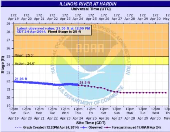
Currently, the National Weather Service (NWS) does not routinely publish uncertainty information along with their deterministic short-term river-stage forecast (Fig. 1). Given the many sources and complexity of uncertainty and the lack-ing user experience, it is easy to see how forecast users find it difficult to estimate the forecast error. Additionally, users might only experience such an event once or twice in their lifetime, so that they have no experience as to what extent they can rely on forecasts in such situations. Including un-certainty in river forecasts would therefore be valuable, just as has been recommended for weather forecasts in general (e.g., National Research Council, 2006). Hopefully, decision-makers would then consider the whole bandwidth of possible future water levels, rather than focusing on the best estimate that is currently being published.

Figure 1. Deterministic short-term weather forecast in 6 h intervals as published by the NWS for Hardin, IL, on 24 April 2014 (source: http://water.weather.gov/ahps2/hydrograph.php?wfo=lsx&gage=hari2).

of uncertainty in a lumped fashion. Both approaches have their advantages and disadvantages. When sources of uncer-tainty are modeled separately, their different characteristics can be taken into account (e.g., some sources of uncertainty depend on lead time, while others do not). Consequently, the approach addressing the major sources of output uncertainty is likely to result in better performing, more parsimonious model configurations. On the downside, this approach is ex-pensive to develop, maintain and run. The alternative, i.e., the lumped quantification of uncertainties, is a less demanding in development and computation runtime but glosses over many of the finer details of uncertainties (Regonda et al., 2013).

Most previously developed post-processors to generate probabilistic forecasts share the overall setup but differ in their implementation. Independent variables such as the fore-casted and observed river stage, river flow or precipitation, and previous forecast errors are used to predict the forecast error, conditional probability distribution of the forecast er-ror or other measures of uncertainty for various lead times (e.g., Kelly and Krzysztofowicz, 1997; Montanari and Brath, 2004; Montanari and Grossi, 2008; Regonda et al., 2013; Seo et al., 2006; Solomatine and Shrestha, 2009; Weerts et al., 2011). These techniques differ in a number of ways, includ-ing their sub-settinclud-ing of data and the output metric. Please see Regonda et al. (2013) and Solomatine and Shrestha (2009) for a summary of each technique.

The National Weather Service has chosen to quantify the most significant sources of uncertainty using ensemble

tech-niques (Demargne et al., 2013). The NWS has developed the Hydrologic Ensemble Forecast Service (HEFS) to be able to provide short-term and medium-term probabilistic forecasts (Demargne et al., 2013). HEFS includes a post-processor, the Hydrologic Ensemble Post-Processor (EnsPost). It mod-els the hydrological uncertainty by estimating the probabil-ity distribution for each of the ensemble members which have been produced with varying input to account for input uncertainty (NWS-OHD, 2013). The Experimental Ensem-ble Forecast Service (XEFS) additionally features the more parsimonious Hydrologic Model Output Statistics (HMOS) streamflow ensemble processor, which estimates the total uncertainty (input and hydrological uncertainty) of single-valued streamflow forecasts based on conditional probability distributions (US Department of Commerce/NOAA, 2012).

deterministic forecasts and the corresponding forecast errors into the Gaussian domain using normal quantile transforma-tion (NQT) to account for heteroscedasticity. Building on the Weerts et al. (2011) study, López López et al. (2014) com-pare different configurations of QR with the forecast as the only independent variable, including configurations without NQT and preventing the crossing of quantiles. They found that no configuration was consistently superior for a range of forecast quality measures (López López et al., 2014).

This paper combines elements of the studies mentioned above. In some aspects, our approach differs from those three studies. We predict the exceedance probabilities of flood stages rather than uncertainty bounds. Additionally, we are fortunate to have a much larger data set than the three earlier studies, consisting of archived forecasts for 82 river gauges covering 11 years. Furthermore, we introduce additional pre-dictors, as was suggested by López López et al. (2014). This study does not add to the mathematical technique of quantile regression itself.

The proposed QR approach is similar to the HMOS ap-proach, but it differs in the following ways. First, HMOS uses ordinary linear regression instead of quantile regres-sion. Second, the QR method uses the single-valued forecast, rates of rise and past forecast errors as independent variables, while HMOS includes recently observed and current flows and quantitative precipitation forecasts (QPFs) as predictors. Third, in this paper, QR models are built for a number of event thresholds, whereas HMOS develops models for sub-sets of forecasted streamflows (Regonda et al., 2013).

Identifying the best-performing set of independent vari-ables is central to this paper. All possible combinations of the following predictors have been studied: forecast, the rate of rise of water levels in past hours, and the past forecast er-rors. Additionally, the robustness of the resulting QR config-urations across different sizes of training data sets, locations, lead times, water levels, and forecast year has been assessed. The paper is structured as follows. The Data section de-scribes the used data and reviews the overall forecast error for the data set. The Method section introduces quantile regres-sion and the performance measures, and discusses the per-formed analyses. The Results describes the results of identi-fying the best-performing set of independent variables. Addi-tionally, it discusses the robustness of the studied QR config-urations. The fourth and last section presents the conclusions and proposes further research ideas.

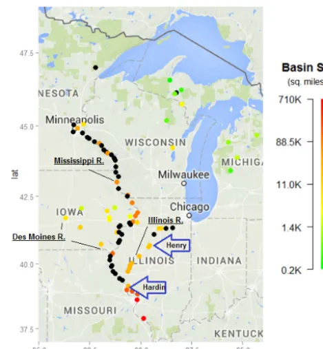
Figure 2. River gauges for which the North Central River Forecast Center publishes forecasts daily. Henry (HYNI2) and Hardin (HARI2) are indicated with arrows. For gauges indicated by black dots the basin size is missing. The color scale for basin size in square miles is logarithmic.

2 Data

The NWS’s daily short-term river forecasts predict the stage height in 6 h intervals for up to 6 days ahead (20 6 h inter-vals). When floods occur and more information is needed, the local river forecast center (RFC) can decide to publish river-stage forecasts more frequently and for more locations. Welles et al. (2007) provides a detailed description of the forecasting process.

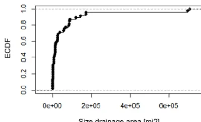
Figure 3. Empirical cumulative density function (ecdf) of sizes of drainage area for the river gauges that are being forecasted daily by the NCRFC.

Two river gauges serve as an illustration for the points made throughout this paper. These two gauges were chosen to capture different but representative conditions. Hardin, IL, is just upstream of the confluence of the Illinois River and the Mississippi River (Fig. 2). Therefore, it can experience back-watering, when the high water levels in the Mississippi River prevent the Illinois River from draining. Henry, IL, is located

∼200 mi upstream of Hardin, having a difference in eleva-tion of∼25 ft. The Illinois River is∼330 mi long (Illinois Department of Natural Resources, 2011), draining an area of

∼13 500 mi2at Henry (USGS, 2015a) and∼28 700 mi2at Hardin (USGS, 2015b). The number of case studies has been limited to two because of computation time.

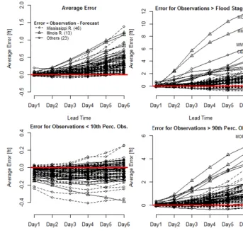
In general, the NCRFC’s forecasts are well calibrated across the entire data set. The average error, defined as ob-servation minus the forecast, is zero for most gauges (Fig. 4). For lead times longer than 3 days, a slight underestimation by the forecast is noticeable. By a lead time of 6 days this un-derestimation averages 0.41 ft (Figs. 4a, 5). Extremely low water levels, defined as below the 10th percentile of ob-served water levels, are also well calibrated (Figs. 4b, 5). However, when considering higher water levels the picture changes. When only observations exceeding the 90th per-centile of all observations are considered, the underestima-tion becomes more pronounced, averaging 0.29 ft for 3 days of lead time and 1.14 ft for 6 days of lead time (Figs. 4c, 5). When only looking at observations that exceeded the minor flood stages corresponding to each gauge, the underestima-tion averages 0.45 ft for 3 days of lead time and 1.51 ft for 6 days of lead time (Figs. 4d, 5). However, some gauges, such as Morris (MORI2), Marseilles Lock/Dam (MMOI2) – both on the Illinois River – and Marshall Town on the Iowa River (MIWI4) experience average errors of 5–12 ft for water levels higher than the minor flood stage. The gauges MORI2 and MMOI2 are upstream of a dam. It is possible that the forecasts performed so poorly there because the dam operators deviated from the schedules that they provide the river forecast centers to base their calculations on. In sum, predicting the forecast error distribution as is done in this

paper has much added value for forecast users, because the forecast error can amount to several feet.

3 Method

QR is used to estimate the distribution of river-stage forecasts for each forecast point in time and location. This information can be published in a number of formats to suit the needs of the forecast users. Wood et al. (2009) and Weerts et al. (2011) chose to study confidence intervals. A confidence interval is the range between two points on the estimated forecast distri-bution, e.g., between the 10th and 90th percentiles. Our pa-per differs in that our output is the probability of exceeding a flood stage. A flood stage and the corresponding probabil-ity of it being exceeded are represented by a single point on the estimated forecast distribution. Assessing forecast per-formance for a single point rather than for two points on the estimated distribution allows for scrutinizing forecast perfor-mance more closely, not least because the method is not nec-essarily equally successful in both tails of the distribution.

In the following, quantile regression itself and the analysis to identify the best-performing set of independent variables are explained.

3.1 Quantile regression

In the context of river forecasts, linear quantile regression has been used to estimate the distribution of forecast errors as a function of the forecast itself. Weerts et al. (2011) summarize this stochastic approach as follows: “[It] estimates effective uncertainty due to all uncertainty sources. The approach is implemented as a post-processor on a deterministic forecast. [It] estimates the probability distribution of the forecast error at different lead times, by conditioning the forecast error on the predicted value itself. Once this distribution is known, it can be efficiently imposed on forecast values.”

Quantile regression was first introduced by Koenker (2005) and Koenker and Bassett (1978). It is different from ordinary least square regression in that it predicts percentiles rather than the mean of a data set. Koenker and Machado (1999, p. 1305) and Alexander et al. (2011) demonstrate that studying the coefficients and their uncertainty for different percentiles generates new insights, especially for non-normally distributed data.

López López et al. (2014) did not find that the quantile regression method produces better forecasts if the variables are subject to NQT beforehand, as was practiced by Weerts et al. (2011). We chose not to apply NQT, because four of five of our independent variables are already approximately normally distributed, only the forecast itself is not.

Figure 4. Forecast error for 82 river gauges that the NCRFC publishes daily forecasts for. In counterclockwise direction starting at the top left: (a) average error; (b) error on days that the water level did not exceed the 10th percentile of observations; (c) error on days that the water level exceeded the 90th percentile of observations; (d) error on days that the water level exceeded minor flood stage.

other, a fixed-effects model is implemented below a certain forecast value. Weerts et al. (2011) give a detailed mathe-matical description for applying QR to river forecasts. De-tailed instructions to perform NQT can be found in Bogner et al. (2012). Mathematically, the approach is formulated as follows (with and without NQT).

Equation (1): QR configuration with NQT, with per-centiles of the forecast error as the dependent variable and the one independent variable, both transformed into the nor-mal domain.

Fτ(t )=fcst(t )+NQT−1 " _I

X

i

ai,τ·VNQT,i(t )+bτ #

(1) Equation (2): QR configuration without NQT, with per-centiles of the forecast error as the dependent variable and multiple independent variables.

Fτ(t )=fcst(t )+ I X

i

ai,τ·Vi(t )+bτ, (2) where Fτ(t ) is the estimated forecast associated with per-centileτ and timet, fcst(t) is the original forecast at timet,

Vi(t )is the independent variablei(e.g., the original forecast) at timet,Vi;NQT(t )is the independent variableItransformed

by NQT at timet andai,τ andbτ are configuration coeffi-cients.

The second part of the equations stands for the error esti-mate based on the quantile regression configuration for each error percentileτ and lead time. In Eq. (1), used by Weerts et al. (2011), this estimation was executed in the Gaussian do-main using only the forecast as independent variable. Our study mainly uses Eq. (2), i.e., it does not transform the predictors and the predictand. All quantile regressions were done using the command rq() in the R package “quantreg” (Koenker, 2013).

3.2 Verification measures

Figure 5. Empirical cumulative distribution function (ecdf) of forecast error at 82 river gauges for six lead times. Vertical lines show the median forecast error of the corresponding subset.

a number of measures to assess configuration performance, e.g., the Brier skill score (BSS), the mean continuous ranked probability (skill) score (CRPSS), the relative operating char-acteristic (ROC), and reliability diagrams to compare QR configurations.

We focus on the BSS – first introduced by Brier (1950) – to assess QR configurations for three reasons. First, to be able to determine the best set of predictors it is easiest to choose a single measure. Second, the BSS allows us to study fore-cast performance at individual event thresholds. Third, out of the available measures, the Brier score is attractive because it can be decomposed into two different measures of forecast quality (see Eq. 3): reliability and resolution. The third com-ponent is uncertainty. This type of uncertainty describes the uncertainty inherent in an event caused by natural variabil-ity. It is narrower than forecast uncertainty, because the latter additionally includes the uncertainty that is caused by imper-fections of the forecast model, i.e., the variables that could explain some of the uncertainty have not been identified or correctly parameterized yet. In sum, the BS’ uncertainty term is not subject to the forecast quality. Equation 3 gives the

definition of the (decomposed) Brier score (e.g., Jolliffe and Stephenson, 2012; Wikipedia, 2014; WWRP/WGNE, 2009). Equation (3): Brier score decomposed into three terms: re-liability, resolution and uncertainty.

BS= 1

N K X

k=1

nk(fk−ok)2−

| {z }

Reliability

1 N

K X

k=1

nk(ok−o)2+

| {z }

Resolution

o(1−o)

| {z } Uncertainty

= 1

N T X

t=1

(ft−ot)2, (3)

Figure 6. Theory behind Brier skill score illustrated for an imaginary forecast (red line): (a) reliability and resolution, (b) skill. In (a), the area representing reliability should be as small as possible and for resolution as large as possible. The forecast has skill (BSS>0), i.e., performs better than the reference forecast, if it is inside the shaded area in (b). Ideally, the forecast would follow the diagonal (BSS=1) (adapted from Hsu and Murphy, 1986; Wilson, 2014).

The Brier score pertains to binary events, e.g., the ex-ceedance of a certain river stage or flood stage. Reliability compares the estimated probability of such an event with its actual frequency. For example, perfect reliability means that on 60 % of all days for which it was predicted that the water level would exceed flood stage with a 60 % probabil-ity, it actually does so. The reliability curve for the forecast representing perfect reliability would follow the diagonal in Fig. 6, i.e., the area in Fig. 6a representing reliability would equal zero (Jolliffe and Stephenson, 2012; Wikipedia, 2014; WWRP/WGNE, 2009).

Resolution measures the difference between the predicted probability of an event on a given day and the historically observed average probability. For example, imagine a gauge where flood stage has historically been exceeded on 5 % of the days in a year. If every day at that gauge the probability of exceeding flood stage is forecasted to be 5 %, the reso-lution of those forecasts would be zero. After all, the dif-ference between the predicted frequency and the historical average is zero. So a forecast with higher resolution is bet-ter (e.g., Jolliffe and Stephenson, 2012; Wikipedia, 2014; WWRP/WGNE, 2009). In Fig. 6, the curve for a forecast with good resolution would be steeper than the dashed line that represents the historically observed frequency (clima-tology). It follows that forecasters should strive to maxi-mize the area in Fig. 6a representing resolution. In abso-lute terms, the resolution can never exceed the uncertainty inherent to the river gauge, as represented by the third term in Eq. (3). (e.g., Jolliffe and Stephenson, 2012; Wikipedia, 2014; WWRP/WGNE, 2009).

A forecast performs better than the reference forecast (in this case the historically observed frequency), if it (the red line) is inside the shaded area in Fig. 6b. Then the forecast is said to have “skill”. The BSS equals the Brier Score

nor-malized by the historically observed frequency, i.e., the res-olution and reliability terms are being divided by the uncer-tainty term (Eq. 4). In contrast to the Brier score, this makes the Brier skill score comparable across gauges with differ-ent frequencies of a binary evdiffer-ent. The BSS can range from minus infinity to one. A BSS below zero indicates no skill; the perfect score is one (e.g., Jolliffe and Stephenson, 2012; Wikipedia, 2014; WWRP/WGNE, 2009).

Equation (4) shows the decomposition of the Brier skill score:

BSS=1− BS

o(1−o)= Res o(1−o)−

Rel

o(1−o), (4)

where BSS is the Brier skill score, BS is the Brier score, Res is the resolution, Rel is the Reliability,δis the frequency of binary event occurring andδ(1−δ the climatological vari-ance.

To verify that the results hold up for verification mea-sures other than the BSS, we additionally use the Continuous Ranked Probability Score (CRPS). The BSS assesses fore-cast performance for one point on the forefore-cast distribution, i.e., one event threshold. In contrast, the CRPS, defined by Eq. (5), measures the forecast performance for the forecast distribution as the whole. Therefore, the CRPS cannot detect whether the forecast does better or worse in the tails. Instead, it is a measure of the forecast’s overall performance. The CRPS’ perfect score equals zero (e.g., Jolliffe and Stephen-son, 2012; WWRP/WGNE, 2009).

All measures of forecast quality were computed using the R package “verification” (NCAR, 2014).

CRPS= 1

N N X

n=1

∞

Z

−∞

where CRPS is the continuous ranked probability score,F_nfis the forecast probability distribution (cdf) for thenth forecast case,F_nois the observation fornth forecast case (cdf) andN is the number of forecast cases, i.e., length of time series. 3.3 Choice of independent variables

The challenge is to identify a well-performing QR model with a set of predictors that is both parsimonious and compre-hensive. Wood et al. (2009) found rate of rise and lead time to be informative independent variables. Weerts et al. (2011) achieved good results using only the forecast itself as pre-dictor. Besides these variables, the most obvious predictors to include are the current water levels and those observed 24 and 48 h ago, and the forecast error 24 and 48 h ago (i.e., the difference between the current water level at issue time of the forecast that the error distribution is being predicted for and the forecasts that were produced 24 and 48 h earlier to predict the current water level). Additional potential inde-pendent variables are the water levels observed at gauges up-and downstream at various times, the precipitation upstream of the catchment area, and the precipitation forecast.

Rates of rise and forecast errors were chosen to comple-ment the forecast as independent variables. Therefore, in-stead of using it as an independent variable, separate QR models have been built for each lead time. After all, the best choice of independent variables might depend on lead time. Precipitation and precipitation forecast were not available for this study, because without direct access to the database at the NCDC requesting that data is a very lengthy effort.

Forecasts and observed water levels were readily acces-sible from NCDC databases. Rates of rise and forecast er-rors can be derived from those two. As will be shown in Sect. 4.3, it is mathematically challenging to combine in-dependent variables with different distributions into a joint predictor. Forecast and observed water levels have a skewed distribution, because low water levels occur more frequently than extremely high water levels, while rates of rise and fore-cast errors are approximately normally distributed. Accord-ingly, either forecasts and observations can easily be com-bined into a joint predictor or rates of rise and forecast errors. For this study the latter option was chosen for the following reasons. Observed water levels are systematically included in the NWS forecast model. Assuming a well-defined NWS forecast model, there should be no statistical relationship be-tween forecast error and observed water levels. In compari-son, rates of rise and forecast error are only included in the NWS model at the discretion of the individual forecaster. Therefore, the latter two variables are likely to contribute more information to predicting the distribution of forecast errors than the forecasts and observed water levels. Nonethe-less, forecasts were included as the predictor in this study to demonstrate the difficulty of combining variables with a skewed distribution with normally distributed variables into a joint predictor, and because it served as the only

indepen-dent variable in previous studies (Weerts et al., 2011; López López et al., 2014).

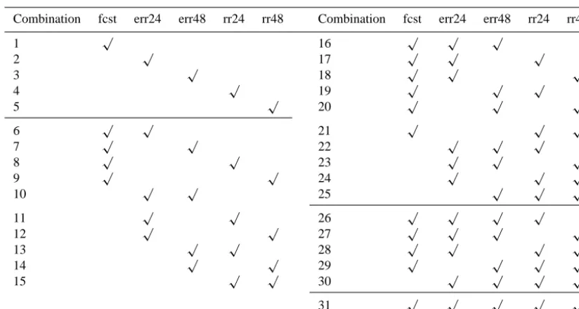
To determine which set of predictors performs best at gen-erating probabilistic forecasts, all 31 possible combinations of the forecast (fcst), the rate of rise in the last 24 and 48 h (rr24, rr48), and the forecast error 24 and 48 h ago (err24, err48) – see Eq. (5) – were tested for 82 gauges that the NCRFC issues forecasts for every morning (Table 1). Based on the Bier skill score, it was determined which joint predic-tor delivers on average the best out-of-sample forecast per-formance for various lead times and water levels.

Equation (6) shows the QR configuration without NQT, with percentiles of the forecast error as the dependent able and varying combinations of the five independent vari-ables. This equation was used to predict the water level dis-tribution for each day at 82 gauges with different lead times. Fτ(t )=fcst(t )+afcst,τ·fcst(t )+arr24,τ·rr24(t )+arr48,τ

·rr48(t )+aerr24,τ·err24(t )+aerr48,τ·err48(t )+bτ (6) whereFτ(t )is the estimated forecast associated with per-centileτ and timet, fcst(t) is the original forecast at timet, rr24(t) and rr48(t) are the rates of rise in the last 24 and 48 h at timet, err24(t) and err48(t) are the forecast errors 24 and 48 h ago (e.g., the original forecast) at timet, andaxx,τ and bτ are the configuration coefficients, forced to be zero if the predictor is excluded from the joint predictor that is being studied.

3.4 Computational process

The final output of the computational process is the proba-bility that a certain water level in the river or flood stage is exceeded on a given day, e.g., “on the day after tomorrow, the probability that the river exceeds 15 ft at location X is 60 %.” This is done in two steps. First, a training data set (first half of the data) is used to define one quantile regression configu-ration for each percentile of the error distributionπ=[0.05, 0.1, 0.15, . . . , 0.85, 0.90, 0.95] and each lead time. The de-pendent variable is the forecast error, i.e., the difference be-tween forecast and observed water level. To recap, depending on configuration (Table 1), the forecast itself, the rates of rise and forecast errors serve as independent variables.

In the second step, these QR configurations are used to predict percentile by percentile the distribution of forecast errors for each day in the verification data set (the second half of the data set). Effectively, for each day in the verification data set, a discrete probability distribution of forecast errors is predicted. Adding the single-valued forecast to the forecast error distribution results in a distribution of predicted water levels. Each estimated percentileπ contributes one point to that distribution.

4 19

5 √ 20 √ √ √

6 √ √ 21 √ √ √

7 √ √ 22 √ √ √

8 √ √ 23 √ √ √

9 √ √ 24 √ √ √

10 √ √ 25 √ √ √

11 √ √ 26 √ √ √ √

12 √ √ 27 √ √ √ √

13 √ √ 28 √ √ √ √

14 √ √ 29 √ √ √ √

15 √ √ 30 √ √ √ √

31 √ √ √ √ √

fcst=forecast; rr24 and rr48=rise rate in the past 24 and 48 h; err24 and err48=forecast error 24 and 48 h ago.

linearly interpolating between the points of the discrete prob-ability distribution that was computed in the previous step. Next, the Brier skill score is determined based on predicted exceedance probability for all days in the verification data set.

To study whether the various combinations of predictors perform equally well for high and low thresholds, these last computational steps (i.e., interpolating to determine the ex-ceedance probability for a certain water level and calculat-ing the BSS) were repeated for eight event thresholds: the 10th, 25th , 75th, and 90th percentiles of observed water lev-els and the four decision-relevant flood stages (action stage, and minor, moderate, and major flood stage) of each gauge. Flood stages indicated when material damage or substantial hinder is caused by high water levels. Therefore, the flood stages correspond with different percentiles at different river gauges.

To determine the best-performing set of independent vari-ables, the entire procedure is repeated for each of the 31 joint predictors in Table 1, thus using a different set of indepen-dent variables each time. The robustness of the technique was tested by analyzing its performance for 82 gauge loca-tions using different lengths of data sets for five different lead times.

4 Results

In total, the BSS for 31 joint predictors (Table 1) across var-ious lead times and event threshold have been compared. Across 82 river gauges, it has been analyzed which joint pre-dictor delivers the best BSSs on average. When informative,

the CRPS has been used as an additional measure of forecast performance.

4.1 Identifying best-performing joint predictors on average

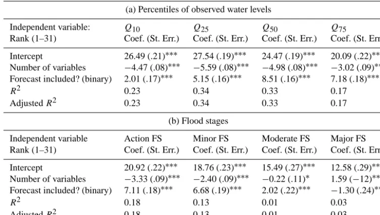
For each river gauge, the combinations have been ranked by BSSs. The best-performing combination was ranked as first, the worst-performing as 31st. It was found that the more independent variables are included in a joint predictor, the higher that set of predictors will rank on average (Fig. 7, Table 2a). Apparently, every additional independent variable does add information. In other words, the future forecast er-ror is a function of rates of rise and past forecast erer-rors. Rising water levels are difficult to anticipate and therefore a common source of forecast error, because precipitation is a major source of input uncertainty. For example, it is never completely certain into which river basin the rain will fall. Additionally, only the expected precipitation for the com-ing 12 h is currently included in forecasts, regardless of lead time. The past forecast errors are a measure of the magni-tude of impact those unanticipated developments are likely to have.

Figure 7. Average rank for each joint predictor for 1–4 days of lead time and two percentiles of observed water levels. Vertical gray lines correspond to the configurations that include the forecast as one of the predictors. Theyaxis is reversed so that an increasing trend indicates increasing performance.

Figure 8. Average rank for each joint predictor for 1–4 days of lead time and the two highest flood stages. Vertical gray lines correspond to the configurations that include the forecast as one of the predictors. Theyaxis is reversed so that an increasing trend indicates increasing performance.

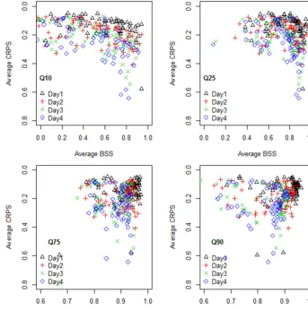
The results hold up when CRPS instead of BSS is used as a measure of forecast performance. The average rank of joint predictors based on CRPS is proportional to the average rank as measured by the BSS previously (Fig. 9). However, scores themselves are not proportional (Fig. 10), because the BSS assesses one point on the estimated distribution, while the CRPS measures the forecast performance for the distribution as a whole. Figure 10 shows that BSS and CRPs correspond well for event thresholdsQ25 andQ75. However, the BSS

indicates that in the tails (Q10, Q90) the forecast does not

perform as well, i.e., despite equally good CRPS scores the BSS varies widely.

4.2 Combining differently distributed variables into a joint predictor

The combinations including the forecast (indicated by gray vertical lines in Figs. 7 and 8) perform significantly better than those that exclude it (Table 2). This disadvantageous impact of the forecast as an independent variable is less pro-nounced for very high or low event thresholds (Table 2a). Including the forecast into the joint predictor is even benefi-cial for major flood stages (Table 2b), when joint predictors with less rather than more variables perform better.

distri-Number of variables −4.47 (.08)∗∗∗ −5.59 (.08)∗∗∗ −4.98 (.08)∗∗∗ −3.02 (.09)∗∗∗ Forecast included? (binary) 2.01 (.17)∗∗∗ 5.15 (.16)∗∗∗ 8.51 (.16)∗∗∗ 7.18 (.18)∗∗∗

R2 0.23 0.34 0.33 0.17

AdjustedR2 0.23 0.34 0.33 0.17

(b) Flood stages

Independent variable Action FS Minor FS Moderate FS Major FS

Rank (1–31) Coef. (St. Err.) Coef. (St. Err.) Coef. (St. Err.) Coef. (St. Err.)

Intercept 20.92 (.22)∗∗∗ 18.76 (.23)∗∗∗ 15.49 (.27)∗∗∗ 12.58 (.29)∗∗∗ Number of variables −3.33 (.09)∗∗∗ −2.40 (.09)∗∗∗ −0.22 (.11)∗ 1.59 (−12)∗∗∗ Forecast included? (binary) 7.11 (.18)∗∗∗ 6.68 (.19)∗∗∗ 2.02 (.22)∗∗∗ −1.30 (.24)∗∗∗

R2 0.18 0.13 0.01 0.03

AdjustedR2 0.18 0.13 0.01 0.03

pvalues:∗∗∗_:<0.001;∗∗_{: 0.01;}∗_{: 0.05; (.): 0.1.}

Figure 10. Comparing the performance of combination 30 (err24, err48, rr24, rr48) as measured by Brier skill score and as measured by the continuous ranked probability score. Each data point corresponds with a gauge at a certain lead time. Since the CRPS’ perfect score equals zero, theyaxis has been reversed.

butions are different. Unlike the dependent variable (fore-cast error), the fore(fore-casts are highly skewed towards the left, because low water levels occur more frequently. Due to its skewed distribution, the forecast becomes a better predictor in a quantile regression predicting a normally distributed de-pendent variable after a NQT transformation, as successfully used by Weerts et al. (2011). Without a transformation into the normal domain, the scatterplot of forecast and forecast error does not show obvious quantile trends (Fig. 11a). After NQT, the percentiles show distinct quantile trends laid out like a fan (Fig. 12a).

In contrast, errors and rise rates are already approximately normally distributed. No quantile trends can be visually de-tected after the other four predictors have been subjected to NQT (Fig. 11b–e). In sum, forecast performance in this study is better without NQT, because four of the five independent variables were approximately normally distributed already. Further research is necessary to reconcile predictors with dif-ferent distributions. Possible solutions could be to define QR configurations for subsets of the transformed dependent and

independent variables or to experiment with subjecting only some but not all predictors to NQT.

4.3 Improvement in forecast performance

Using the best-performing joint predictor at each river gauge gives an upper bound of the BSSs that can be achieved at best. Confirming the Wood et al. (2009) findings, addition-ally including the rates of rise and forecasts errors as in-dependent variables into the QR configuration improves the BSS significantly. Figure 13 illustrates the BSS when using the forecast as the only predictor, as studied by Weerts et al. (2011), while Fig. 14 shows the performance for the best joint predictor at each gauge.

ex-Figure 11. Independent variables plotted against the forecast error for Hardin, IL, with 3 days of lead time. First row: forecast; second row: past forecast errors; third row: rates of rise.

ceedance probabilities of low event thresholds requires much better prediction of the forecast error in feet than for higher event thresholds.

Additionally, Figs. 13–15 show that forecast performance also decreases with increasing lead time, because variables such as rates of rise and past forecast error become propor-tionally less representative with lead time.

Paired t tests for each combination of lead time and event threshold indicate that using the best joint predictor at each gauge increased average BSS across all gauges statisti-cally significantly (Table 3). The performance improves most where forecasts tend to perform worse. The average increase in BSS is largest for extreme water levels, most notably for moderate and major flood stages and for the 10th percentile

of water levels (Table 3). The average increase of BSS for a major flood stage is even larger than one, meaning that fre-quently the method did not have skill before, i.e., negative BSSs. Additionally, predictions with longer lead times ex-perience larger increases in BSS. Compared to using only the forecast as an independent variable, using the best com-binations of forecast, rates of rise and past forecast errors as predictors at each gauge not only increases the mean BSS but also decreases the standard deviation of skill scores across gauges, i.e., performance becomes more consistent (Figs. 13, 14).

Figure 12. Independent variables after transforming into the Gaussian domain plotted against the forecast error for Hardin, IL, with 3 days of lead time. First row: forecast; second row: past forecast errors; third row: rates of rise.

deviation decrease. The improvement is more pronounced for longer lead times (Fig. 16). Moving away from aver-age CRPS, Table 4 reveals that the best joint predictors for high event thresholds (Q75,Q90) do not benefit the average

CRPS. The fact that the average CRPS does not improve im-plies that the best joint predictors for high event thresholds increase forecast performance less for high event thresholds than it worsens performance for low event thresholds. The best joint predictors for low event thresholds (Q10,Q25) do

improve average CRPS, so they must be improving the fore-cast so substantially that the average CRPS increases, even though those best predictors might not perform well for high event thresholds. This is congruent with the finding that av-erage BSS increases much more for percentilesQ10andQ25

than forQ75andQ90, as shown in Table 3. This reinforces

the finding that separate QR models should be configured for individual event thresholds based on the BSS, rather than for the whole distribution based on the CRPS.

The fact that the Brier score can be decomposed into reli-ability, resolution and uncertainty allows for a closer look at which improvements are being achieved by including more predictors than just the forecast. Table 4 summarizes the re-sults of pairedt tests comparing the forecast-only and the best-performing joint predictor for each gauge for the com-ponents of the BSS as well as the CRPS.

(Ta-Q25 0.13 6.06 81 .000 0.15 7.10 81 .000 0.18 9.00 80 .000 0.20 11.35 80 .000

Q₇₅ 0.03 10.19 81 .000 0.05 9.58 81 .000 0.08 11.00 81 .000 0.12 10.80 81 .000

Q90 0.03 8.38 81 .000 0.06 9.33 81 .000 0.10 10.54 81 .000 0.15 11.95 81 .000

Action 0.05 7.76 72 .000 0.14 2.37 73 .010 0.14 5.39 73 .000 0.18 7.30 73 .000

Minor 0.40 2.98 60 .002 0.35 3.37 60 .001 0.37 3.70 60 .000 0.51 4.35 62 .000

Moderate 0.44 2.93 41 .003 0.52 2.94 42 .003 0.81 3.97 45 .000 0.74 5.08 47 .000

Major 1.36 3.00 19 .004 1.84 4.27 22 .000 2.14 4.85 26 .000 1.80 6.01 34 .000

∗_{Df means degrees of freedom.}

Figure 13. BSS for the forecast-only configuration for different lead times and event thresholds. The BSS’ perfect score equals one. A BSS of zero indicates a forecast without skill.

ble 4). Visualizing the improvement in forecast performance for a lead time of 3 days and the 75th percentile threshold (Q75), Fig. 17 illustrates that the forecast-only QR

configu-ration as studied by Weerts et al. (2011) has high reliability (i.e., the reliability is close to zero). So reliability improves statistically significantly for lower water levels (Q10,Q25),

but the magnitude of improvement in reliability is 1 order of magnitude smaller than the improvement in resolution (Ta-ble 4).

4.4 One-size-fits-all approach – Brier skill score Combing these findings, the configurations for the various river gauges can generally be based on the same joint predic-tor of the four independent variables excluding the forecast itself (combination 30). But for extremely high water levels, a configuration specific to each river gauge has to be built in order to achieve high BSSs.

Figure 14. BSS for the best-performing joint predictor at each gauge for different lead times and event thresholds. The BSS’ per-fect score equals one. A BSS of zero indicates a forecast without skill.

Verifying this finding, a one-size-fits-all approach was tested to investigate whether customizing the QR configu-ration to each river gauge would be worth it. The rates of rise in the past 24 and 48 h and the forecast errors 24 and 48 h ago (combination 30 in Table 1) serve as independent vari-ables for this approach. This combination of predictors has been chosen, because it performed well for most gauges (see Sect. 4.1). Furthermore, less important predictors in the com-bination will get small coefficients in the quantile regression. So additional variables are unlikely to do harm but can im-prove the estimates at various stages. The price of opting for a joint predictor with more variables is an increase of the risk of overfitting.

av-Table 4. Results of pairedttests comparing the QR method’s performance with only forecast as predictor and the best-performing combina-tion of five predictors for each river gauge for the Brier score.

Event Lead Brier Brier Reliability Resolution CRPS

threshold time score skill score

Q10

1 day −.012∗∗∗ .20∗∗∗ −.002∗∗∗ .008∗∗∗ −.026*∗∗ 2 days −.014∗∗∗ .25∗∗∗ −.002∗∗∗ .010∗∗∗ −.082∗∗ 3 days −.016∗∗∗ .28∗∗∗ −.002∗∗∗ .012∗∗∗ −.121∗∗∗ 4 days −0.17∗∗∗ .27∗∗∗ −.001∗ .013∗∗∗ −.054

Q25

1 day −.018∗∗∗ .13∗∗∗ −.003∗∗∗ .013∗∗∗ −.028∗∗ 2 days −.023∗∗∗ .16∗∗∗ −.002∗∗∗ .018∗∗∗ −.088∗∗ 3 days −.027∗∗∗ .18∗∗∗ −.003∗∗∗ .021∗∗∗ −.097∗∗ 4 days −.031∗∗∗ .20∗∗∗ −.002∗∗∗ .025∗∗∗ −.475.

Q75

1 day −.005∗∗∗ .03∗∗∗ .000 .011∗∗∗ .342

2 days −.011∗∗∗ .05∗∗∗ −.000. .015∗∗∗ .009

3 days −.016∗∗∗ .08∗∗∗ −.000 .021∗∗∗ .188

4 days −.025∗∗∗ .12∗∗∗ −.000 .028∗∗∗ −.064

Q90

1 day −.003∗∗∗ .03∗∗∗ −.000∗∗ .013∗∗∗ .159 2 days −.005∗∗∗ .06∗∗∗ −.000∗ .015∗∗∗ −.086∗∗

3 days −.010∗∗∗ .10∗∗∗ −.000 .019∗∗∗ .163

4 days −.015∗∗∗ .15∗∗∗ −.000∗ .025∗∗∗ −.075

pvalues:∗∗∗_:<0.001;∗∗_{: 0.01;}∗_{: 0.05; . : 0.1.}

Q75 .003 6.56 81 .000 .004 7.25 81 .000 .005 4.63 81 .000 .004 6.42 81 .000 Q90 .008 7.10 81 .000 .015 4.37 81 .000 .012 5.16 81 .000 .021 1.84 81 .035

Action .024 1.94 72 .028 .031 1.97 73 .026 .039 1.96 73 .027 .022 2.20 73 .016 Minor .023 3.14 60 .001 .028 3.52 60 .000 .021 4.89 60 .000 .023 3.89 62 .000 Moderate .039 4.79 41 .000 .052 6.18 42 .000 .063 4.98 45 .000 .060 4.40 47 .000 Major .245 2.09 19 .025 .212 2.34 22 .014 .234 2.66 26 .007 .375 3.25 34 .001

Figure 16. CRPS for the forecast-only configuration and for the best-performing joint predictor at each gauge for different lead times and event thresholds. The CRPS’ perfect score equals zero.

erage performs statistically significantly not as well as us-ing the best-performus-ing combination of predictors. But the difference in average BSS is small, ranging between 0.003 and 0.075 (Table 5).

However, using the best joint predictors results in a much better performance for major flood stages than the one-size-fits-all approach. The average difference between average BSSs amounts to 0.21–0.38 (Table 5). Given that a BSS for a forecast with skill ranges between one and zero, this is a sub-stantial difference. In sum, the same joint predictor can be used for all river gauges without much loss in performance, except for extremely high water levels.

4.5 Robustness

4.5.1 Minimum length of training data set

Stationarity cannot always be assumed (Milly et al., 2008). River regimes can change through natural processes like

sed-Figure 17. Comparison of the forecast-only QR configuration (i.e., only transformed forecast as independent variables) and us-ing the best-performus-ing joint predictor at each gauge along vari-ous measures of forecast quality: BS, BSS, reliability (Rel), resolu-tion (Res), and CRPS. Lead time of 3 days and 75th percentile of observation levels as threshold.

imentation or human intervention. Those changes can occur gradually or as step changes. This analysis of robustness is meant to determine the minimum length of the training data set to be able to produce skillful forecasts again after a step change using the QR method. Additionally, the analysis is meant to find out to which length the forecaster should limit the training data set when gradual change is occurring. After all, in such a case, each year further in the past is less repre-sentative of the year ahead, so the training data set should be as short as possible.

Figure 18. Brier skill score for various forecast years and various sizes of the training data set across different lead times (colors) and event thresholds (plots) for Hardin, IL (HARI2). The filled-in end point of each line indicates the BSS for the forecast year on thexaxis with 1 year in the training data set. Each point to the left stands for 1 additional training year for that same forecast year.

i.e., the forecasts for 2005 are produced by a model trained on less data than those for 2013. Then, the BSS for that year (e.g., 2005 or 2013) was computed.

Figures 18 and 19 show that at Henry and Hardin it barely matters for the BSS how many years are included in the training data set. This finding is congruent with the fact that Weerts et al. (2011) were able to achieve outstanding results with the QR method using training data sets that were only 2 years long. Only needing short time series to define a skillful QR configuration implies (i) skillful forecasts can be pro-duced not long after a step change and that (ii) the configu-ration parameters can be updated regularly so that gradually changing relationships between predictors, for example, can be taken into account.

4.5.2 Sensitivity analysis

Furthermore, we aim at identifying the factors that impact forecast skill as quantified by the BSS and at generalizing the result regarding training data length described for Hardin and Henry above. To do so, the same analysis as for Hardin

and Henry was repeated for all 82 gauges. Following that, a regression analysis was executed with the BSS as the depen-dent variable and event thresholds (Q10,Q25,Q75,Q90), the

river gauges and forecast years as independent nominal vari-ables, and the lead time (1–4 days) and number of training years as independent ratio variables. This regression is meant to identify the factors to which the forecast performance as measured by the BSS is sensitive to, i.e., which factors sta-tistically significantly impact forecast performance.

The forecast performance was found to vary statistically significantly across all tested dimensions, except the number of training years (Table 6). This results in a very wide range of BSSs (Figs. 13, 14). Accordingly, for the user, it is par-ticularly difficult to know how much to trust a forecast if the performance depends so much on context. Likewise, this is the case for the QR configuration based on the forecast only (not shown).

pre-Figure 19. Brier skill score for various forecast years and various sizes of the training data set across different lead times (colors) and event thresholds (plots) for Henry, IL (HNYI2). The filled-in end point of each line indicates the BSS for the forecast year on thexaxis with 1 year in the training data set. Each point to the left stands for 1 additional training year for that same forecast year.

dict the water levels much more accurately to achieve a sim-ilar forecast performance than for higher water levels, due to the skewed distribution of water levels. In the lower tail, each percentile corresponds with a much shorter span of wa-ter levels than in the upper tail. Using a higher resolution in the lower tail is therefore advisable.

As expected, the BSSs slightly decrease with lead time, because independent variables such as rates of rise and past forecast error gradually become less representative of the days to be forecasted.

Regarding the forecast quality for each forecast year, the regression is slightly biased. The earlier years are included less often in the data set, having on average less years of data in their training data set because, for example, unlike for the year 2013, 10 years of training data were not available for the year 2006. Nonetheless, the regression indicates that 2008 was particularly difficult to forecast and 2012 relatively easy, i.e., they are associated with relatively low and high coefficients respectively (Table 6).

The performance of the forecast additionally depends on the river gauge. The coefficients of the river gauges, included

as factors in the regression, have been excluded from Table 6 for the sake of brevity. Instead, Fig. 20 maps the geographic position of the river gauges with the color code indicating each gauge’s regression coefficient. The coefficient indicates the method’s performance at the particular gauge as com-pared to the average performance. The coefficients are lower and therefore the Brier skill scores are lower for gauges far upstream a river, off the main stream, and those close to con-fluences.

Precipitation is one of the major sources of uncertainty in river forecasting. For example, if rainfall shifts by a few miles it might be raining down in a different river basin. This makes rises in water level difficult to anticipate, making rates of rise such a successful predictor of the distribution of forecast er-rors. However, upstream and close to confluences, rates of rise and past forecast errors perform less well as predictors than elsewhere. This suggests that uncertain expected rainfall constitutes a smaller part of the overall uncertainty.

Figure 20. Geographical position of rivers. Colors indicate the re-gression coefficient of each station with the Brier skill score as de-pendent variable.

associated with the joining river itself, e.g., the uncertain expected rainfall along its course. At upstream gauges, the rates of rise possibly provide less information, because due to smaller basin sizes concentration times are shorter, i.e., water levels rise quicker. In this case, the rise in water level of the past 24 and 48 h may not sufficiently capture rises oc-curring with shorter notice. The argument holds for forecast errors as well. If concentration times are short, the forecast error of 48 h ago is not representative of those in the near future.

5 Conclusions

In this study, QR has been applied to estimate the probabil-ity of the river water level exceeding various event thresh-olds (i.e., 10th, 25th, 75th, and 90th percentiles of observed water levels as well as the four flood stages of each river gauge). It further develops the application of QR for estimat-ing river forecast uncertainty (a) comparestimat-ing different sets of independent variables and (b) testing the technique’s robust-ness across locations, lead times, event thresholds, forecast years and sizes of the training data set.

When compared to the configuration using only the fore-cast, it was found that including rates of rise in the past 24 and 48 h and the forecast errors of 24 and 48 h ago as independent variables improves the performance of the QR configuration, as measured by the Brier skill score. This

con-Table 6. Regression results of sensitivity analysis.

Coefficient SD

Intercept −0.111 0.029 ∗∗∗

Event thresholds ∗∗∗

Q₂₅ 0.584 0.006 ∗∗∗

Q₇₅ 0.852 0.006 ∗∗∗

Q₉₀ 0.805 0.007 ∗∗∗

Forecast years ∗∗∗

2004 −0.259 0.019 ∗∗∗

2005 −0.083 0.017 ∗∗∗

2006 −0.136 0.017 ∗∗∗

2007 −0.123 0.016 ∗∗∗

2008 −0.205 0.016 ∗∗∗

2009 −0.128 0.016 ∗∗∗

2010 −0.141 0.016 ∗∗∗

2011 −0.127 0.016 ∗∗∗

2012 0.048 0.016 ∗∗∗

2013 −0.042 0.016 ∗∗∗

Numbers of years in training data set 0.001 0.001

River gauges ∗∗∗

For the sake of brevity, the 82 river gauges included in the regression as nominal variables have been omitted here.

R2 0.32

AdjustedR2 0.31

pvalues:∗∗∗_:<0.001;∗∗_{: 0.01;}∗_{: 0.05; (.): 0.1.}

firms Wood et al.’s (2009) finding that rate of rise is a valu-able predictor for QR error models. The configuration with the forecast as the only independent variable, as studied by Weerts et al. (2011), produced estimates with high reliability. Including the other four predictors mentioned above mainly increases the resolution.

For extremely high water levels, the combinations of in-dependent variables that perform best vary across stations. On those days, combinations of fewer independent variables perform better than those that include more. The most likely explanation is that QR configurations based on large joint predictors result in overfitting the data. In contrast to these extremely high event thresholds, larger sets of predictors work better than smaller ones for non-extreme and low event thresholds. Additionally, customizing the set of predictors to the event thresholds does not improve the BSS much, except for extremely high event thresholds, i.e., major flood stage.

This study shows the importance of configuring QR mod-els for individual event thresholds rather than using one con-figuration to estimate the whole forecast distribution. The tails are too different to use the same joint predictors and parametrization.

The studied QR configurations are relatively robust to the size of training data set, which is convenient if stationarity cannot be assumed (Milly et al., 2008), a step change in the river regime has occurred or – as is the case for most river forecast centers – only recent forecast data have been archived. However, the performance of the technique de-pends heavily on the river gauge, the lead time, event thresh-old and year that are being forecast. This results in a very wide range of Brier skill scores. This means that the dan-ger remains that forecast users make good experiences with a forecast one year or at one location and assume it is equally reliable in other locations and every year. As is the case with most other forecasts, an indication of forecast uncertainty needs to be communicated alongside the exceedance prob-abilities generated by our approach.

As is the case for many forecasting methods, the stud-ied QR configurations perform less well for longer lead times, extreme event thresholds that are characterized by data scarcity, and for gauges far upstream a river, off the main stream or close to confluences where different factors interact with each other. Additionally, QR configurations underper-form for low event thresholds. Due to the skewed distribution of water levels, forecasts have to perform better in estimating low water levels to achieve the same BSSs as for high event thresholds, because in the lower tail each percentile spans a smaller range of water levels. Using a higher resolution in the lower tail would probably improve the forecast performance for low event thresholds.

6 Future work

This technique can be further developed in several ways to achieve higher Brier skill scores and more robustness. First, more independent variables can be added. Observed precip-itation, the precipitation forecast (i.e., POP – probability of precipitation) and the upstream water levels are promising candidates, because the forecast used in this study includes the precipitation forecast for only the next 12 h. However, currently, the precipitation data and forecasts can only be re-quested in chunks of a month, three chunks per day, from the NCDC’s HDSS Access System. For a period of 12 years, re-questing such data for several weather stations is obviously time consuming, not least because the geographical units of

river should be included as well.

However, note that many hydrological variables have a skewed distribution, so that they cannot readily be combined into a joint predictor with normally distributed variables such as rates of rise and past forecast errors, as used in this study. Future work should focus on reconciling predictors with dif-ferent distributions.

Different approaches of sub-setting the data to improve performance also warrant consideration in boosting the per-formance of the QR method. Particularly, clustering the data by variability seems promising.

Additionally, the studied technique would need to be ver-ified for gauges for which the NCRFC does not publish daily forecasts. Ignorance of the uncertainty inherent in river forecasts has had some of the most unfortunate impacts on decision-making in Grand Forks, ND, and Fargo, ND (Pielke, 1999; Morss, 2010). Both of those stages are discontinuously forecasted NCRFC gauges.

Finally, this paper uses a brute force approach by simply calculating and comparing all possible combinations of inde-pendent variables. A mathematically more challenging step-wise quantile regression would not only be more elegant but would also provide better safeguards against overfitting the data.

Acknowledgements. Many thanks to Grant Weller, who suggested looking into quantile regression to predict forecast errors. We would like to thank the three reviewers for their insightful comments. The paper greatly benefitted from their comments. As to funding, Frauke Hoss is supported by an ERP fellowship of the German National Academic Foundation and by the Center of Climate and Energy Decision Making (SES-0949710), through a cooperative agreement between the National Science Foundation and Carnegie Mellon University (CMU).

Edited by: A. Weerts

References

Alexander, M., Harding, M., and Lamarche, C.: Quantile Regres-sion for Time-Series-Cross-Section-Data, Int. J. Stat. Manage. Syst., 4, 47–72, 2011.

Bogner, K., Pappenberger, F., and Cloke, H. L.: Technical Note: The normal quantile transformation and its application in a flood forecasting system, Hydrol. Earth Syst. Sci., 16, 1085–1094, doi:10.5194/hess-16-1085-2012, 2012.

Demargne, J., Wu, L., Regonda, S. K., Brown, J. D., Lee, H., He, M., Seo, D.-J., Hartman, R., Herr, H. D., Fresch, M., Schaake, J., and Zhu, Y.: The Science of NOAA’s Operational Hydrologic Ensemble Forecast Service, B. Am. Meteorol. Soc., 95, 79–98, doi:10.1175/BAMS-D-12-00081.1, 2013.

Hsu, W. and Murphy, A. H.: The attributes diagram A geometri-cal framework for assessing the quality of probability forecasts, Int. J. Forecast., 2, 285–293, doi:10.1016/0169-2070(86)90048-8, 1986.

Illinois Department of Natural Resources: Aquatic Illinois – Illi-nois Rivers and Lakes Fact Sheets, available at: http://dnr.state. il.us/education/aquatic/aquaticillinoisrivlakefactshts.pdf (last ac-cess: 3 February 2015), 2011.

Jolliffe, I. T. and Stephenson, D. B.: Forecast Verification: A Prac-titioner’s Guide in Atmospheric Science, John Wiley & Sons, doi:10.1002/9781119960003.fmatter/pdf, 2012.

Kelly, K. S. and Krzysztofowicz, R.: A bivariate meta-Gaussian density for use in hydrology, Stoch. Hydrol. Hydraul., 11, 17– 31, doi:10.1007/BF02428423, 1997.

Koenker, R.: Quantile Regression, Cambridge University Press, 2005.

Koenker, R.: quantreg: Quantile Regression, R Package Ver-sion 505, available at: http://CRAN.R-project.org/package= quantreg (last access: 27 August 2014), 2013.

Koenker, R. and Bassett, G.: Regression Quantiles, Econometrica, 46, 30–50, doi:10.2307/1913643, 1978.

Koenker, R. and Machado, J. A. F.: Goodness of Fit and Related Inference Processes for Quantile Regression, J. Am. Stat. Assoc., 94, 1296–1310, doi:10.1080/01621459.1999.10473882, 1999. Leahy, C. P.: Objective Assessment and Communication of

Uncer-tainty in Flood Warnings, 5th Flood Management Conference, 9–12 October 2007, Warrnamboll, 2007.

López López, P., Verkade, J. S., Weerts, A. H., and Solomatine, D. P.: Alternative configurations of quantile regression for estimat-ing predictive uncertainty in water level forecasts for the upper Severn River: a comparison, Hydrol. Earth Syst. Sci., 18, 3411– 3428, doi:10.5194/hess-18-3411-2014, 2014.

Milly, P. C. D., Betancourt, J., Falkenmark, M., Hirsch, R. M., Kundzewicz, Z. W., Lettenmaier, D. P., and Stouffer, R. J.: Sta-tionarity Is Dead: Whither Water Management?, Science, 319, 573–574, doi:10.1126/science.1151915, 2008.

Montanari, A. and Brath, A.: A stochastic approach for assess-ing the uncertainty of rainfall-runoff simulations, Water Resour. Res., 40, W01106, doi:10.1029/2003WR002540, 2004. Montanari, A. and Grossi, G.: Estimating the uncertainty of

hydro-logical forecasts: A statistical approach, Water Resour. Res., 44, W00B08, doi:10.1029/2008WR006897, 2008.

Morss, R. E.: Interactions among Flood Predictions, Decisions, and Outcomes: Synthesis of Three Cases, Nat. Hazards Rev., 11, 83– 96, doi:10.1061/(ASCE)NH.1527-6996.0000011, 2010. National Climatic Data Center: HDSS Access System,

avail-able at: http://cdo.ncdc.noaa.gov/pls/plhas/HAS.FileAppSelect? datasetname=9957ANX, last access: 15 July 2014.

National Research Council: Completing the Forecast: Characteriz-ing and CommunicatCharacteriz-ing Uncertainty for Better Decisions Us-ing Weather and Climate Forecasts, National Academies Press, Washingtion, D.C., available at: http://www.nap.edu/catalog. php?recordid=11699 (last access: 18 September 2014), 2006.

NCAR: Research Application Program, verication: Forecast Verica-tion Utilities, http://CRAN.R-project.org/ (last access: Septem-ber 2015), 2014.

NWS-OHD – National Weather Service, Office of Hydrologic De-velopment: Ensemble Postprocessor (EnsPost) User’s Manual, HEFS Release 0.3.2, available at: http://www.nws.noaa.gov/oh/ hrl/general/HEFS_doc/HEFS-0.3.2EnsPostUsers_Manual.pdf (last access: 22 July 2015), 2013.

Pielke, R. A.: Who Decides? Forecasts and Responsibilities in the 1997 Red River Flood, Appl. Behav. Sci. Rev., 7, 83–101, 1999. Regonda, S. K., Seo, D.-J., Lawrence, B., Brown, J. D., and De-margne, J.: Short-term ensemble streamflow forecasting using operationally-produced single-valued streamflow forecasts – A Hydrologic Model Output Statistics (HMOS) approach, J. Hy-drol., 497, 80–96, doi:10.1016/j.jhydrol.2013.05.028, 2013. Seo, D.-J., Herr, H. D., and Schaake, J. C.: A statistical

post-processor for accounting of hydrologic uncertainty in short-range ensemble streamflow prediction, Hydrol. Earth Syst. Sci. Dis-cuss., 3, 1987–2035, doi:10.5194/hessd-3-1987-2006, 2006. Solomatine, D. P. and Shrestha, D. L.: A novel method to estimate

model uncertainty using machine learning techniques, Water Re-sour. Res., 45, 1–16, doi:10.1029/2008WR006839, 2009. US Department of Commerce, NOAA: NOAA/NWS Hydrologic

Ensemble Forecasting, available at: http://www.nws.noaa.gov/ ohd/XEFS/ (last access: 22 July 2015), 2012.

USGS: Stream Site – USGS 05558300 Illinois River at Henry, IL, available at: http://waterdata.usgs.gov/nwis/inventory/?site_ no=05558300&agencycd=USGS (last access: 2 February 2015), 2015a.

USGS: Stream Site – USGS 05587060 Illinois River at Hardin, IL, available at: http://waterdata.usgs.gov/il/nwis/inventory/?site_ no=05587060& (last access: 3 February 2015), 2015b.

Weerts, A. H., Winsemius, H. C., and Verkade, J. S.: Estima-tion of predictive hydrological uncertainty using quantile re-gression: examples from the National Flood Forecasting Sys-tem (England and Wales), Hydrol. Earth Syst. Sci., 15, 255–265, doi:10.5194/hess-15-255-2011, 2011.

Welles, E., Sorooshian, S., Carter, G., and Olsen, B.: Hydrologic Verification: A Call for Action and Collaboration, B. Am. Mete-orol. Soc., 88, 503–511, doi:10.1175/BAMS-88-4-503, 2007. Wikipedia: Brier score, available from: http://en.wikipedia.org/

w/index.php?title=Brier_score&oldid=619686224, last access: 27 August 2014.

Wilson, L. J.: Verification of probability and ensemble forecasts, available at: http://www.swpc.noaa.gov/forecast_verification/ Assets/Tutorials/Ensemble_Forecast_Verification.pdf, last ac-cess: 27 August 2014.

Wood, A. W., Wiley, M., and Nijssen, B.: Use of quantile regres-sion for calibration of hydrologic forecasts, available at: http: //ams.confex.com/ams/89annual/wrfredirect.cgi?id=10049 (last access: 2 February 2015), 2009.