166
A Flower Recognition System Based On Image
Processing And Neural Networks
Huthaifa Almogdady, Dr. Saher Manaseer, Dr.Hazem HiaryAbstract: Recognition is one of computer vision high level processing, the recognition process is mainly based on classifying object by obtaining and analyzing their main distinguishable features. In this paper and as a benchmark dataset we have used Oxford 102 flowers dataset, as it consists of 8189 flowers images that belong to 102 flower species, each species contains 40 to 251 images that has been gathered using internet searching or directly from photographers. we are introducing a flower recognition system for the Oxford 102 flowers dataset using image processing techniques, combined with Artificial neural networks (ANN), based on our proposed methodology, this paper will be divided into 4 main steps; starting with image enhancement, cropping of images used to modify dataset images to create more suitable dataset for next stage. Then image segmentation introduced to separate the foreground (the flower object) from the background (rest of image) where chan-vese active contour has been used, and for the features extraction, all of color, texture and shape have been used, (HSV color descriptor, Gray Level Co-occurrence Matrix (GLCM) as texture descriptor, and Invariant Moments (IM) as a shape descriptor). Finally; the classification process where Back-Propagation Artificial Neural Network (ANN) used. We have achieved (81.19%) as an accuracy rate.
Index Terms: VANET, GPS, location, (RSU).
————————————————————
1.
Introduction
Recognition is one of the main branches in computer vision, this importance caused by the effort that should be introduced for the classification process and by the number of applications that can use these results; such as handwriting recognition as in [1] and fingerprint recognition [2], or even in more critical researches or studies such as medical researches; like recognition of tumors as in [3]. Many of classification algorithm have been introduce in order to achieve these goals, such as Artificial Neural Networks as in [4], genetics algorithm as in [5], and many others algorithm. In this work we are proposing a flower recognition approach based on image processing technique and Artificial Neural Networks (ANN) algorithm. there’s almost 250,000 named species of flowering plants in the world. Many blooming flowers can be observed in the garden, park, roadside and many other locations, and identify the plants by their flowers can be done only by experienced taxonomists or botanists. Most people don’t have Knowledge about these flowers and in order to know about them, people usually have to use flowers guide books or use the relevant websites on the Internet to browse the information using keywords. Usually, these keyword searching is not practical for a lot of people [6]. ―The problem of identifying an object against the background is known to be difficult‖ [7]. Such difficulty happened for many reasons like; the interference that exist between the objects features and the background, the object that is meant to be recognized over the background objects (rest of image) could be huge. And the matching process that could face a major problem like objects orientation, size, lightning and many other factors. Flowers are a type of plants that have many categories; many of that categories or species have very similar features and looks, while you can find dissimilarity among the same flower species. This similarity and dissimilarity make the flowers recognition process with a high accurate result a very hard challenge. With respect to above mentioned points, recognizing flowers from there images using normal ways like websites on the Internet using search engines and search keywords or via flowers guide books are not efficient and consuming a lot of time and hard to bring the right result.
2
R
ELATEDS
TUDIES167
3
M
ETHODOLOGYThe proposed approach is divided into four stages as following:
Image Enhancements
Image enhancements will include any necessary image processing technique that may help in making flower images more data extractable, clearer and more useful, here in our proposed approach we used image cropping and extracting the Blue layer of Our flowers (RGB) colored image .
Image Segmentation
Chan-vese image processing segmentation technique is used for segmented flowers object (foreground) from the rest of image (background) in order to simplify and enhance features extraction process.
Features Extraction
Extracting flowers features such as texture using Gray Level Co-occurrence Matrices (GLCM), color using (HSV) Moments and shape using Hu Moments.
Classification
For the classification part for the flowers images based on their extracted features, Back Propagation ANN used here.
4
P
RE-P
ROCESSINGA
NDI
MAGEP
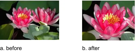
ROCESSING The cropping of images is a step that we introduce to make the flower object in the image clearer and to enhance the segmentation phase by providing the images with less background objects. The following principles have been made to ensure the stability and structure of Oxford flower 102 dataset, each of the following principle will have a flower example to clarify the idea.Cropping single flower.
This cropping principles works on image that contain flower many separated flowers object but one with an accurate and clear view, the wanted image separated using cropping and became the new image main object and placed on the meddle.
a. before b. after
Figure 1: Cropping single flower
Cropping but keep the full bunch.
Some of flowers species the flower itself come in bunches the small flowers combining together to form the whole big flower that sometimes look like bunch of flower, this principle concerning about taking the whole bunch as a shape constraint not only the best looking ones but the whole bunch together.
a. before b. after
Figure 2: Cropping but keep the full bunch
Keeping the same structure (no cropping).
Some of flowers images already came in the form that we want, no obstacles, the flower object are in the meddle and has only one flower.
a b
FIGURE 3: IMAGE WITH NO NEED TO BE CROPPED
5
F
LOWERSS
EGMENTATIONThe Chan-Vese Active Contour Model is a powerful and flexible method as introduced in [13], it is able to segment many types of images considered as difficult to segment in many of classical segmentation approaches such as thresholding or gradient segmentation.
Energy Functional
Chan-Vese main object was introducing a minimization of an energy based segmentation, so they consider the minimization problem as shown in formula (1) and there introduced way for the energy functional minimization Fc1,c2,C defined as shown in formula (2).
) , , (
inf 1 2
, ,2 1 C c c F C c c
Where 0, 0, 1,20 are fixed parameters (should be determined by the user). And as is suggested by [13] they fixed these settings to 0, 12 1.
We have used the following steps to segment the flower object from the images. The active contours work only on gray level images, and we noticed during the training stage that the result that may obtained from the active contour if we apply it over Blue channel of the RBG images is much better than the results that may obtained if we apply it over converted gray level image from our RGB images, because The color difference in gray scale is at its highest, that
dxdy c y x u dxdy c y x u C inside Area C L C c c F C outside C inside
) ( 2 2 0 2 2 )( 0 1
168 better segmentation results over blue layer goes to the
better so we here in this system will work with the Blue channel (channel number 3) of the RGB flower images. Number of maximum iteration which is the number that will end the segmentation process if it have been reached while the contour still moving, smoothness which is the factor that determine the relation between neighbor pixels and size of the mask where the mask is identified as initial contour, are all parameter we obtain during our training stage to be set to 330 as maximum iteration (0.5) as smoothness factor and the mask (outside contour) is equal to the size of image subtracted by 75 pixels from each side.
6
F
EATUREE
XTRACTIONColor, shape and texture are the features that we use as characteristic descriptors, in order to distinguish between our flower object (foreground), and other irrelevant objects (background). Each feature is helpful on specific cases, such that we can distinguish between apple and orange using color, while we can use shape to distinguish between banana and manga. Here in our flower recognition system we will use the invariant moment that described in [14] as our shape feature descriptor, the GLCM as a textures feature extractor which proposed in [15] and the HSV color model as color descriptor that presented by Alvy Ray Smith in 1978 in addition to RGB.
Color features
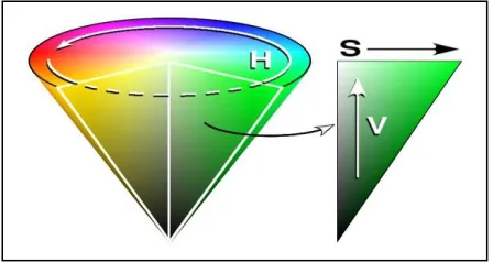
Hue, Saturation and Value together the (HSV) color model which is a model that describes colors in a different way than the RGB (Red, Green, Blue), its preferred approach in this type of works because it is able to eliminate the false data that cased by variation lighting conditions, the hue or (tint) in terms describe the colors shade, saturation which describe the amount of gray level and their brightness or luminance described by the value. HSV color histogram used here in our system as color feature descriptor, the HSV color model using cylinder shape, the Figures (1) describes in cylindrical view the color model of HSV, the following Hue, Saturation and Value describe in detail the meaning of this term.
Figure 4: HSV cylinder (Wikipedia commons)
a) Hue
Hue is the term to describe resemble for the pure color, so red tones and shades have the same hue. The hue values described according to the color wheel position of the corresponding pure color. The hues described as a number between 0° and 360° and as shown in Figure (1) on the top cycle of the cylinder the hues of red begun at (0) where
H=0, yellow at (60) where H=1/6, green at (120) where H=1/3, cyan at (180) where H = 1/2, blue at (240) where H=2/3 and magenta at (300) where H=5/6. For obtaining the Hue value from RGB colored image the formula (3) used.
{ ,( ) (
)-√( ) ( )( )} (3)
a)Saturation
Describe the amount of gray level that describes the whiteness of the color. As the pure colors is fully saturated, so the saturation = 1; the tints of colors have less than 1 saturation; where the white color saturation = 0, and as described on Figure (1) as we go to center of the cylinder the S value goes to zero where is the white color and going to one if we go to the edges of the cycle of the cylinder. For obtaining the Saturation value from RGB colored image the formula (4) used.
( ( )) , ( )- (4)
b)Value
Value or (Brightness) which is a descriptor the works in synchronism with saturation it’s describe the intensity or how bright is the color, the value (V) of a color that also called (lightness), also describes darkness of the color. The value black described as V = 0, and as shown in Figure (1) as we moving from bottom of the cylinder (black) the lightness increasing till we reach the white pure color where V = 1. For obtaining the Brightness value (Value) from RGB colored image the formula (5) used.
( ) (5)
Texture features
Texture is one of the important characteristics used in identifying objects or regions of interest in an image [15], the Gray Level Co-occurrence Matrices GLCM is the most important and one of the earliest texture analyzing approach that have been introduce in 1973 by (Haralick) the using of GLCM P[i, j] starting by specifying the displacement vector (d) which representing as p = (dx, dy) and then calculating the GLCM by counting each pairs of pixels that is separated by (d) as shown in Figure (2).
Figure 5: (a) A 6 x 6 image with two gray levels 0 & 1. (c) The gray-level co-occurrence matrix for (b) the
169 The GLCM is used to provide many statistical features;
here in this paper we will choose the following four statistical features (Contrast, Correlation, Energy, and Homogeneity).
a)Contrast
The contrast statistical feature used to measure the local variations in the gray-level co-occurrence matrix using the formula (6) and returning the contrast of the intensity between the pixels and their neighbors over the entire image.
∑ ( ) (6)
And the range of contrast formula (6) result is calculating based on (7) formula.
Range = [0 (size (GLCM, 1)-1) ^2] (7)
b) Correlation
The correlation statistical feature used to measure the joint probability occurrence using the formula (8) for each specified pixel pairs and returns result that describe how correlated the pixels their neighbors over the entire image.
∑ ( )( ) ( ) (8)
He correlation results come in range = [-1 1]
c) Energy
The statistical Energy feature (known as uniformity or the angular second moment) perform the summation for each squared elements using the formula (9) in the GLCM and returns these sums of the GLCM.
∑ ( ) (9)
The energy results come in range = [0 1]
d) Homogeneity
The statistical Homogeneity feature or known as (inverse Difference Moment) Measures the distribution closeness of the elements in the GLCM using the formula (10) to returns that values of closeness of the distribution of elements in the GLCM to the GLCM diagonal.
∑ ( ) (10)
The homogeneity results come in range = [0 1]
e) Normalizing the probability density of GLCM
The following formula (11) is defined in order to normalize the density of the probability of the Co-occurrence Matrix.
( ) * ( ) ( ) ( ) ( ) + (11)
Where Pδ (i, j) is the probability density; p, q: co-ordinates of the pixel; i, j: gray levels, G is set of pixel pairs and #G is number of G. r is the distance between two pixels i and j.
Shape features
Introduced by [14], he proposed 7th moments features that are invariant to rotation and scaling and used as shape descriptor, the calculation of these seven moments are based on 10 formula they are m00, m10, m01, m11, m20, m02, m21, m12, m30 and m03 and they are as shown below in formula (12, 13, 14, 15, 16, 17, 18, 19, 20 and 21) respectively as they were Introduced by [14].
∑ ∑ , ( ∑ ∑ , (
∑ ∑ , ( ∑ ∑ , (
∑ ∑ , ( ∑ ∑ , (
∑ ∑ , ( ∑ ∑ , (
∑ ∑ , ( )- ∑ ∑ , (
∑ ∑ , ( )- ∑ ∑ , (
∑ ∑ , ( )- ∑ ∑ , (
∑ ∑ , ( )- ∑ ∑ , (
∑ ∑ , ( )- ∑ ∑ , (
∑ ∑ , ( )- ∑ ∑ , (
)-Noting that if calculating of the moments based only according to above formula the moments will not achieve the invariant to the scale or rotate, and in order to make them invariant to rotate the central moment will be used as shown in formula (22).
∫ ∫( ̅) ( ̅) ( )
Where
̅
̅
And the point ( ̅ ̅) are the centroid f(x, y) image. And to make them invariant to scale the normalization used to normalize the central moments shown in formula (23).
(23)
The seven invariant to scale and translation moment are calculated as following.
- First moment
(24)
- Second moment
( ) (25)
- Third moment
( ) ( ) (26)
- Forth moment
( ) ( ) (27)
- Fifth moment
(12) (13) (14) (15) (16) (17) (18) (19) (20) (21)
170
( )( ),( ) ( ) -
( )( ), ( ) ( )
-- Sixth moment
- ( ),( ) ( ) -
( )( )
- Seventh moment
- ( )( ),(
) ( ) - (
)( ), ( )
( )
-7
F
LOWERC
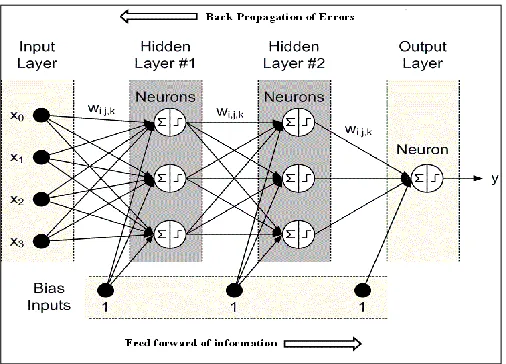
LASSIFICATIONAs a classification of supervised learning, the back-propagation network Figure (3) is a good example of it, Back-propagation is a popular form of training multi-layer neural networks, and is a classic topic in neural network courses. It has the advantages of accuracy and versatility. Sample inputs is repeatedly presented to the input layer, to compare the desired activation of the output layer for them, with the actual activation of the output layer, adjustments are made on weights in learning network process until a set of weights that produce the correct output for every sample input is found. The advantages of back-propagation are its simple, local nature. In the back propagation algorithm, each hidden unit passes and receives information only to and from units that share a connection. Hence it can be implemented efficiently on a parallel architecture computer [16].
Figure 6: Back Propagation NN model
There are many activation functions that used in associated with back-propagation such as step, sign and sigmoid function, and as shown in Figure (4). In this proposed study we used the sigmoid activation function because its produce only positive number and it can be used with gradient descent based training because it has a derivative.
( ) { ( )
{ ( )
Figure 7: Activation Functions
The algorithm for back-propagation network may consist of four steps:
1) Feed-forward computation
2) Back propagation to the output layer 3) Back propagation to the hidden layer 4) Weight updates
And when the value of the error function has become small the algorithm is stopped. The back-propagation can be summarized as follows:
1) Back-propagation is a good example of supervised learning.
2) In training process inputs and their corresponding outputs are supplied to the network repeatedly. 3) Error signals is calculated by the network that used
to adjust weights.
4) When applying many passes, a low error is settled by the network on the training data.
Then it’s tested on new test data, to measure that if it can be generalized.
8
R
ESULTSHere in this proposed study we simulate our methodology using MATLAB 2013 and HP core i7, 8 G.B RAM, so after we obtain our features matrices from the segmented images of 102 Oxford data set using chan-vese active contour for segmentation and HSV, GLCM and IM for color, texture and shape respectively we used MATLAB Neural Network tools for classifying our flowers based on obtained features and as following.
f) Segmentation results
The images have been segmented using chan-vese active contour using MATLAB, the segmented image results have been categorized into 3 category perfect, acceptable and non-desire according to the formula (31) and as results shown in table (1).
∁ = (A, B, C)/T (31)
Where A, B and C are the three category, and T is the total number of data.
(28)
(29)
171
Table 1: segmentation results matrices
Category A, perfect B, Acceptable C, Not desire
Ratio 70.89% 21.04% 8.07%
g) Feature extraction results
The features matrices obtained from segmented image collected in 7 matrices in order to make the classification process based on these 7 matrices; one for classifying according to the HSV, GLCM and IM separately and then combining 2 of these matrices together as color and shape, color and texture, and texture and shape, and the final matrices for all of color, shape and texture together.
h) Neural network classification results
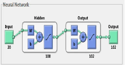
As we described before the classification process will be implemented over 7 times in order to obtain the results of classification for all of 7 obtained features matrices, the Figure (5) shows the MATLAB neural network diagram that we use in our simulation.
Figure 8: Neural Network MATLAB diagram
There are 2 sets of numbers that are required to run the ANN classification tool, the first one is the input data which is the features matrices that we already obtained and the second one is the target data which is a data that identified each flower and shows which class that each flower belong to. The accuracy that achieved using the 7 features matrices are shown in table (2), between the 700 and 800 iteration training the maximum accurate results occur using 1 hidden layer that contain 100 neurons. Table (2) showing the classification process accuracy results using the ANN for the 7th obtained features matrices.
Table 2: the training results using 7 features matrices summary
Features in Use
Accuracy achieved Classified flowers
rate
Error Occurred Misclassified flower
rate
color :5.86% 9>.14%
texture 99.36% ::.64%
shape 8>.15% ;5.85%
Color and texture <7.42% 7<.58%
Color and shape ;8.58% 8;.42%
Shape and texture ;6.80% 8=.20%
Color, shape and
texture 81.19% 6=.81%
As a Comparison with related work the website of Oxford 102 dataset contains a comparison between 5 studies that works on the 102 dataset, showing their results as an accuracy results. The following table (3) shows the methodology comparison between these five related work and our methodology.
Table 3: comparing table for 102 oxford dataset related studies
The table (3) contain simple comparison between (Oxford 102) 5 related studies that mentioned on their website, the used features and segmentation phase have been marked with (√), while the unused feature or segmentation phase have been marked with (-), and in classifier field we mentioned the used classification approach. Another detailed comparison has been carried out between our recognition system and [10]. And as shown in table (4), the comparison has been done based on the data that have been used on their paper and was taken from their publication website (Bi-CoS website) [20].
Table 4: Detailed comparing table between our methodology and [10]
Study Our Methodology Chai et al. (2011)
segmentations CVAC BiCoS-MT
Features extraction
Color CM BoW
Texture GLCM -
Shape IM SIFT descriptor
classifier ANN SVM
ACU% 81.19% 80.00%
In [10] they have used 2040 images for their work, they have selected 20 images for each species to implement their work. They used their new segmentation approach Bi-CoS for the segmentation phase without any enhancement techniques, while we used the cropping as enhancement and CVAC for segmentation. For the feature extraction phase they used only. Color and shape descriptor, BoW and SIFT respectively, while we used color, shape, and texture. We have used color moment, GLCM and IM respectively for the selected features. The achieved results show that we pass them with 1.19% in accuracy. we achieved 81.19% after we categorized our obtained features matrices with respect to segmentation quality, while they achieved 80% accuracy on the same selected flowers images of the Oxford 102 dataset.
172
9
C
ONCLUSIONSA
NDR
ECOMMENDATIONSIn this proposed study we created a CAFR system based on image processing techniques and ANN; the image processing techniques used for steps of enhancements, features extraction and segmentation. The enhancements have been done by cropping the dataset images to fit the CVAC, where the automated CVAC used for segmenting the flower object from the images backgrounds, the phase of features extraction was done using color moments, GLCM and IM for color, textures and shape respectively. The comparison that have been carried out on this proposed paper, was based on partial data that include all flowers species with 20 images for each, this data has been selected by [10], they have achieved 80% of accuracy, while we achieved 81.19% on the same selected partial data based on assumptions. And from this point we can consider implementing our system on the whole data as one of the future works. The work have been done in this paper is considered as one step in a long science journey, many of modification and future works are available; like enhancing the output of segmentation process by modifying parameters of active contour model or by using another segmentation approach, there are many color, texture and shape descriptor may be used as replacements of our used approach or same descriptor in deferent approaches, the ANN is wide area of research, as the number of neurons inside layers considers as optimization problem and a lot of work could be done only by working on the ANN parameters and features.
References
[1] Zanchettin, C., Bezerra, B. L. D., & Azevedo, W. W. (2012, June). A KNN-SVM hybrid model for cursive handwriting recognition. In Neural Networks (IJCNN), The 2012 International Joint Conference on (pp. 1-8). IEEE.
[2] Conti, V., Militello, C., Vitabile, S., & Sorbello, F. (2010). Complex,―Fingerprint Recognition‖ Intelligent and Software Intensive Systems (CISIS). In 2010 International Conference (pp. 368-375).
[3] Guocai Liu; Weili Yang; Suyu Zhu; Qiu Huang; Min Liu; Haiyan Wu; Zetian Hu; Zaijie Huang; Yuan Yuan; Ke Liu; Wenlin Huang; Bin Liu; Jinguang Liu; Xuping Zhao; Mao Nie; Bingqiang Hu; Jiutang Zhang; Yi Mo; Biao Zeng; Xiang Peng; Jumei Zhou, "PET/CT image textures for the recognition of tumors and organs at risk for radiotherapy treatment planning," in Nuclear Science Symposium and Medical Imaging Conference (NSS/MIC), 2013 IEEE , vol., no., pp.1-3
[4] Siraj F, Ekhsan H M and Zulkifli A N (2014), Flower image classification modeling using neural network. In Computer, Control, Informatics and Its Applications (IC3INA), International Conference on (pp. 81-86). IEEE.
[5] Tai-Shan Yan, Yong-Qing Tao and Du-wu Cui(2007), Research on handwritten numeral recognition method based on improved genetic algorithm and neural network. Wavelet Analysis
and Pattern Recognition. ICWAPR '07. International Conference on, vol.3, no., pp.1271,1276.
[6] Hsu T H, Lee C H and Chen L H (2011), An interactive flower image recognition system. Multimedia Tools and Applications, 53(1), 53-73.
[7] Saitoh T, Aoki K and Kaneko T (2004), Automatic recognition of blooming flowers. In Pattern Recognition, ICPR. Proceedings of the 17th International Conference on (Vol. 1, pp. 27-30). IEEE.
[8] Phyu K H, Kutics A and Nakagawa A (2012), Self-adaptive Feature Extraction Scheme for Mobile Image Retrieval of Flowers. In Signal Image Technology and Internet Based Systems (SITIS), Eighth International Conference on (pp. 366-373). IEEE.
[9] Nilsback M E, and Zisserman A (2007), Delving into the Whorl of Flower Segmentation. In BMVC (pp. 1-10).
[10] Chai Y, Lempitsky V and Zisserman A (2011), Bicos: A bi-level co-segmentation method for image classification. Master thesis
[11] Nilsback M E and Zisserman A (2009), An automatic visual flora: segmentation and classification of flower images (Doctoral dissertation, Oxford University).
[12] Tiay T, Benyaphaichit P, and Riyamongkol P (2014), Flower Recognition System Based on Image Processing. In Student Project Conference (ICT-ISPC), Third ICT International (pp. 99-102). IEEE.
[13] T Chan and L Vese(2001), Active contours without edges. in IEEE transactions on image processing 10(2), pp. 266-277.
[14] Hu M K (1962), Visual pattern recognition by moment invariants. Information Theory, IRE Transactions on, 8(2), 179-187.
[15] Haralick Robert M, Karthikeyan Shanmugam and Its' Hak Dinstein(1973), Textural features for image classification. Systems, Man and Cybernetics, IEEE Transactions on 6 (1973): 610-621.
[16] Trevor J.. Hastie, Tibshirani, R. J., & Friedman, J. H. (2009). The elements of statistical learning: data mining, inference, and prediction. Springer.
173 [18] Kanan C and Cottrell G (2010), Robust
classification of objects, faces, and flowers using natural image statistics. In Computer Vision and Pattern Recognition (CVPR), IEEE Conference on (pp. 2472-2479).
[19] Ito S and Kubota S (2010), Object classification using heterogeneous co-occurrence features. In Computer Vision–ECCV 2010 (pp. 701-714). Springer Berlin Heidelberg.