Accuracy, robustness and scalability of dimensionality reduction methods for single cell RNA seq analysis

R E S E A R C H

Open Access

Accuracy, robustness and scalability of

dimensionality reduction methods for

single-cell RNA-seq analysis

Shiquan Sun

, Jiaqiang Zhu

, Ying Ma

and Xiang Zhou

Abstract

Background:Dimensionality reduction is an indispensable analytic component for many areas of single-cell RNA sequencing (scRNA-seq) data analysis. Proper dimensionality reduction can allow for effective noise removal and facilitate many downstream analyses that include cell clustering and lineage reconstruction. Unfortunately, despite the critical importance of dimensionality reduction in scRNA-seq analysis and the vast number of dimensionality reduction methods developed for scRNA-seq studies, few comprehensive comparison studies have been performed to evaluate the effectiveness of different dimensionality reduction methods in scRNA-seq.

Results:We aim to fill this critical knowledge gap by providing a comparative evaluation of a variety of commonly used dimensionality reduction methods for scRNA-seq studies. Specifically, we compare 18 different dimensionality reduction methods on 30 publicly available scRNA-seq datasets that cover a range of sequencing techniques and sample sizes. We evaluate the performance of different dimensionality reduction methods for neighborhood preserving in terms of their ability to recover features of the original expression matrix, and for cell clustering and lineage reconstruction in terms of their accuracy and robustness. We also evaluate the computational scalability of different dimensionality reduction methods by recording their computational cost.

Conclusions:Based on the comprehensive evaluation results, we provide important guidelines for choosing dimensionality reduction methods for scRNA-seq data analysis. We also provide all analysis scripts used in the present study atwww.xzlab.org/reproduce.html.

Introduction

Single-cell RNA sequencing (scRNA-seq) is a rapidly grow-ing and widely applygrow-ing technology [1–3]. By measuring gene expression at a single-cell level, scRNA-seq provides an unprecedented opportunity to investigate the cellular heterogeneity of complex tissues [4–8]. However, despite the popularity of scRNA-seq, analyzing scRNA-seq data re-mains a challenging task. Specifically, due to the low cap-ture efficiency and low sequencing depth per cell in scRNA-seq data, gene expression measurements obtained from scRNA-seq are noisy: collected scRNA-seq gene mea-surements are often in the form of low expression counts, and in studies not based on unique molecular identifiers,

are also paired with an excessive number of zeros known as

dropouts [9]. Subsequently, dimensionality reduction

methods that transform the original high-dimensional noisy expression matrix into a low-dimensional subspace with enriched signals become an important data processing step for scRNA-seq analysis [10]. Proper dimensionality reduc-tion can allow for effective noise removal, facilitate data visualization, and enable efficient and effective downstream analysis of scRNA-seq [11].

Dimensionality reduction is indispensable for many types of scRNA-seq analysis. Because of the importance of dimensionality reduction in scRNA-seq analysis, many dimensionality reduction methods have been developed and are routinely used in scRNA-seq software tools that include, but not limited to, cell clustering tools [12,13] and lineage reconstruction tools [14]. Indeed, most com-monly used scRNA-seq clustering methods rely on dimensionality reduction as the first analytic step [15].

© The Author(s). 2019Open AccessThis article is distributed under the terms of the Creative Commons Attribution 4.0 International License (http://creativecommons.org/licenses/by/4.0/), which permits unrestricted use, distribution, and reproduction in any medium, provided you give appropriate credit to the original author(s) and the source, provide a link to the Creative Commons license, and indicate if changes were made. The Creative Commons Public Domain Dedication waiver (http://creativecommons.org/publicdomain/zero/1.0/) applies to the data made available in this article, unless otherwise stated. * Correspondence:[email protected]

2

Department of Biostatistics, University of Michigan, Ann Arbor, MI 48109, USA

3_{Center for Statistical Genetics, University of Michigan, Ann Arbor, MI 48109,} USA

For example, Seurat applies clustering algorithms dir-ectly on a low-dimensional space inferred from principal

component analysis (PCA) [16]. CIDR improves

cluster-ing by improvcluster-ing PCA through imputation [17]. SC3

combines different ways of PCA for consensus clustering [18]. Besides PCA, other dimensionality reduction tech-niques are also commonly used for cell clustering. For example, nonnegative matrix factorization (NMF) is used in SOUP [19]. Partial least squares is used in scPLS [20]. Diffusion map is used in destiny [21]. Multidimensional scaling (MDS) is used in ascend [22]. Variational infer-ence autoencoder is used in scVI [23]. In addition to cell clustering, most cell lineage reconstruction and develop-mental trajectory inference algorithms also rely on

di-mensionality reduction [14]. For example, TSCAN

builds cell lineages using minimum spanning tree based

on a low-dimensional PCA space [24]. Waterfall

per-formsk-means clustering in the PCA space to eventually produce linear trajectories [25]. SLICER uses locally lin-ear embedding (LLE) to project the set of cells into a lower-dimension space for reconstructing complex cellu-lar trajectories [26]. Monocle employs either independ-ent componindepend-ents analysis (ICA) or uniform manifold approximation and projection (UMAP) for dimensional-ity reduction before building the trajectory [27, 28]. Wishbone combines PCA and diffusion maps to allow for bifurcation trajectories [29].

Besides the generic dimensionality reduction methods mentioned in the above paragraph, many dimensionality reduction methods have also been developed recently that are specifically targeted for modeling scRNA-seq data. These scRNA-seq-specific dimensionality reduction methods can account for either the count nature of scRNA-seq data and/or the dropout events commonly encountered in scRNA-seq studies. For example, ZIFA relies on a zero-inflation normal model to model

drop-out events [30]. pCMF models both dropout events and

the mean-variance dependence resulting from the count

nature of scRNA-seq data [31]. ZINB-WaVE

incorpo-rates additional gene-level and sample-level covariates for more accurate dimensionality reduction [32]. Finally, several deep learning-based dimensionality reduction methods have recently been developed to enable scalable and effective computation in large-scale scRNA-seq data, including data that are collected by 10X Genomics

tech-niques [33] and/or from large consortium studies such

as Human Cell Atlas (HCA) [34, 35]. Common deep

learning-based dimensionality reduction methods for

scRNA-seq include Dhaka [36], scScope [37], VASC

[38], scvis [39], and DCA [40], to name a few.

With all these different dimensionality reduction methods for scRNA-seq data analysis, one naturally wonders which dimensionality reduction method one would prefer for different types of scRNA-seq analysis.

Unfortunately, despite the popularity of scRNA-seq technique, the critical importance of dimensionality re-duction in scRNA-seq analysis, and the vast number of dimensionality reduction methods developed for scRNA-seq studies, few comprehensive comparison studies have been performed to evaluate the effectiveness of different dimensionality reduction methods for practical applica-tions. Here, we aim to fill this critical knowledge gap by providing a comprehensive comparative evaluation of a variety of commonly used dimensionality reduction methods for scRNA-seq studies. Specifically, we com-pared 18 different dimensionality reduction methods on 30 publicly available scRNA-seq data sets that cover a range of sequencing techniques and sample sizes [12,14,

41]. We evaluated the performance of different

dimen-sionality reduction methods for neighborhood preserving in terms of their ability to recover features of the original expression matrix, and for cell clustering and lineage re-construction in terms of their accuracy and robustness using different metrics. We also evaluated the computa-tional scalability of different dimensionality reduction methods by recording their computational time. To-gether, we hope our results can serve as an important guideline for practitioners to choose dimensionality re-duction methods in the field of scRNA-seq analysis.

Results

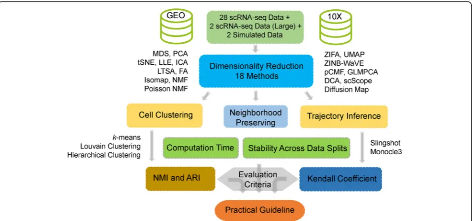
We evaluated the performance of 18 dimensionality re-duction methods (Table 1; Additional file 1: Figure S1) on 30 publicly available scRNA-seq data sets (Add-itional file1: Table S1-S2) and 2 simulated data sets.

De-tails of these data sets are provided in “Methods and

Materials.”Briefly, these data sets cover a wide variety of

sequencing techniques that include Smart-Seq2 [1] (8

different dimensionality reduction methods and recorded their computation time. An overview of the comparison workflow is shown in Fig.1. Because common tSNE software can only extract a small number low-dimensional compo-nents [48,58, 59], we only included tSNE results based on two low-dimensional components extracted from the re-cently developed fastFIt-SNE R package [48] in all figures. All data and analysis scripts for reproducing the results in the paper are available at www.xzlab.org/reproduce.htmlor

https://github.com/xzhoulab/DRComparison.

Performance of dimensionality reduction methods for neighborhood preserving

We first evaluated the performance of different dimen-sionality reduction methods in terms of preserving the original features of the gene expression matrix. To do

so, we applied different dimensionality reduction

methods to each of 30 scRNA-seq data sets (28 real data and 2 simulated data; excluding the two large-scale data due to computing concerns) and evaluated the perform-ance of these dimensionality reduction methods based on neighborhood preserving. Neighborhood preserving measures how the local neighborhood structure in the

reduced dimensional space resembles that in the original

space by computing a Jaccard index [60] (details in

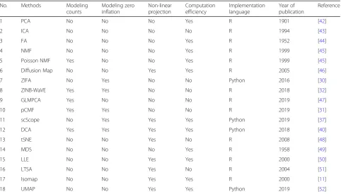
“Methods and Materials”). In the analysis, for each di-mensionality reduction method and each scRNA-seq data set, we applied the dimensionality reduction method to extract a fixed number of low-dimensional components (e.g., these are the principal components in the case of PCA). We varied the number of low-dimensional components to examine their influence on local neighborhood preserving. Specifically, for each of 16 cell clustering data sets, we varied the number of low-dimensional components to be either 2, 6, 14, or 20 when the data contains less than or equal to 300 cells, and we varied the number of low-dimensional compo-nents to be either 0.5%, 1%, 2%, or 3% of the total num-ber of cells when the data contains more than 300 cells. For each of the 14 trajectory inference data sets, we varied the number of low-dimensional components to be either 2, 6, 14, or 20 regardless of the number of cells. Finally, we also varied the number of neighborhood cells used in the Jaccard index to be either 10, 20, or 30. The evaluation re-sults based on the Jaccard index of neighborhood preserv-ing are summarized in Additional file1: Figure S2-S14. Table 1List of compared dimensionality reduction methods. We list standard modeling properties for each of compared dimensionality reduction methods

No. Methods Modeling

counts

Modeling zero inflation

Non-linear projection

Computation efficiency

Implementation language

Year of publication

Reference

1 PCA No No No Yes R 1901 [42]

2 ICA No No No No R 1994 [43]

3 FA No No No Yes R 1952 [44]

4 NMF No No No Yes R 1999 [45]

5 Poisson NMF Yes No No Yes R 1999 [45]

6 Diffusion Map No No Yes Yes R 2005 [46]

7 ZIFA No Yes No No Python 2016 [30]

8 ZINB-WaVE Yes Yes No No R 2018 [32]

9 GLMPCA Yes No No No R 2019 [47]

10 pCMF Yes Yes No No R 2019 [31]

11 scScope No Yes Yes Yes Python 2019 [37]

12 DCA Yes Yes Yes Yes Python 2018 [40]

13 tSNE No No Yes No R 2008 [48]

14 MDS No No No Yes R 1958 [49]

15 LLE No No Yes Yes R 2000 [50]

16 LTSA No No Yes No R 2004 [51]

17 Isomap No No Yes Yes R 2000 [11]

18 UMAP No No Yes Yes Python 2019 [52]

These properties include whether it models count data (3rd column), whether it accounts for zero inflation (4th column), whether it is a linear dimensionality reduction method (5th column), its computation efficiency (6th column), implementation language (7th column), year of publication (8th column), and reference (9th column).FA

factor analysis,PCAprincipal component analysis,ICAindependent component analysis,NMFnonnegative matrix factorization,Poisson NMFKullback-Leibler divergence-based NMF,ZIFAzero-inflated factor analysis,ZINB-WaVEzero-inflated negative binomial-based wanted variation extraction,pCMFprobabilistic count matrix

In the cell clustering data sets, we found that pCMF achieves the best performance of neighborhood preserving across all data sets and across all included low-dimensional components (Additional file1: Figure S2-S7). For example, with 30 neighborhood cells and 0.5% of low-dimensional components, pCMF achieves a Jaccard index of 0.25. Its performance is followed by Poisson NMF (0.16), ZINB-WaVE (0.16), Diffusion Map (0.16), MDS (0.15), and tSNE (0.14). While the remaining two methods, scScope (0.1) and LTSA (0.06), do not fare well. Increasing number of neighborhood cells increases the ab-solute value of Jaccard index but does not influence the relative performance of dimensionality reduction methods (Additional file1: Figure S7). In addition, the relative per-formance of most dimensionality reduction methods re-mains largely similarly whether we focus on data sets with unique molecular identifiers (UMI) or data sets without UMI (Additional file1: Figure S8). However, we do notice two exceptions: the performance of pCMF decreases with increasing number of low-dimensional components in UMI data but increases in non-UMI data; the ance of scScope is higher in UMI data than its perform-ance in non-UMI data. In the trajectory inference data sets, pCMF again achieves the best performance of

neighborhood preserving across all data sets and across all included low-dimensional components (Additional file1: Figure S9-S14). Its performance is followed closely by scScope and Poisson NMF. For example, with 30 neigh-borhood cells and 20 low-dimensional components, the Jaccard index of pCMF, Poisson NMF, and scScope across all data sets are 0.3, 0.28, and 0.26, respectively. Their per-formance is followed by ZINB-WaVE (0.19), FA (0.18), ZIFA (0.18), GLMPCA (0.18), and MDS (0.18). In con-trast, LTSA also does not fare well across all included

low-dimensional components (Additional file 1: Figure

S14). Again, increasing number of neighborhood cells in-creases the absolute value of Jaccard index but does not influence the relative performance among dimensionality reduction methods (Additional file1: Figure S9-S14).

We note that the measurement we used in this subsec-tion, neighborhood preserving, is purely for measuring dimensionality reduction performance in terms of pre-serving the original gene expression matrix and may not be relevant for single-cell analytic tasks that are the main focus of the present study: a dimensionality reduction method that preserves the original gene expression matrix may not be effective in extracting useful bio-logical information from the expression matrix that is

essential for key downstream single-cell applications. Preserving the original gene expression matrix is rarely the sole purpose of dimensionality reduction methods for single-cell applications: indeed, the original gene expression matrix (which is the best-preserved matrix of itself) is rarely, if ever, used directly in any down-stream single-cell applications including clustering and lineage inference, even though it is computation-ally easy to do so. Therefore, we will focus our main comparison in two important downstream single-cell applications listed below.

Performance of dimensionality reduction methods for cell clustering

As our main comparison, we first evaluated the perform-ance of different dimensionality reduction methods for cell clustering applications. To do so, we obtained 14 publicly available scRNA-seq data sets and simulated

two additional scRNA-seq data sets using the Splatter

package (Additional file1: Table S1). Each of the 14 real scRNA-seq data sets contains known cell clustering in-formation while each of the 2 simulated data sets con-tains 4 or 8 known cell types. For each dimensionality reduction method and each data set, we applied dimen-sionality reduction to extract a fixed number of low-dimensional components (e.g., these are the principal components in the case of PCA). We again varied the number of low-dimensional components as in the previ-ous section to examine their influence on cell clustering analysis. We then applied either the hierarchical

cluster-ing method, the k-means clustering method, or Louvain

clustering method [61] to obtain the inferred cluster la-bels. We used both normalized mutual information (NMI) and adjusted rand index (ARI) values for compar-ing the true cell labels and inferred cell labels obtained by clustering methods based on the low-dimensional components.

Cell clustering with different clustering methods

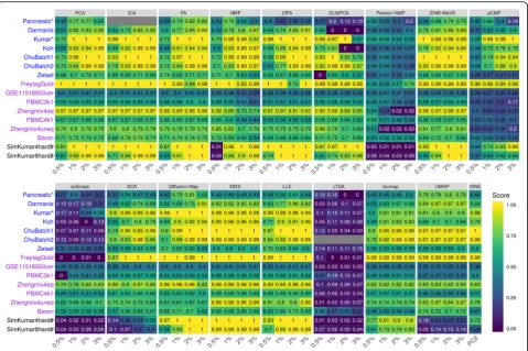
The evaluation results on dimensionality reduction

methods based on clustering analysis using thek-means

clustering algorithm are summarized in Fig.2 (for NMI

criterion) and Additional file 1: Figure S15 (for ARI cri-terion). Because the results based on either of the two criteria are similar, we will mainly explain the results

based on the NMI criteria in Fig. 2. For easy

visualization, we also display the results averaged across data sets in Additional file1: Figure S16. A few patterns are noticeable. First, as one would expect, clustering ac-curacy depends on the number of low-dimensional com-ponents that are used for clustering. Specifically, accuracy is relatively low when the number of included low-dimensional components is very small (e.g., 2 or 0.5%) and generally increases with the number of

included components. In addition, accuracy usually satu-rates once a sufficient number of components is in-cluded, though the saturation number of components can vary across data sets and across methods. For ex-ample, the average NMI across all data sets and across all methods are 0.61, 0.66, 0.67, and 0.67 for increasingly large number of components, respectively. Second, when conditional on using a low number of components, scRNA-seq-specific dimensionality reduction method

ZINB-WaVE and generic dimensionality reduction

methods ICA and MDS often outperform the other methods. For example, with the lowest number of com-ponents, the average NMI across all data sets for MDS, ICA, and ZINB-WaVE are 0.82, 0.77 and 0.76, respect-ively (Additional file 1: Figure S16A). The performance of MDS, ICA, and ZINB-WaVE is followed by LLE (0.75), Diffusion Map (0.71), ZIFA (0.69), PCA (0.68), FA (0.68), tSNE (0.68), NMF (0.59), and DCA (0.57). While the remaining four methods, Poisson NMF (0.42), pCMF (0.41), scScope (0.26), and LTSA (0.12), do not fare well with a low number of components. Third, with increasing number of low-dimensional components, gen-eric methods such as FA, ICA, MDS, and PCA are often comparable with scRNA-seq-specific methods such as ZINB-WaVE. For example, with the highest number of low-dimensional components, the average NMI across all data sets for FA, ICA, PCA, ZINB-WaVE, LLE, and MDS are 0.85, 0.84, 0.83, 0.83, 0.82, and 0.82, respect-ively. Their performance is followed by ZIFA (0.79), NMF (0.73), and DCA (0.69). The same four methods, pCMF (0.55), Poisson NMF (0.31), scScope (0.31), and LTSA (0.06) again do not fare well with a large number

of low-dimensional components (Additional file 1:

Fig-ure S16A). The comparable results of generic dimen-sionality reduction methods with scRNA-seq-specific dimensionality reduction methods with a high number of low-dimensional components are also consistent some of the previous observations; for example, the ori-ginal ZINB-WaVE paper observed that PCA can gener-ally yield comparable results with scRNA-seq-specific dimensionality reduction methods in real data [32].

Besides thek-means clustering algorithm, we also used the hierarchical clustering algorithm to evaluate the per-formance of different dimensionality reduction methods (Additional file 1: Figure S17-S19). In this comparison, we had to exclude one dimensionality reduction method, scScope, as hierarchical clustering does not work on the extracted low-dimensional components from scScope. Consistent with thek-means clustering results, we found that the clustering accuracy measured by hierarchical clustering is relatively low when the number of low-dimensional components is very small (e.g., 2 or 0.5%), but generally increases with the number of included

clustering results, we found that generic dimensionality reduction methods often yield results comparable to or better than scRNA-seq-specific dimensionality reduction methods (Additional file 1: Figure S17-S19). In particu-lar, with a low number of low-dimensional components,

MDS achieves the best performance (Additional file 1:

Figure S19). With a moderate or high number of low-di-mensional components, two generic dilow-di-mensionality reduction methods, FA and NMF, often outperform

various other dimensionality reduction methods

across a range of settings. For example, when the number of low-dimensional components is moderate (6 or 1%), both FA and NMF achieve an average

NMI value of 0.80 across data sets (Additional file 1:

Figure S19A). In this case, their performance is followed by PCA (0.72), Poisson NMF (0.71), ZINB-WaVE (0.71), Diffusion Map (0.70), LLE (0.70), ICA (0.69), ZIFA (0.68), pCMF (0.65), and DCA (0.63). tSNE (0.31) does not fare well, either because it only extracts two-dimensional components or because it does not pair well with hierarchical clustering. We note, however, that the clustering results obtained by hierarchical clustering are often slightly worse than

that obtained by k-means clustering across settings

(e.g., Additional file 1: Figure S16 vs Additional file1: Figure S19), consistent with the fact that many

scRNA-seq clustering methods use k-means as a key

ingredient [18, 25].

Finally, besides thek-means and hierarchical clustering methods, we also performed clustering analysis based on a community detection algorithm Louvain clustering method [61]. Unlike thek-means and hierarchical clus-tering methods, Louvain method does not require a pre-defined number of clusters and can infer the number of clusters in an automatic fashion. Following software recommendation [28, 61], we set the k-nearest neighbor parameter in Louvain method to be 50 for graph building in the analysis. We measured dimensionality reduction performance again by either average NMI (Additional file1: Figure S20) or ARI (Additional file1: Figure S21). Consist-ent with thek-means clustering results, we found that the clustering accuracy measured by Louvain method is rela-tively low when the number of low-dimensional compo-nents is very small (e.g., 2 or 0.5%), but generally increases with the number of included components. With a low number of low-dimensional components, ZINB-WaVE (0.72) achieves the best performance (Additional file 1: Figure S20-S22). With a moderate or high number of low-dimensional components, two generic low-dimensionality reduction methods, FA and MDS, often outperform vari-ous other dimensionality reduction methods across a range of settings (Additional file1: Figure S20-S22). For example, when the number of low-dimensional components is high (6 or 1%), FA achieves an average NMI value of 0.77 across data sets (Additional file1: Figure S22A). In this case, its performance is followed by NMF (0.76), MDS (0.75), GLMPCA (0.74), LLE (0.74), PCA (0.73), ICA (0.73), ZIFA (0.72), and ZINB-WaVE (0.72). Again consistent with the k-means clustering results, scScope (0.32) and LTSA (0.21) do not fare well. We also note that the clustering results obtained by Louvain method are often slightly worse than that obtained by k-means clustering and slightly better than that obtained by hierarchical clustering across settings (e.g., Additional file 1: Figure S16 vs Additional file 1: Figure S19 vs Additional file1: Figure S22).

Normalization does not influence the performance of dimensionality reduction methods

While some dimensionality reduction methods (e.g., Poisson NMF, ZINB-WaVE, pCMF, and DCA) directly model count data, many dimensionality reduction methods (e.g., PCA, ICA, FA, NMF, MDS, LLE, LTSA, Isomap, Diffusion Map, UMAP, and tSNE) require nor-malized data. The performance of dimensionality reduc-tion methods that use normalized data may depend on how data are normalized. Therefore, we investigated how different normalization approaches impact on the performance of the aforementioned dimensionality re-duction methods that use normalized data. We exam-ined two alternative data transformation approaches, log2 CPM (count per million; 11 dimensionality reduc-tion methods), and z-score (10 dimensionality reduction

methods), in addition to the log2 count we used in the previous results (transformation details are provided in “Methods and Materials”). The evaluation results are

summarized in Additional file 1: Figure S23-S30 and are generally insensitive to the transformation approach

deployed. For example, with the k-means clustering

algorithm, when the number of low-dimensional com-ponents is small (1%), PCA achieves an NMI value of 0.82, 0.82, and 0.81, for log2 count transformation,

log2 CPM transformation, and z-score transformation,

respectively (Additional file 1: Figure S16A, S26A, and

S30A). Similar results hold for the hierarchical

clustering algorithm (Additional file 1: Figure S16B,

S26B, and S30B) and Louvain clustering method

(Additional file 1: Figure S16C, S26C, and S30C).

Therefore, different data transformation approaches do not appear to substantially influence the perform-ance of dimensionality reduction methods.

Performance of dimensionality reduction methods in UMI vs non-UMI-based data sets

methods are 0.83, 0.81, 0.80, 0.78, and 0.77, respectively. With increasing number of low-dimensional components, four additional dimensionality reduction methods, PCA, ICA, FA, and ZINB-WaVE, also start to catch up. How-ever, a similar set of dimensionality reduction methods, in-cluding GLMPCA, Poisson NMF, scScope, LTSA, and occasionally pCMF, also do not perform well in these non-UMI data sets.

Visualization of clustering results

We visualized the cell clustering results in two example data sets: the Kumar data which is non-UMI based and the PBMC3k data which is UMI based. The Kumar data consists of mouse embryonic stem cells cultured in three different media while the PBMC3k data consists of 11 blood cell types (data details in the Additional file 1). Here, we extracted 20 low-dimensional components in the Kumar data and 32 low low-dimensional compo-nents in the PBMC3k data with different dimensionality reduction methods. We then performed tSNE analysis on these low-dimensional components to extract the two tSNE components for visualization (Additional file1: Figure S32-S33). Importantly, we found that the tSNE visualization results are not always consistent with clus-tering performance for different dimensionality reduc-tion methods. For example, in the Kumar data, the low-dimensional space constructed by FA, pCMF, and MDS often yield clear clustering visualization with distinguish clusters (Additional file 1: Figure S32), consistent with their good performance in clustering (Fig. 2). However, the low-dimensional space constructed by PCA, ICA, and ZIFA often do not yield clear clustering visualization

(Additional file 1: Figure S32), even though these

methods all achieve high cell clustering performance (Fig.2). Similarly, in the PBMC3k data set, FA and MDS perform well in clustering visualization (Additional file1: Figure S33), which is consistent with their good

per-formance in clustering analysis (Fig. 2). However, PCA

and ICA do not fare well in clustering visualization (Additional file1: Figure S33), even though both of them

achieve high clustering performance (Fig. 2). The

in-consistency between cluster visualization and cluster-ing performance highlights the difference in the analytic goal of these two analyses: cluster visualization emphasizes on extracting as much information as pos-sible using only the top two-dimensional components, while clustering analysis often requires a much larger number of low-dimensional components to achieve accurate performance. Subsequently, dimensionality reduction methods for data visualization may not fare well for cell clustering, and dimensionality reduction methods for cell clustering may not fare well for data visualization [20].

Rare cell type identification

So far, we have focused on clustering performance in terms of assigning all cells to cell types without distinguishing whether the cells belong to a rare population or a non-rare population. Identifying rare cell populations can be of sig-nificant interest in certain applications and performance of rare cell type identification may not always be in line with general clustering performance [62,63]. Here, we examine the effectiveness of different dimensionality reduction methods in facilitating the detection of rare cell popula-tions. To do so, we focused on the PBMC3k data from 10X

Genomics [33]. The PBMC3k data were measured on 3205

cells with 11 cell types. We considered CD34+ cell type (17 cells) as the rare cell population. We paired the rare cell population with either CD19+ B cells (406 cells) or CD4+/ CD25 T Reg cells (198) cells to construct two data sets with different rare cell proportions. We named these two data sets PBMC3k1Rare1 and PBMC3k1Rare2, respectively. We then applied different dimensionality reduction methods to each data and usedF-measure to measure the performance of rare cell type detection following [64, 65] (details in “Methods and Materials”). The results are summarized in

Additional file1: Figure S34-S35.

Overall, we found that Isomap achieves the best per-formance for rare cell type detection across a range of low-dimensional components in both data sets with dif-ferent rare cell type proportions. As expected, the ability to detect rare cell population increases with increasing rare cell proportions. In the PBMC3k1Rare1 data, theF -measure by Isomap with four different number of low-dimensional components (0.5%, 1%, 2%, and 3%) are 0.74, 0.79, 0.79, and 0.79, respectively (Additional file1: Figure S34). The performance of Isomap is followed by ZIFA (0.74, 0.74, 0.74, and 0.74) and GLMPCA (0.74, 0.74, 0.73, and 0.74). In the PBMC3k1Rare2 data, the F-measure by Isomap with four different numbers of low-dimensional components (0.5%, 1%, 2%, and 3%) are 0.79, 0.79, 0.79, and 0.79, respectively (Additional file1: Figure S35). The performance of Isomap is also followed by ZIFA (0.74, 0.74, 0.74, and 0.74) and GLMPCA (0.74, 0.74, 0.74, and 0.74). Among the remaining methods, Poisson NMF, pCMF, scScope, and LTSA do not fare well for rare cell type detection. We note that many di-mensionality reduction methods in conjunction with

Louvain clustering method often yield an F-measure of

zero when the rare cell type proportion is low

(Add-itional file 1: Figure S34C; PBMC3kRare1, 4.0% CD34+

Stability analysis across data splits

Finally, we investigated the stability and robustness of different dimensionality reduction methods. To do so,

we randomly split theKumardata into two subsets with

an equal number of cells for each cell type in the two subsets. We applied each dimensionality reduction method to the two subsets and measured the clustering performance in each subset separately. We repeated the procedure 10 times to capture the potential stochasticity during the data split. We visualized the clustering per-formance of different dimensionality reduction methods in the two subsets separately. Such visualization allows us to check the effectiveness of dimensionality reduction methods with respect to reduced sample size in the sub-set, as well as the stability/variability of dimensionality reduction methods across different split replicates (Add-itional file 1: Figure S36). The results show that six di-mensionality reduction methods, PCA, ICA, FA, ZINB-WaVE, MDS, and UMAP, often achieve both accurate clustering performance and highly stable and consistent results across the subsets. The accurate and stable per-formance of ICA, ZINB-WaVE, MDS, and UMAP is notable even with a relatively small number of low-dimensional components. For example, with very small number of low-dimensional components, ICA, ZINB-WaVE, MDS, and UMAP achieve an average NMI value of 0.98 across the two subsets, with virtually no perform-ance variability across data splits (Additional file 1: Fig-ure S36).

Overall, the results suggest that, in terms of down-stream clustering analysis accuracy and stability, PCA, FA, NMF, and ICA are preferable across a range of data sets examined here. In addition, scRNA-seq-specific di-mensionality reduction methods such as ZINB-WaVE, GLMPCA, and UMAP are also preferable if one is inter-ested in extracting a small number of low-dimensional components, while generic methods such as PCA or FA are also preferred when one is interested in extracting a large number of low-dimensional components.

Performance of dimensionality reduction methods for trajectory inference

We evaluated the performance of different dimensional-ity reduction methods for lineage inference applications (details in “Methods and Materials”). To do so, we

ob-tained 14 publicly available scRNA-seq data sets, each of

which contains known lineage information

(Add-itional file 1: Table S2). The known lineages in all these data are linear, without bifurcation or multifurcation patterns. For each data set, we applied one dimensional-ity reduction method at a time to extract a fixed number of low-dimensional components. In the process, we var-ied the number of low-dimensional components from 2, 6, 14, to 20 to examine their influence for downstream

analysis. With the extracted low-dimensional compo-nents, we applied two commonly used trajectory infer-ence methods: Slingshot [66] and Monocle3 [28, 67]. Slingshot is a clustering-dependent trajectory inference method, which requires additional cell label information. We therefore first used either k-means clustering algo-rithm, hierarchical clustering, or Louvain method to obtain cell type labels, where the number of cell types in the clustering was set to be the known truth. Afterwards, we supplied the low-dimensional components and cell type labels to the Slingshot to infer the lineage. Mon-ocle3 is a clustering free trajectory inference method, which only requires low-dimensional components and trajectory starting state as inputs. We set the trajectory starting state as the known truth for Monocle3. Follow-ing [66], we evaluated the performance of dimensionality reduction methods by Kendall correlation coefficient (details in “Methods and Materials”) that compares the

true lineage and inferred lineage obtained based on the low-dimensional components. In this comparison, we also excluded one dimensionality reduction method,

scScope, which is not compatible with Slingshot. The

lineage inference results for the remaining

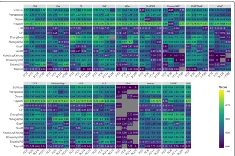
dimensional-ity reduction methods are summarized in Fig. 3 and

Additional file1: Figure S37-S54.

Trajectory inference by Slingshot

We first focused on the comparison results obtained from Slingshot. Different from the clustering results where accuracy generally increases with increasing num-ber of included low-dimensional components, the lineage tracing results from Slingshot do not show a clear increasing pattern with respect to the number of low-dimensional components, especially when we used k-means clustering as the initial step (Fig. 3 and

Add-itional file 1: Figure S39A). For example, the average

Kendall correlations across all data sets and across all methods are 0.35, 0.36, 0.37, and 0.37 for increasingly large number of components, respectively. When we used hierarchical clustering algorithm as the initial step, the lineage tracing results in the case of a small number of low-dimensional components are slightly inferior as compared to the results obtained using a large number

of low-dimensional components (Additional file 1:

Louvain method across all data sets and across all methods are 0.36, 0.38, 0.40, and 0.40 for increasingly large number of components, respectively. Therefore, Louvain method is recommended as the initial step for

lineage inference and a small number of

low-dimensional components there is often sufficient for ac-curate results. When conducting lineage inference based on a low number of components with Louvain method, we found that four dimensionality reduction methods, PCA, FA, ZINB-WaVE, and UMAP, all perform well for lineage inference across varying number of

low-dimension components (Additional file 1: Figure S39C).

For example, with the lowest number of components, the average Kendall correlations across data sets for PCA, FA, UMAP, and ZINB-WaVE are 0.44, 0.43, 0.40, and 0.43, respectively. Their performance is followed by

ICA (0.37), ZIFA (0.36), tSNE (0.33), and Diffusion Map (0.38), while pCMF (0.26), Poisson NMF (0.26), and LTSA (0.12) do not fare well.

Trajectory inference by Monocle3

We next examined the comparison results based on Monocle3 (Additional file 1: Figure S40-S41). Similar to Slingshot, we found that the lineage tracing results from Monocle3 also do not show a clear increasing pattern with respect to the number of low-dimensional compo-nents (Additional file 1: Figure S41). For example, the average Kendall correlations across all data sets and across all methods are 0.37, 0.37, 0.38, and 0.37 for an increasingly large number of components, respectively. Therefore, similar with Slingshot, we also recommend

the use of a small number of low-dimensional

components with Monocle3. In terms of dimensionality reduction method performance, we found that five di-mensionality reduction methods, FA, MDS, GLMPCA, ZINB-WaVE, and UMAP, all perform well for lineage inference. Their performance is often followed by NMF and DCA, while Poisson NMF, pCMF, LLE, and LTSA do not fare well. The dimensionality reduction compari-son results based on Monocle3 are in line with those recommendations by Monocle3 software, which uses UMAP as the default dimensionality reduction method [28]. In addition, the set of five top dimensionality re-duction methods for Monocle3 are largely consistent with the set of top five dimensionality reduction methods for Slingshot, with only one method difference between the two (GLMPCA in place of PCA). The simi-larity of top dimensionality reduction methods based on different lineage inference methods suggests that a simi-lar set of dimensionality reduction methods are likely suitable for lineage inference in general.

Visualization of inferred lineages

We visualized the reduced low-dimensional components from different dimensionality reduction methods in one trajectory data set, the ZhangBeta data. The ZhangBeta data consists of expression measurements on mouse pancreatic β cells collected at seven different develop-mental stages. These seven different cell stages include E17.5, P0, P3, P9, P15, P18, and P60. We applied differ-ent dimensionality reduction methods to the data to extract the first two-dimensional components. After-wards, we performed lineage inference and visualization using Monocle3. The inferred tracking paths are shown in Additional file1: Figure S42. Consistent with Kendall

correlation (Fig. 3), all top dimensionality reduction

methods are able to infer the correct lineage path. For example, the trajectory from GLMPCA and UMAP com-pletely matches the truth. The trajectory inferred from FA, NMF, or ZINB-WaVE largely matches the truth with small bifurcations. In contrast, the trajectory inferred from either Poisson NMF or LTSA displays un-expected radical patterns (Additional file1: Figure S42), again consistent with the poor performance of these two methods in lineage inference.

Normalization does not influence the performance of dimensionality reduction methods

For dimensionality reduction methods that require nor-malized data, we further examined the influence of differ-ent data transformation approaches on their performance (Additional file1: Figure S43-S53). Like in the clustering comparison, we found that different transformations do not influence the performance results for most dimension-ality reduction methods in lineage inference. For example,

in Slingshot with the k-means clustering algorithm as

the initial step, when the number of low-dimensional components is small, UMAP achieves a Kendall cor-relation of 0.42, 0.43, and 0.40, for log2 count

trans-formation, log2 CPM transtrans-formation, and z-score

transformation, respectively (Additional file 1: Figure S39A, S46A, and S50A). Similar results hold for the

hierarchical clustering algorithm (Additional file 1:

Figure S39B, S46B, and S50B) and Louvain method

(Additional file 1: Figure S39B, S46B, and S50B).

However, some notable exceptions exist. For example, with log2 CPM transformation but not the other transformations, the performance of Diffusion Map increases with increasing number of included

compo-nents when k-means clustering was used as the initial

step: the average Kendall correlations across different low-dimensional components are 0.37, 0.42, 0.44, and 0.47, re-spectively (Additional file1: Figure S43 and S46A). As an-other example, with z-score transformation but not with the other transformations, FA achieves the highest per-formance among all dimensionality reduction methods across different number of low-dimensional components (Additional file1: Figure S50A). Similarly, in Monocle3, dif-ferent transformations (log2 count transformation, log2

CPM transformation, and z-score transformation) do not

influence the performance of dimensionality reduction methods. For example, with the lowest number of low-dimensional components, UMAP achieves a Kendall correl-ation of 0.49, 0.47, and 0.47, for log2 count transformcorrel-ation, log2 CPM transformation, and z-score transformation, re-spectively (Additional file1: Figure S41, S53A, and S53B).

Stability analysis across data splits

We also investigated the stability and robustness of different dimensionality reduction methods by data split

in theHayashidata. We applied each dimensionality

MDS achieve a Kendall correlation of 0.75, 0.77, 0.77, and 0.78 averaged across the two subsets, respectively, and again with virtually no performance variability across data splits (Additional file1: Figure S54).

Overall, the results suggest that, in terms of downstream lineage inference accuracy and stability, the scRNA-seq non-specific dimensionality reduction method FA, PCA, and NMF are preferable across a range of data sets exam-ined here. The scRNA-seq-specific dimensionality reduc-tion methods ZINB-WaVE as well as the scRNA-seq non-specific dimensionality reduction method NMF are also preferable if one is interested in extracting a small number of low-dimensional components for lineage inference. In addition, the scRNA-seq-specific dimensionality reduction method Diffusion Map and scRNA-seq non-specific di-mensionality reduction method MDS may also be prefera-ble if one is interested in extracting a large number of low-dimensional components for lineage inference.

Large-scale scRNA-seq data applications

Finally, we evaluated the performance of different di-mensionality reduction methods in two large-scale scRNA-seq data sets. The first data is Guo et al. [68], which consists of 12,346 single cells collected through a non-UMI-based sequencing technique. Guo et al. data contains known cell cluster information and is thus used for dimensionality reduction method comparison based on cell clustering analysis. The second data is Cao et al. [28], which consists of approximately 2 million single cells collected through a UMI-based sequencing tech-nique. Cao et al. data contains known lineage informa-tion and is thus used for dimensionality reducinforma-tion method comparison based on trajectory inference. Since many dimensionality reduction methods are not scalable to these large-scale data sets, in addition to applying dimensionality reduction methods to the two data dir-ectly, we also coupled them with a recently developed

sub-sampling procedure dropClust to make all

dimen-sionality reduction methods applicable to large data [69]

(details in “Methods and Materials”). We focus our

comparison in the large-scale data using the k-means

clustering method. We also used log2 count trans-formation for dimensionality reduction methods that require normalized data.

The comparison results when we directly applied di-mensionality reduction methods to the Guo et al. data

are shown in Additional file 1: Figure S55. Among the

methods that are directly applicable to large-scale data sets, we found that UMAP consistently outperforms the remaining dimensionality reduction methods across a range of low-dimensional components by a large margin. For example, the average NMI of UMAP across different number of low-dimensional components (0.5%, 1%, 2%, and 3%) are in the range between 0.60 and 0.61

(Additional file 1: Figure S55A). In contrast, the average NMI for the other methods are in the range of 0.15– 0.51. In the case of a small number of low-dimensional components, we found that the performance of both FA and NMF are reasonable and follow right after UMAP. With the sub-sampling procedure, we can scale all di-mensionality reduction methods relatively easily to this large-scale data (Additional file 1: Figure S56). As a re-sult, several dimensionality reduction methods, most notably FA, can achieve similar or better performance as compared to UMAP. However, we do notice an appre-ciable performance loss for many dimensionality reduc-tion methods through the sub-sampling procedure. For example, the NMI of UMAP in the sub-sampling-based procedure is only 0.26, representing an approximately 56% performance loss compared to the direct application

of UMAP without sub-sampling (Additional file 1:

Figure S56 vs Figure S55). Therefore, we caution the use of sub-sampling procedure and recommend users to careful examine the performance of dimensionality reduction methods before and after sub-sampling to decide whether sub-sampling procedure is acceptable for their own applications.

For lineage inference in the Cao et al. data, due to computational constraint, we randomly obtained 10,000 cells from each of the five different developmental stages (i.e., E9.5, E10.5, E11.5, E12.5, and E13.5) and applied different dimensionality reduction methods to analyze the final set of 50,000 cells. Because most dimensionality reduction methods are not scalable even to these 50,000 cells, we only examined the performance of dimensional-ity reduction methods when paired with the sub-sampling procedure (Additional file1: Figure S57). With the small number of low-dimensional components, three dimensionality reduction methods, GLMPCA, DCA, and Isomap, all achieve better performance than the other dimensionality reduction methods. For example, with the lowest number of low-dimensional components, the average absolute Kendall correlations of GLMPCA, DCA, and Isomap are 0.13, 0.28, and 0.17, respectively. In contrast, the average absolute Kendall correlations of the other dimensionality reduction methods are in the

range of 0.01–0.12. With a higher number of

low-dimensional components, Isomap and UMAP show bet-ter performance. For example, with 3% low-dimensional components, the average absolute Kendall correlations of Isomap and UMAP increase to 0.17 and 0.30, respect-ively. Their performance is followed by Diffusion Map (0.15), ZINB-WaVE (0.14), and LLE (0.12), while the remaining methods are in the range of 0.04–0.07.

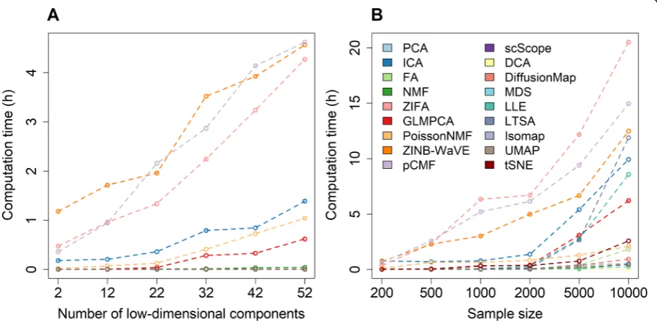
Computation time

Here, we also examined how computation time for differ-ent dimensionality reduction methods varies with respect to the number of low-dimensional components extracted (Fig.4a) as well as with respect to the number of cells con-tained in the data (Fig. 4b). Overall, the computational cost of three methods, ZINB-WaVE, ZIFA, and pCMF, is substantially heavier than that of the remaining methods. Their computation time increases substantially with both increasingly large number of low-dimensional compo-nents and increasingly large number of cells in the data. Specifically, when the sample size equals 500 and the de-sired number of low-dimensional components equals 22, the computing time for ZINB-WaVE, ZIFA, and pCMF to analyze 10,000 genes are 2.15, 1.33, and 1.95 h, respect-ively (Fig.4a). When the sample size increases to 10,000, the computing time for ZINB-WaVE, ZIFA, and pCMF increases to 12.49, 20.50, and 15.95 h, respectively (Fig.4b).

Similarly, when the number of low-dimensional compo-nents increases to 52, the computing time for ZINB-WaVE, ZIFA, and pCMF increases to 4.56, 4.27, and 4.62 h, respectively. Besides these three methods, the computing cost of ICA, GLMPCA, and Poisson NMF can also increase noticeably with increasingly large number of low-dimensional components. The comput-ing cost of ICA, but to a lesser extent of GLMPCA, LLE, LTSA, and Poisson NMF, also increases substan-tially with increasingly large number of cells. In con-trast, PCA, FA, Diffusion Map, UMAP, and the two deep-learning-based methods (DCA and scScope) are computationally efficient. In particular, the computa-tion times for these six methods are stable and do not show substantial dependence on the sample size or the number of low-dimensional components. Certainly, we expect that the computation time of all dimensionality

reduction methods will further increase as the sample size of the scRNA-seq data sets increases in magnitude. Overall, in terms of computing time, PCA, FA, Diffu-sion Map, UMAP, DCA, and scScope are preferable.

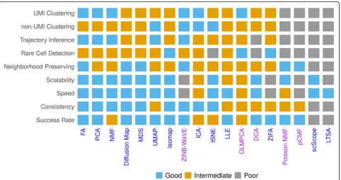
Practical guidelines

In summary, our comparison analysis shows that different dimensionality reduction methods can have different merits for different tasks. Subsequently, it is not straightforward to identify a single dimensionality reduction method that strives the best in all data sets and for all downstream ana-lyses. Instead, we provide a relatively comprehensive prac-tical guideline for choosing dimensionality reduction methods in scRNA-seq analysis in Fig. 5. Our guideline is based on the accuracy and effectiveness of dimensionality reduction methods in terms of the downstream analysis, the robustness and stability of dimensionality reduction methods in terms of replicability and consistency across data splits, as well as their performance in large-scale data applications, data visualization, and computational scalabil-ity for large scRNA-seq data sets. Briefly, for cell clustering analysis, PCA, ICA, FA, NMF, and ZINB-WaVE are recom-mended for small data where computation is not a concern. PCA, ICA, FA, and NMF are also recommended for large

data where computation is a concern. For lineage inference analysis, FA, PCA, NMF, UMAP, and ZINB-WaVE are all recommended for small data. A subset of these methods, FA, PCA, NMF, and UMAP are also recommended for large seq data. In addition, for very large scRNA-seq data sets (e.g., > 100,000 samples), DCA and UMAP perhaps are the only feasible approach for both down-stream analyses with UMAP being the preferred choice. We also recognize that PCA, ICA, FA, and NMF can be useful options in very large data sets when paired with a

sub-sampling procedure [69], though care needs to be

taken to examine the effectiveness of the sub-sampling pro-cedure itself. Finally, besides these general recommenda-tions, we note that some methods have additional features that are desirable for practitioners. For example, both ZINB-WaVE and GLMPCA can include sample-level and gene-level covariates, thus allowing us to easily control for batch effects or size factors. We provide our detailed rec-ommendations in Fig.5.

Discussion

We have presented a comprehensive comparison of dif-ferent dimensionality reduction methods for scRNA-seq analysis. We hope the summary of these state-of-the-art

dimensionality reduction methods, the detailed compari-son results, and the recommendations and guidelines for choosing dimensionality reduction methods can assist researchers in the analysis of their own scRNA-seq data.

In the present study, we have primarily focused on three clustering methods (k-means, hierarchical cluster-ing, and Louvain method) to evaluate the performance of different dimensionality reduction methods for down-stream clustering analysis. We have also primarily focused on two lineage inference methods (Slingshot and Monocle3) to evaluate the performance of different

dimensionality reduction methods for downstream

lineage inference. In our analysis, we found that the per-formance of dimensionality reduction methods mea-sured based on different clustering methods is often consistent with each other. Similarly, the performance of dimensionality reduction methods measured based on different lineage inference methods is also consistent with each other. However, it is possible that some di-mensionality reduction methods may work well with certain clustering approaches and/or with certain lineage inference approaches. Subsequently, future comparative analysis using other clustering methods and other lineage inference methods as comparison criteria may have added benefits. In addition, besides cell clustering and trajectory inference, we note that dimensionality re-duction methods are also used for many other analytic tasks in scRNA-seq studies. For example, factor models for dimensionality reduction is an important modeling part for multiple scRNA-seq data set alignment [16], for integrative analysis of multiple omics data sets [70,71], as well as for deconvoluting bulk RNA-seq data using cell type-specific gene expression measurements from scRNA-seq [72,73]. In addition, cell classification in scRNA-seq also relies on a low-dimensional structure inferred from original scRNA-seq through dimensionality reduction [74,

75]. Therefore, the comparative results obtained from the present study can provide important insights into these different scRNA-seq analytic tasks. In addition, investigat-ing the performance of dimensionality reduction methods in these different scRNA-seq downstream analyses is an important future research direction.

We mostly focused on evaluating feature extraction methods for dimensionality reduction. Another important category of dimensionality reduction method is the feature selection method, which aims to select a subset of fea-tures/genes directly from the original feature space. The feature section methods rely on different criteria to select important genes and are also commonly used in the pre-processing step of scRNA-seq data analysis [76]. For ex-ample, M3Drop relies on dropout events in scRNA-seq data to identify informative genes [77]. Seurat uses gene expression variance to select highly variable genes [16]. Evaluating the benefits of different methods and criteria

for selecting informative genes for different downstream tasks is another important future direction.

We have primarily focused on using the default soft-ware settings when applying different dimensionality re-duction methods. We note, however, that modifying the software setting for certain methods on certain data types may help improve performance. For example, a re-cent study shows that the quasi-UMI approach paired with GLMPCA may help improve the performance of

GLMPCA on non-UMI data sets [78]. In addition, we

have relied on a relatively simple gene filtering step by removing lowly expressed genes. Sophisticated gene filtering approaches prior to running dimensionality reduction may help improve the performance of certain dimensionality reduction methods. In addition, alternative, more stringent gene filtering approaches may likely result in a smaller subset of genes for per-forming dimensionality reduction, making it easier to apply some of the slow dimensionality reduction methods to large data sets. Exploring how different software settings and gene filtering procedures influ-ence the performance of different dimensionality re-duction methods on different data sets will help us better understand the utility of these methods.

With the advance of scRNA-seq technologies and with the increase collaborations across scientific groups, new consortium projects such as the Human Cell Atlas (HCA) will generate scRNA-seq data sets that contain millions of cells [34]. The large data at this scale poses critical compu-tational and statistical challenges to many current dimen-sionality reduction methods. Many existing dimendimen-sionality reduction methods, in particular those that require the computation and memory storage of a covariance or dis-tance matrix among cells, will no longer be applicable there. We have examined a particular sub-sampling strat-egy to scale all dimensionality reduction methods to large data sets. However, while the sub-sampling strategy is computationally efficient, it unfortunately reduces the per-formance of many dimensionality reduction methods by a substantial margin. Therefore, new algorithmic innova-tions and new efficient computational approximainnova-tions will likely be needed to effectively scale many of the existing dimensionality reduction methods to millions of cells.

Methods and materials ScRNA-seq data sets

We obtained a total of 30 scRNA-seq data sets from public domains for benchmarking dimensionality re-duction methods. All data sets were retrieved from the

Gene Expression Omnibus (GEO) database (https://

(8 data sets), 10X Genomics (6 data sets), Smart-Seq (5 data sets), inDrop (1 data set), RamDA-seq (1 data set), sci-RNA-seq3 (1 data set), SMARTer (5 data sets), and others (3 data sets). In addition, these data cover a range of sample sizes from a couple hundred cells to tens of thousands of cells measured in either human (19 data sets) or mouse (11 data sets). In each data set, we evaluated the effectiveness of different dimensional-ity reduction methods for one of the two important downstream analysis tasks: cell clustering and lineage inference. In particular, 15 data sets were used for cell clustering evaluation while another 15 data sets were used for lineage inference evaluation. For cell cluster-ing, we followed the same criteria listed in [12, 41] to select these datasets. In particular, the selected data sets need to contain true cell clustering information which is to be treated as the ground truth in the comparative analysis. In our case, 11 of the 15 data sets were ob-tained by mixing cells from different cell types either pre-determined by fluorescence activated cell sorting (FACS) or cultured on different conditions. Therefore, these 11 studies contain the truecell type labels for all cells. The remaining 4 data sets contain cell labels that were determined in the original study and we simply treated them as truth though we do acknowledge that such“true” clustering information may not be accurate. For lineage inference, we followed the same criteria listed in [14] to select these datasets. In particular, the selected data sets need to contain true linear lineage in-formation which is to be treated as the ground truth in the comparative analysis. In our case, 4 of the 15 data sets were obtained by mixing cells from different cell types pre-determined by FACS. These different cell types are at different developmental stages of a single

linear lineage; thus, these 4 studies contain the true

lineage information for all cells. The remaining 11 data sets contain cells that were collected at multiple time points during the development process. For these data, we simply treated cells at these different time points as part of a single linear lineage, though we do acknow-ledge that different cells collected at the same time point may represent different developmental trajector-ies from an early time point if the cells at the early time are heterogeneous. In either case, the true lineages in all these 15 data sets are treated as linear, without any bifurcation or multifurcation patterns.

A detailed list of the selected scRNA-seq datasets with corresponding data features is provided in Additional file1: Table S1-S2. In each of the above 30 data sets, we re-moved genes that are expressed in less than five cells. For methods modeling normalized data, we transformed the

raw counts data into continuous data with thenormalize

function implemented in scater(R package v1.12.0). We

then applied log2 transformation on the normalized

counts by adding one to avoid log transforming zero values. We simply term this normalization as log2 count transformation, though we do acknowledge that such transformation does take into account of cell size factor, etc. through thescatersoftware. In addition to log2 count transformation, we also explored the utility of two add-itional data transformation: log2 CPM transformation and z-score transformation. In the log2 CPM transformation, we first computed counts per million reads (CPM) and then performed log2 transformation on the resulted CPM value by adding a constant of one to avoid log transform-ation of zero quantities. In thez-score transformation, for each gene in turn, we standardized CPM values to achieve a mean of zero and variance of one across cells using Seu-ratpackage (v2.3).

Besides the above 30 real scRNA-seq data sets, we also simulated 2 additional scRNA-seq data sets for cell clus-tering evaluation. In the simulations, we used all 94 cells

from one cell type (v6.5 mouse 2i+LIF) in the Kumar

data as input. We simulated scRNA-seq data with 500 cells and a known number of cell types, which were set to be either 4 or 8, using theSplatterpackage v1.2.0. All parameters used in the Splatter (e.g., mean rate, shape, dropout rate) were set to be approximately those esti-mated from the real data. In the case of 4 cell types, we set the group parameter inSplatteras 4. We set the per-centage of cells in each group as 0.1, 0.15, 0.5, and 0.25, respectively. We set the proportion of the differentially expressed genes in each group as 0.02, 0.03, 0.05, and 0.1, respectively. In the case of 8 cell types, we set group/cell type parameter as 8. We set the percentage of cells in each group as 0.12, 0.08, 0.1, 0.05, 0.3, 0.1, 0.2, and 0.05, respectively. We set the proportion of the dif-ferentially expressed genes in each group as 0.03, 0.03, 0.03, 0.1, 0.05, 0.07, 0.08, and 0.1, respectively.

Compared dimensionality reduction methods

Dimensionality reduction methods aim to transform an originally high-dimensional feature space into a low-dimensional representation with a much-reduced number of components. These components are in the form of a linear or non-linear combination of the original features (known as feature extraction dimensionality reduction methods) [79] and in the extreme case are themselves a subset of the ori-ginal features (known as feature selection dimensionality

re-duction methods) [80]. In the present study, we have

Kullback-Leibler divergence-based NMF (Poisson NMF; R package NNLM, v1.0.0), zero-inflated factor analysis (ZIFA;

Python package ZIFA), zero-inflated negative

binomial-based wanted variation extraction (ZINB-WaVE; R package zinbwave, v1.6.0), probabilistic count matrix factorization (pCMF; R package pCMF, v1.0.0), deep count autoencoder

network (DCA; Python package dca), a scalable

deep-learning-based approach (scScope; Python packagescscope), generalized linear model principal component analysis (GLMPCA; R package on github), multidimensional scaling (MDS; Rdimtools R package v.0.4.2), locally linear embed-ding (LLE; Rdimtools R packge v.0.4.2), local tangent space alignment (LTSA; Rdimtools R package v.0.4.2), Isomap (Rdimtools R package v.0.4.2), t-distributed stochastic

neigh-bor embedding (tSNE; FIt-SNE, fftRtnse R function), and

uniform manifold approximation and projection (UMAP; Python package). One of these methods, tSNE, can only ex-tract a maximum of two or three low-dimensional compo-nents [48,58,59]. Therefore, we only included tSNE results based on two low-dimensional components extracted from the recently developed fast FIt-SNE R package [48] in all figures. An overview of these 18 dimensionality reduction methods with their corresponding modeling characteristics is provided in Table1.

Assess the performance of dimensionality reduction methods

We first evaluated the performance of dimensionality re-duction methods by neighborhood preserving that aims to access whether the reduced dimensional space resem-bles the original gene expression matrix. To do so, we first identified the k-nearest neighbors for each single cell in the original space (denoted as a set A) and in the reduced space (denoted as a set B). We setk= 10, 20, or 30 in our study. We then computed the Jaccard index (JI) [60] to measure the neighborhood similarity between the original space and the reduced space: JI¼j_jA_A∩_∪B_Bj_j, where |∙| denotes the cardinality of a set. We finally ob-tained the averaged Jaccard index (AJI) across all cells to serve as the measurement for neighborhood preserving. We note, however, that neighborhood preserving is pri-marily used to measure the effectiveness of pure dimen-sionality reduction in terms of preserving the original space and may not be relevant for single-cell analytic tasks that are the main focus of the present study: a di-mensionality reduction method that preserve the original gene expression matrix effectively may not be effective in extracting useful biological information from the ex-pression matrix that are essential for key downstream single-cell applications. Preserving the original gene ex-pression matrix is rarely the purpose of dimensionality reduction methods for single-cell applications: indeed, the original gene expression matrix (which is the

best-preserved matrix of itself) is rarely, if ever, used directly in any downstream single-cell applications including cell clustering and lineage inference, even though it is com-putationally easy to do so.

Therefore, more importantly, we also evaluated the performance of dimensionality reduction methods by evalu-ating how effective the low-dimensional components ex-tracted from dimensionality reduction methods are for downstream single-cell analysis. We evaluated either of the two commonly applied downstream analysis, clustering analysis, and lineage reconstruction analysis, in the 32 data sets described above. In the analysis, we varied the number of low-dimensional components extracted from these di-mensionality reduction methods. Specifically, for cell clus-tering data sets, in a data with less than or equal to 300 cells, we varied the number of low-dimensional compo-nents to be either 2, 6, 14, or 20. In a data with more than 300 cells, we varied the number of low-dimensional com-ponents to be either 0.5%, 1%, 2%, or 3% of the total num-ber of cells. For lineage inference data sets, we varied the number of low-dimensional components to be either 2, 6, 14, or 20 for all data sets, since common lineage inference methods prefer a relatively small number of components.

For clustering analysis, after dimensionality reduction with these dimensionality reduction methods, we used three different clustering methods, the hierarchical clus-tering (R functionhclust; stats v3.5.3), k-means clustering (R function kmeans; stats v3.6.0), or Louvain method (R functionclusterCells; monocle v2.12.0) to perform cluster-ing on the reduced feature space. Thek-means clustering is a key ingredient of commonly applied scRNA-seq clus-tering methods such as SC3 [18] and Waterfall [25]. The hierarchical clustering is a key ingredient of commonly applied scRNA-seq clustering methods such as CIDR [17]

and CHETAH [81]. The Louvain method is also a

com-monly used clustering method for common single-cell analysis software such as Seurat [16] and Monocle [27,

82]. In all these clustering methods, we set the number of

clusters k to be the known number of cell types in the

data. We compared the cell clusters inferred using the low-dimensional components to the true cell cluster and evaluated clustering accuracy by two criteria: the adjusted rand index (ARI) [83] and the normalized mutual infor-mation (NMI) [84]. The ARI and NMI are defined as:

ARIðP;TÞ ¼

P

l;s nls

2

−½P_l al

2

P

s bs

2 =

n 2

1 2½

P

l al

2 þ

P

s bs

2 −½

P

l al

2

P

s bs

2 =

n 2

andNMIðP;TÞ ¼_H2_ðMI_PÞþðP_H;T_ðTÞ_Þ;

where P= (p1,p2,⋯,pn)T denotes the inferred cell type