EFFECT OF SECOND ORDER SLIP ON FLOW AND HEAT TRANSFER CHARACTERISTICS OF A VISCOUS FLUID OVER A SHRINKING SHEET

EFFECT OF SECOND ORDER SLIP ON FLOW AND HEAT

TRANSFER CHARACTERISTICS OF A VISCOUS FLUID OVER A

SHRINKING SHEET

Muneer Patel

Department of Mathematics, Dravidian University, Kuppam-517425, Andra Pradesh, India

ABSTRACT

This paper considers the study of viscous flow and heat transfer over a shrinking sheet

considering the effect of second order slip. The governing partial differential equations of the

flow and heat transfer are converted into nonlinear ordinary differential equations by using

suitable similarity transformation. The exponential form of solution for momentum equation is

assumed and governing heat transfer equation is solved analytically by power series method

and the solution is obtained in terms of Kummer’s Hypergeometric function. The effects of

various physical parameters on flow and heat transfer characteristics are investigated with

graphical illustrations.

Keywords: Shrinking sheet, Second Order Slip, Kummer’s Function, Mass suction

1.Introduction

The flow induced by a moving boundary is important in the study of extrusion processes

(Sakiadis B.C. 1961). (Sakiadis B.C.1961). (Crane L .J, 1970) and is a subject of considerable

interest in the contemporary literature (Miklavcic M, Wang CY, 2006), for both permeable and

impermeable stretching sheets. Miklavcic and Wang ( Miklavcic M, Wang C.Y.2006).have

reported an exact solution of the NS equations for flow over a shrinking sheet. The shrinking

sheet problem was also extended to power-law shrinking velocity and other fluids.

International Research Journal of Natural and Applied Sciences ISSN: (2349-4077) Impact Factor- 5.46, Volume 4, Issue 10, October 2017 Website- www.aarf.asia, Email : [email protected] , [email protected]

In the past decade, fluid flow in micro-electro-mechanical systems (MEMS) has become a hot

research topic. Because of the micro-scale dimensions of these devices, the flow behaviuor

deviates significantly from the traditional no-slip flow (Gal-el-Hak M, 1999). Rarefied gas flows

with slip boundary conditions are often encountered in micro-scale devices and low-pressure

situation (Gal-el-Hak M, 1999).

For the flow in the slip regime (Shidlovskiy VP.1967 and Pande GC, Goudas CL 1996)., the

fluid motion still obeys the Navier-Stokes (NS) equations with slip velocity boundary

conditions. In addition, partial slip over moving surface also occurs for fluids with particulate

such as emulsions, suspensions, foams, and polymer solutions (Yoshimura A, proteome

RK,1988),the slip flows under different flow configurations have been studied in recent years.

However, in these papers, only the first order Maxwell slip condition was used. Recently, (Wu

L.A, 2008) proposed a new second order slip velocity model, which matches with the

Fukui-Kaneko results based on the direct numerical simulation of the linerized Boltzmann equation

(Fukui S, Kaneko R. A, 2009.). (Tiegang Fang, Shanshan Yao, ji Zzhang, Abdul Aziz, 2009)

Studied the slip flow over a permeable shrinking surface with the newly proposed Wu’s slip

velocity model with exact solutions of the governing NS equations. In the present study we have

extended the work of (Tiegang Fang, Shanshan Yao, ji Zzhang, Abdul Aziz ,2009) considering

heat transfer and also with boundary layer approximation.

2. Mathematical formulation and discussion

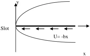
Consider a steady, two-dimensional laminar flow over a continuously shrinking sheet in a

quiescent fluid. The sheet shrinking velocity is Uw = - U0 x , with U0 being a constant and the wall

mass transfer velocity is Vw =Vw (x), which will be determined later.

Fig (1): Schematic diagram of boundary layer slip flow past a shrinking sheet

U= -bx Slot

y

x

The x-axis runs along the shrinking surface in the direction opposite to the sheet motion

and the y-axis is perpendicular to it. The governing boundary layer equation for the proposed

problem can be expressed as

0 u v x y       (1) 2 2

u u u

u v v

x y y

 

 _  

  

  _ _

(2)

With the boundary conditions

U(x, 0) = U0 x+Uslip, V(x, 0) = Uw (x), and u(x,) = 0,

(3)

Where u and v are the velocity components in the x and y directions. v is the kinematic

coefficient of viscosity,  is the fluid density, and Uslip is the velocity slip at the wall. The

Wu’s slip velocity model used in this paper is valid for arbitrary Knudsen numbers, Kn, and is

given as follows (Wu ,2008)

Uslip =





3 2 2 2

4 2 2

2 2 2

2 3 3 1 1 2

1 ,

3 2 _n 4 _n

l l u u u u

l l A B

K y K y y y

 _{ }



  _    _  _{ }   _  _ 

  _   _{  }

    (4)

Where l = min [ 1

n

K , 1], , is the momentum accommodation coefficient with 0    1, and

 is the molecular mean free path. Based on the definition of l, it is noticed that any given value of Kn, we have

0  l  1. The molecular mean free path is always positive. Thus we know that B0 and

positive. The stream function and similarity variable can be assumed in the following form,

 

    U0

y







(5)

With these transformations, the velocity components are expressed as

'

0 ( )

uU xf  andv  U v f0 ( ) .

The wall mass transfer velocity becomesvw( )x   U v f0 (0).

(7)

Using equations (5) and (6) in equations (1) and (2) we obtain the transformed form of boundary

layer equations of motion,

''' '' '2

0

f  ff  f  (8)

Similarly, the boundary conditions equation (3) takes the form

(0) ,

f s f'(0)  1  f//(0) f///(0)0, and f'( ) 0, (9) Where s is the wall mass transfer parameter showing the strength of the mass transfer at the

surface,  is the first order velocity slip parameter with 0

0 A U ,

v

 

 and  is the second

order velocity slip parameter with 0

0 BU .

v

 

 we derive a closed form exact solution of

Eq.(8) subject to the BCs of Eq. (9). We assume a solution of the form f( )  a be. The application of boundary condition (9) gives the values for a and b as mentioned below.

2 3

1

b

  



  ,

(10)

2 3

1

a S

  

 

  ,

(11)

Substituting the assumed solution into Eq.(9) yields a = . The use of this relationship in Eq.

(11) leads to the following fourth order algebraic equation for ,

4 3 2

( s) ( s 1) s 1 0

            .

(12)

 should be least positive value.

Then the solution reads as

2 3 2 3

1 1

( )

f  s e 

     



  

    ,

2

1 ( )

1

f  e 

  

 

  ,

(14)

Based on the results in Eq. (14), it is easy to show that

// 2

2

(0) ( )

1

f   s 

 

  

 

(15)

3. Heat transfer analysis

The thermal boundary layer equation, with work done by deformation, and internal heat

generation or absorption is given by

2

2

p

T T k T

u v

x y c y

  

 

  

(16)

Where cp is the specific heat,  is density, k is thermal conductivity

3.1 Constant surface temperature (CST)

The boundary conditions in case of CST is given by

at 0; as

w T T y

T T_ y

 

  

(17)

Where T_W is the temperature of the sheet and T_ is the temperature of the fluid far away from

the sheet.

Defining the non-dimensional temperature  

 

 

Using ( 18), Eq. (16 ) can be written in the form

 

   

'' '

Pr f 0

      

(19)

Where Pr Cp

k



Consequently the boundary conditions (17) take the form

 

 

Introducing the new independent variable

Pre 

 _{ } 

and substituting in Eq. (19) we obtain

 

 

 

 

'' ' ' '

11 12 0

P P

          

(21)

Where 11 12

Pr

, Pr

a b

P P and  e 

 



  

The corresponding boundary conditions are

 

 

The solution of Eq. (21) subject to the boundary conditions (22) is given by

 

1

Pr Pr

Pr 1 , ; Pr

k

a b a

C e  M k k e 

                _ _ _   _{  }  _            (23) Where 1 Pr 1 Pr Pr

Pr 1 ,

k C

a b a

e  M k k

     _{    }   _   _{  }  _   _{    }  

3.2 The Prescribed surface temperature (PST case)

2

0

W

x

T T T A at y l

T T at y

        _{ }        _{  } (24)

Where A is constant. T_W is temperature at the wall. T_ is temperature away from the sheet.

We define non-dimensional temperature as

 

So that the equation (16) reduces to the form

 

   

   

'' ' '

Pr 2f Pr f

         

(26)

the corresponding boundary conditions (24) reduces to

0 1 0           _{ } (27)

Using the new independent variable defined as

2 Pre t     

and substituting in equation (26) we obtain

 





 

'' '

11 12

1 2 0

t t  P P t  t   

(28)

WhereP₁₁ aPr , P₁₂ b



 

The corresponding boundary conditions will be

 

 

1 Pr

0 0

t at t e

t as t

    _    _   _{ } (29)

We obtain the solution of above equation (26) by using power series method and in terms of

 

Pr Pr

2

Pr Pr Pr

2 2 , 1 ,

Pr Pr Pr

2 2 , 1 ,

a a a

e M b e

a a

M b

 _{ }

  

 

 

  

  _  _   _    

     

   

 



 _  _   _   

     

   

 

(30)

4. Results and Discussion

In this problem, we proposed to investigate the flow and heat transfer characteristics of a

viscous fluid with second order slip. The governing equations for momentum and heat transfer

are partial differential equations which are converted into ordinary differential equations by

using suitable similarity transformations.

An analytical solution [exponential solution] for flow has been assumed, and this assumed

solution is used to solve the heat transfer equations by power series method and expressed in

terms of Kummer’s hyper geometric functions. The results are depicted graphically from graph

Fig 2 to 12.

Fig 2. Shows the effect of mass suction parameter s on considered flow. It shows that as there is

increase in the parameter value of‘s’ velocity '

f is decreases.

Fig 3. Shows the effect of first order slip parameter  on velocity profile f'. It is noticed that as

first order slip parameter  increases velocity profile f' decreases.

Similarly in Fig 4, we notice that the effect of second order slip parameter is to sustain velocity

profile f' in the boundary layer.

Fig (5) and (6), Shows the effect of mass suction parameter on temperature profile in CST and

PST cases. It is observed from these two graphs that as mass suction parameter s increases

temperature decreases.

Fig (7) and (8), Shows the effect of second order slip parameter in CST and PST cases. It is

observed from these two graphs that as decreases temperature increases.

Fig. (9) and (10), Shows the effect Pr in CST and PST cases. It is observed from these two

Fig (11) and (12), Shows the effect of first order slip parameter  .in CST and PST cases. It is

observed from these two graphs that as increases temperature decreases.

Nomenclature

x flow directional coordinate along the stretching sheet

y distance normal to the stretching sheet

u, v velocity components along x and y direction

a, b constants

 root value

 first order velocity slip parameter  second order velocity slip parameter

A prescribed constants

p

c specific heat at constant pressure

k thermal Conductivity

T fluid temperature of the moving sheet

w

T wall temperature

Pr Prandtl number

T_ temperature far away from the plate

w

 wall shearing stress

s mass suction

M Kummer’s Function

Greek symbols

 dimensionless temperature

 dimensionless space variable

 Kinematic viscosity

 density

 coefficient of viscosity

Subscripts

w properties at the plate

η differentiation with respect to η

References

[1] Sakiadis B.C., 1961. Boundary-layer behavior on continuous solid surface: I. Boundary-layer

equations for two-dimensional and axisymmetric flow Aiche :26-8.

[2]Sakiadis B.C.1961. Boundary-layer behavior on continuous solid surface: II. Boundary-layer

equations for two-dimensional and axisymmetric flow A .I .C .H. E :7:221-5.

[3] Crane L ,J. 1970. Flow past a stretching plate. Z Angew Maths phys .21 {4}; 645.

[4] Miklavcic M, Wang CY.2006. Viscous flow due to a shrinking sheet. Quart Appl Math

64(2); 283-90

[5] Fang T. 2008.Boundary layer flow over a shrinking sheet with power- law velocity.

Int J Heat Mass Transfer 51(25/26); 5838-43.

[6] Fang T, Zhang J. 2009.Closed-form exact solutions of MHD Viscous flow over a shrinking

Sheet. Comm.Nonlin .Sci.numer. simul ; 14(7); 2853-2857.

[7]Fang T, Zhang J, Yao S.2009. Viscous flow over an unsteady shrinking sheet with mass

transfer. Chin Phys Lett 26(1); 014703.

[8]Fang T, Liang W, Lee CF. 2008.A new solutions branch for the blasius equation – a

shrinking sheet problem. Comp Math Appl56 (12); 3088-95.

[9]Fang T, Zhang J, 2009.Heat transfer over a shrinking sheet – an analytical solution.

Acta Mech. Doi; 10.1007/s00707-009-0183-2;

[10] Hayat T, Abbas Z, Sajid M.2007. On the analytic solution of magneto hydrodynamic flow

of a second grade fluid over a shrinking sheet Appl Math Trans ASME 74(6); 1165-71.

[11] Sajid M, Hayat T, Jived T. 2008. MHD rotating flow of a viscous fluid over a shrinking

surface. Nonlinear Dyn 51(1-2); 259-65.

[12]Sajid M, Hayat T, 2007. The application of homotopy analysis method for MHD viscous

flow due to a shrinking sheet. Chaos, solutions & Fractals doi;10,1016/j.chaos.2007.06.019.

[13]Elbashbeshy EMA,1998. Heat transfer over a stretching with variable surface heat flux.

JPhys D Appl Phys31; 1951-4.

[14] Magyari E, Keller B1999. Heat and mass transfer in the boundary layers on an

exponentially stretching continuous surface. J Phys D Appl Phys 32 ;( 5); 577- 585.

[16]Magyari E, Ali ME, Keller B. 2001.Heat and mass transfer characteristics of the self-

similar boundary-layer flows induced by continuous surfaces stretched with rapidly

decreasing velocities. Heat Mass Transfer 38(1-2); 65-74.

[17]Liao S.J.2005. A new branch of solutions of boundary-layer flows over a stretching flat

plate. Int Heat Mass Transfer 49(12); 2529-39.

[18] Liao S.J, 2007. A new branch of solutions of boundary-layer flows over a permeable

stretching plate. Int J Nonlinear Mech 42; 819-30

[19]Fang T, Zhang J, 2008.Flow between two stretchable disks. Int common Heat Mass

transfer 35(8); 892-5.

[20] Fang T.2007. Flow over a stretchable disk. Phys Fluids 19; 128105.

[21]Wang C.Y.1991. Exact solutions of the steady state navier-stokes equations. Ann Rew

Fluid Mech 23:159-77.

[22]Miklavcic M, Wang C.Y.2006. Viscous flow due to a shrinking sheet. Quart Appl Math

64(2); 283-90

[23]Fang T.2008. Boundary layer flow over a shrinking sheet with power- law velocity. Int J

Heat Mass Transfer 51(25/26); 5838-43.

[24]Fang T, Zhang J. 2009. Closed-form exact solutions of MHD Viscous flow over a

shrinking sheet. Commun Nonlinear Sci numer simulate 14(7); 2853-7.

[25]Fang T, Zhang J, Yao S.2009. Viscous flow over an unsteady shrinking sheet with mass

transfer. Chin Phys Lett 26(1); 014703.

[26]Fang T, Liang W, Lee CF. 2008.A new solutions branch for the blasius equation – a

shrinking sheet problem. Comut Math Appl 56(12); 3088-95.

[27]Fang T, Zhang J, 2009.Heat transfer over a shrinking sheet – an analytical solution. Acta

Mech. Doi; 10.1007/s00707-009-0183-2.

[28]Hayat T, Abbas Z, Sajid M.2007.on the analytic solution of magneto hydrodynamic flow

of a second grade fluid over a shrinking sheet. Apple Meth Trans ASME 74(6); 1165-71.

[29]Sajid M, Hayat T, jived T. 2008.MHD rotating flow of a viscous fluid over a shrinking

surface. Nonlinear Dyn 51(1-2); 259-65.

[30]Sajid M, Hayat T, 2007.The application of homotopy analysis method for MHD viscous

flow due to a shrinking sheet. Chaos, solutions & Fractsls doi;10,1016/j.chaos.

[31] Gal-el-Hak M.1999. The fluid mechanics of micro-devices-the freeman scholar. ASME

[32] Shidlovskiy VP.1967. Introduction to the dynamics of rarefied gases. New York;

American Elsevier publishing company Inc

[33] Pande GC, Goudas CL.1996. Hydro magnetic Rayleigh problem for a porous wall in slip

flow regime. Astrophys Space Sci 243:285-9.

[34]Yoshimura A, proteome RK. 1998. Wall slips correction for coquette and parallel disc

viscometers. J Rheol 32; 53-67.

[35]Martin MJ, Boyd ID.2001. Blasius boundary layer solution with slip flow conditions. In:

AIP conference proceedings, rarefied gas dynamics: 22nd international symposium,

vol. 585, .p. 518-23.

[36]Anderson HI.2002. Slip flow past a stretching surface. Acta Mech 158:121-5.

[37]Wang CY.2002. Flow due to a stretching boundary with partial slip-an exact solution of

the Navier-stokes equations. Chem Eng Sci 57(17); 3745-7.

[38]Fang T, Lee CF.2005. A moving-wall boundary layer flow of a slightly rarefied gas free

stream over a moving flat plate. Apple Math Lett. 18 ;( 5); 487-95.

[39]Fang T, Lee CF.2006. exact solutions of incompressible coquette flow with porous walls

for slightly rarefied gases. Heat mass transfer .42(3); 255-62.

[40] Fang T, Zhang J, Yao S.2009. Slip MHD viscous flow over a stretching sheet – an exact

solution. Commum Nonlinear Sci numer simulat 14(11); 3731-7

[41]Wang CY., 2006. Stagnation slip flow and heat transfer on a moving plate. Chem. eng sci

61(23); 7668-72.

[42]Wang CY2007.stagnation flow on a cylinder with partial slip – an exact solution of the

Navier-stokes equations. IMA J Apple Math 72(3); 271-7.

[43] Wang CY.2009. Analysis of viscous flow due to a stretching sheet with surface slip and

suction. Nonlinear Anal Real world Apple, 10(1); 375-80.

[44]Aziz A. 2009.Hydrodynamic and thermal slip flow boundary layers over a flat plate with

constant heat flux boundary condition. Commun Nonlinear sci numer simulate. Doi;

10.1016/j.cnsns

[45]Wu L.A slip model for rarefied gas flows at arbitrary Knudsen number. Appl Phys

lett 2008; 93:253103.

[46]Tiegang Fang, Shanshan Yao, ji Zzhang, Abdul Aziz 2009, viscous flow over a shrinking

0 1 2 3 4 5 -0.30

-0.25 -0.20 -0.15 -0.10 -0.05 0.00

Fig(2) Variation of f'() versus  for different values of s



f'()

Velocity Profile

=-1.0,

=1.0

s=3,2,1

0.0 0.5 1.0 1.5 2.0 2.5 3.0 3.5 4.0

-0.08 -0.07 -0.06 -0.05 -0.04 -0.03 -0.02 -0.01 0.00 0.01

Fig(3) Variation of f'() versus  for different values of 



f'()

Velocity Profile s=2.0, = -0.03

0 2 4 6 8 10 0.0

0.2 0.4 0.6 0.8 1.0

Fig(5) Variation of () versus for different values of s s=1,2,3

 ()

CST CASE Pr=1,=1,=-1

0 1 2 3 4

-0.05 -0.04 -0.03 -0.02 -0.01 0.00

Fig(4) Variation of f'() versus  for different values of 

Velocity Profile s=2, = 0.5

f'()



0 2 4 6 0.0

0.2 0.4 0.6 0.8

1.0 PST CASE

= -1.0, = 1.0, Pr= 1.0

s= 1, 2, 3, 4, 5

Fig(6) Variation of ()versus for different values of s

 

0 2 4 6 8 10

0.0 0.2 0.4 0.6 0.8 1.0

()



Fig(7) Variation of ()versus for different valuses of  =-1,-2,-3

0 2 4 6 8 10 0.0

0.2 0.4 0.6 0.8 1.0

Fig(9) Variation of ()versus for different valuses of Pr Pr=0.7,1.0,1.5

cst case

=1.0, =1.0, s=1.0

()



0 2 4 6 8 10

0.0 0.2 0.4 0.6 0.8 1.0

Fig(8) Variation of ()versus for different valuses of 



 = -1,-2,-3,-4,-5

0 1 2 3 4 5 6 0.0

0.2 0.4 0.6 0.8 1.0

Fig(10) Variation of() versus for different valuses of Pr





PST CASE

= -1.0, = 1.0, s= 1.0

Pr=0.7, 1, 1.5, 2, 2.5

0 2 4

0.0 0.2 0.4 0.6 0.8 1.0

Fig(11) Variation of ()versus for different valuses of  CST CASE S=1,Pr=1,=1

=3,5,7

0 2 4 6 8 10 0.0

0.2 0.4 0.6 0.8 1.0

Fig(12) Variation of()versus for different valuses of 

PST CASE

S=1,Pr=1,=-1

 ()