R E S E A R C H
Open Access
A modified nonmonotone BFGS algorithm
for unconstrained optimization
Xiangrong Li
*, Bopeng Wang and Wujie Hu
*Correspondence: [email protected]
Guangxi Colleges and Universities Key Laboratory of Mathematics and Its Applications, College of Mathematics and Information Science, Guangxi University, Nanning, Guangxi, P.R. China
Abstract
In this paper, a modified BFGS algorithm is proposed for unconstrained optimization. The proposed algorithm has the following properties: (i) a nonmonotone line search technique is used to obtain the step size
α
kto improve the effectiveness of the algorithm; (ii) the algorithm possesses not only global convergence but also superlinear convergence for generally convex functions; (iii) the algorithm produces better numerical results than those of the normal BFGS method.MSC: 65K05; 90C26
Keywords: BFGS update; global convergence; superlinear convergence; nonmonotone
1 Introduction
Consider
minf(x)|x∈ n, (.)
wheref(x) :n→ is continuously differentiable. Many similar problems can be trans-formed into the above optimization problem (see [–] etc.). The following iteration for-mula is used to address the iteration point of (.):
xk+=xk+αkdk, k= , , , . . . , (.)
wherexkis thekth iterative point,αk> is the step length, anddkis the search direction off atxk. The search directiondkdetermines the line search method (see [–]). The quasi-Newton method is defined by
Bkdk+gk= , (.)
wheregk=∇f(xk),Bkis the quasi-Newton update matrix, and the sequence{Bk}satisfies the so-called quasi-Newton equation
Bk+sk=yk, (.)
wheresk=xk+–xk,yk=gk+–gk, andgk+=∇f(xk+). The following update ofBk:
Bk+=Bk–
BksksTkBk
sTkBksk +yky
T k
sTkyk
(.)
is the BFGS formula (Broyden [], Fletcher [], Goldfar [], and Shanno []), which is one of the most effective quasi-Newton methods. Convex functions can be combined with exact line or certain special inexact line search techniques that have global convergence (see [–] etc.) and superlinear convergence (see [, ] etc.). For general functions, under inexact line search techniques, Dai [] constructed an example to show that the BFGS method fails. Mascarenhas [] proved the nonconvergence of this method, even with the exact line search technique. To obtain global convergence of a BFGS method with-out the convexity assumption, Li and Fukushima [, ] proposed the following modified BFGS methods.
Formula ([]) The BFGS update formula is defined by
Bk+=Bk+
δTkδk
sTkδk
–Bksks T kBk
sTkBksk
, (.)
whereδk=yk+ (max{, – yTksk
sk}+φ(gk))skand functionφ: → satisfies: (i)φ(t) >
for allt> ; (ii)φ(t) = if and only ift= ; (iii) iftis in a bounded set, andφ(t) is bounded. Using the definition ofδk, it is not difficult to obtain
δTksk≥max
sTkyk,φ
gk
sk
> .
This is sufficient to guarantee the positive definiteness ofBk+ as long asBk is positive definite. Li and Fukashima presentedφ(t) =μtwith some constantμ> .
Formula ([]) The BFGS update formula is defined by
Bk+=
⎧ ⎨ ⎩
Bk+ δkTδk
sT kδk –
BksksTkBk
sT
kBksk , if
δTksk
sk ≥φ(gk),
Bk, otherwise,
(.)
whereδk,φand the properties are the same as those in Formula . For nonconvex func-tions, these two methods possess global convergence and superlinear convergence.
Some scholars have conducted further research to obtain a better approximation of the Hessian matrix of the objective function.
Formula ([]) The BFGS update formula is defined by
Bk+=Bk–
BksksTkBk
sT kBksk
+y m∗
k ymk∗T
sT kymk∗
, (.)
whereymk∗=yk+sρk
kskandρk= [f(xk) –f(xk+αkdk)] + (g(xk+αkdk) +g(xk))
One may believe that the resulting methods will outperform the normal BFGS method. In fact, the practical computation shows that the method is better than the normal BFGS method and that it has some theoretical advantages (see [, ]). Under the WWP line search, Weiet al.[] proposed the quasi-Newton method and established its superlinear convergence for uniformly convex functions. Its global convergence can be found in [], but the method fails for general convex functions. One of the main reasons for the fail-ure is the non-positive definiteness of matrixBkfor general convex functions. Byrdet al. [, ] showed that the positive definiteness of matrixBkplays an important role in the convergence of the quasi-Newton algorithm. Yuan and Wei [] first analyzed the global convergence and superlinear convergence of the modified BFGS formula in [] using gradient and function value information for general convex functions. Based on equation (.), Yuan and Wei [] proposed another BFGS formula.
Formula ([]) The BFGS update formula is defined by
Bk+=Bk–
BksksTkBk
sT kBksk
+y m kymk
T
sT kymk
, (.)
where ym
k =yk+max{sρk
k, }sk. This modified method obtains global convergence and
superlinear convergence for generally convex functions. The same work was previously performed by Zhanget al.[].
Formula ([]) The BFGS update formula is defined by
Bk+=Bk–
BksksTkBk
sTkBksk +y
∗ k yk∗
T
sTkyk∗ , (.)
wherey∗
k =yk+A¯ksk,A¯k=[f(xk)–f(xk+
αkdk)]+(∇f(xk+αkdk)+∇f(xk))Tsk
sk . It is clear that the
quasi-Newton equation (.) also contains both gradient and function value information, and it has been proved that the new formula has a higher order approximation to∇f(x). Fur-thermore, Yuanet al.[] extended a similar technique toyk∗in a limited memory BFGS method, where global convergence is only obtained for uniformly convex functions. Sev-eral other modified quasi-Newton methods have been reported (see [, , , ]).
The monotone line search technique is often used to determine the step sizeαk. One famous technique is the weak Wolfe-Powell (WWP) technique.
(i) WWP line search technique.αkis determined by
f(xk+αkdk)≤f(xk) +δαkgkTdk, g(xk+αkdk)Tdk≥σgkTdk, (.)
where <δ<σ< . Recently, a modified WWP line search technique was proposed
by Yuan, Wei, and Lu [] to ensure that the BFGS and the PRP methods have global convergence for nonconvex functions; these two open problems have been solved. However, monotonicity may generate a series of extremely small steps if the contours of the objective functions are a family of curves with large curvature []. Nonmonotonic line search to solve unconstrained optimization was proposed by
Lucidi [] proposed the following nonmonotone line search and called it GLL line search.
(ii) GLL nonmonotone line search.αkis determined by
f(xk+)≤ max
≤j≤Mf(xk–j) +αkg T
kdk, (.)
g(xk+)Tdk≥max
, –αkdk
p
gkTdk, (.)
wherep∈(–∞, ),k= , , , . . .,ε∈(, ),ε∈(,),Mis a nonnegative integer.
By combining this line search with the normal BFGS formula, Han and Liu [] established the global convergence of the convex objective function; its superlinear convergence was established by Yuan and Wei []. Although these nonmonotone techniques perform well in many cases, the numerical performance is dependent
on the choice ofMto some extent (see [, , ] in detail). Zhang and Hager
[] presented another nonmonotone line search technique.
(iii) Zhang and Hager nonmonotone line search technique[]. In this techniqueαkis
found by
Qk+=ηkQk+ , Ck+=
ηkQkCk+f(xk+)
Qk+
, (.)
whereηk∈[ηmin,ηmax],≤ηmin≤ηmax≤,C=f(x)andQ= . It is easy to
conclude thatCk+is a convex combination ofCkandf(xk+). The numerical results
show that this technique is more competitive than the nonmonotone method of [], but it requires strong assumption conditions for convergence analysis. Motivated by the above observations, we study the modified BFGS-type method of Yuan
et al.[] based on the formula (.). The modified BFGS-type method and the proposed algorithm have the following characteristics:
• The GLL line search technique is used in the algorithm to ensure good convergence. • The major contribution of the new algorithm is an extension of the modified BFGS
update from [] and [].
• Another contribution is the proof of global convergence for generally convex functions.
• The major aim of the proposed method is to establish the superlinear convergence and the global convergence for generally convex functions.
• The experimental problems, including both normal unconstrained optimization and engineering problems (benchmark problems), indicate that the proposed algorithm is competitive with the normal method.
This paper is organized as follows. In the next section, we present the algorithm. The global convergence and superlinear convergence are established in Section and Sec-tion , respectively. Numerical results are reported in SecSec-tion . In the final secSec-tion, we present a conclusion. Throughout this paper, · denotes the Euclidean norm of a vector or matrix.
2 Algorithm
of (.) is presented as
B∗k+=B∗k–B
∗
ksksTkB∗k
sT kB∗ksk
+y
∗
ky∗k T
y∗kTsk
, (.)
wherey∗k=yk+A∗ksk,A∗k=max{ ¯Ak, }. The corresponding quasi-Newton equation is
B∗k+sk=y∗k. (.)
By the definition of the convex property off,sT
ky∗k> holds (see [] in detail). There-fore, the update matrixB∗k+from (.) inherits the positive definiteness ofB∗kfor generally convex functions. Now, we state the algorithm as follows.
Algorithm (Mod-non-BFGS-A)
Step : Given a symmetric and positive definite matrixB∗and an integerM> , choose
an initial pointx∈ n, <ε< , <<< ,p∈(–∞, ); Setk:= .
Step : gk ≤ε, stop; Otherwise, go to the next step.
Step : Solve
B∗kdk+gk= (.)
to obtaindk.
Step : The step lengthαkis determined by GLL (.) and (.).
Step : Letxk+=xk+αkdk.
Step : GenerateB∗k+from (.) and setk=k+ ; Go to Step .
3 Global convergence
The following assumptions are required to obtain the global convergence of Algorithm .
Assumption A
(i) The level setŁ={x|f(x)≤f(x)}is bounded.
(ii) The objective functionf is continuously differentiable and convex onL.Moreover,
there exists a constantL≥satisfying
g(x) –g(y) ≤Lx–y, ∀x,y∈L. (.)
Assumption A implies that there exist constantsM> and> satisfying
G(x) ≤M, G(x) =∇f(x), x∈L,
and
yk
sT kyk
Lemma . Suppose AssumptionAholds.Then there exists a constant M∗> such that
y∗k
sT ky∗k
≤M∗.
The proof is similar to [], so it is not presented here.
Lemma . Let Bkbe updated by(.);then the relation
detB∗k+=detB∗k(y ∗
k)Tsk
sTkB∗ksk
holds,wheredet(B∗k)denotes the determinant of B∗k.
Lemma . Assume that AssumptionAholds and that sequence{xk}is generated by
Al-gorithm.If
lim inf
k→∞ gk> ,
then there exists a constant> satisfying
k
j=
γj≥
k, for all k≥,
whereγj= –gT
j dj dj .
Proof Fork= , by the positive definiteness ofB, we havesT
y∗> . ThenBis generated by (.), andB is positive definite. Assume thatBkis positive definite; for allk≥, we prove thatsTky∗k> holds by the following three cases.
Case :A¯k< .The definition ofy∗k, the convexity off(x), and Assumption A generate
sTky∗k=sTkyk> .
Case :A¯k= .By (.), (.), Assumption A, the definition ofy∗k, and the positive defi-niteness ofBk, we get
sTky∗k=skTyk≥–( –σ∗)αkdTkgk= ( –σ∗)αkdTkB∗kdk> ,
whereσ∗∈(, ).
Case :A¯k> .The proof can be found in []
Similar to the proof of Theorem . in [], we can establish the global convergence theorem of Algorithm . Here, we state the theorem but omit the proof.
Theorem . Let the conditions of Lemma.hold;then we have
lim inf
4 Superlinear convergence analysis
Based on Theorem ., we suppose thatx∗is the limit of the sequence{xk}. To establish the superlinear convergence of Algorithm , the following additional assumption is needed.
Assumption B g(x∗) = with xk→x∗.G(x∗)is positive definite and Hölder continuous
at x∗,namely,for all x in the neighborhood of x∗,there exist constants u≥(, )andζ ≥
satisfying
G(x) –Gx∗ ≤ζ x–x∗ u, (.)
where G(x) =∇f(x).
In a way similar to [], we can obtain the superlinear convergence of Algorithm , which we state as follows but we omit its proof.
Theorem . Let AssumptionAandBhold and{xk}be generated by Algorithm.Then
the sequence{xk}superlinearly tends to x∗.
5 Numerical results
This section reports the numerical results of Algorithm . All code was written in MAT-LAB . and run on a PC with a . GHz CPU processor, MB memory and the Windows XP operating system. The parameters are chosen asδ= .,σ= .,ε= –, = .,= .,p= ,M= , and the initial matrixB=Iis the unit matrix. Since the line search cannot ensure the descent conditiondT
kgk< , an uphill search direction may occur in the numerical experiments. In this case, the line search rule may fail. To avoid this case, the step sizeαkis accepted if the search number is greater than in the line search. The following is theHimmeblaustop rule: If|f(xk)|>e, letstop =|f(xk|)–f(xfk(x)|k+)|; otherwise, letstop =|f(xk) –f(xk+)|. In the experiment, ifg(x)<εorstop <esatisfies
e=e= –, we end the program.
5.1 [57] problems
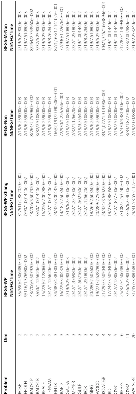
It has been proved that [] problems with initial points are an effective tool to estimate the performance of algorithms and are one of the most commonly used sets of optimization problems. Many scholars use these problems to assess their algorithms (see [, , , ]). In this paper, we also perform experiments on these problems. The detailed numeri-cal results are listed in Table , where the columns of Table have the following meaning:
Problem: the name of the test problem;
Dim: the dimensions of the problem;
NI: the total number of iterations;
Time: the cpu time in seconds;
NFG: NFG=NF+ NG, whereNFandNGare the total number of function and
gra-dient evaluations, respectively (see []).
Ta
b
le
1
(
C
o
ntin
ued
)
Pro
b
le
m
D
im
B
F
G
S
-W
P
NI/NFG/T
ime
BFGS
-W
P
-Zhang
NI/NFG/T
ime
BFGS
-Non
NI/NFG/T
ime
BFGS
-M
-Non
NI/NFG/T
ime
R
O
SEX
100
229/3,704/1.268073e+000
276/4,359/1.512174e+000
2/19/1.126620e–002
2/19/1.251800e–002
SINGX
400
65/922/1.174939e+001
155/2,375/2.844465e+001
2/19/2.065470e–001
2/19/2.115542e–001
PEN1
400
2/47/7.247922e–001
2/47/7.310512e–001
2/19/1.940290e–001
2/19/1.927772e–001
PEN2
200
2/25/6.884900e–002
2/25/6.634540e–002
2/19/6.008640e–002
2/19/6.384180e–002
VA
RDIM
100
2/47/2.879140e–002
2/47/2.879140e–002
2/19/1.001440e–002
2/19/8.762600e–003
TRIG
500
9/138/1.627340e+002
9/144/1.671604e+002
8/146/1.700345e+002
50/876/1.039274e+003
B
V
500
2/19/3.492522e–001
2/19/3.492522e–001
2/19/3.480004e–001
2/19/3.517558e–001
IE
500
6/71/7.711088e+000
6/71/7.706081e+000
6/71/7.722354e+000
6/71/7.772426e+000
TRID
500
53/760/1.622333e+001
50/727/1.501159e+001
564/7,325/1.690631e+002
564/7,325/1.692333e+002
BAND
500
12/275/5.551733e+000
12/238/4.696754e+000
2/19/4.781876e–001
2/19/4.431372e–001
LIN
500
2/19/4.719286e–001
2/19/4.744322e–001
2/19/4.806912e–001
2/19/4.719286e–001
LIN1
500
3/32/9.363464e–001
3/32/9.388500e–001
3/31/9.050514e–001
3/31/9.025478e–001
LIN0
500
3/32/1.165426e+000
3/32/1.161670e+000
3/31/1.119109e+000
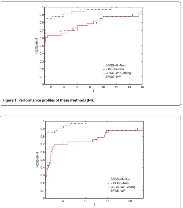
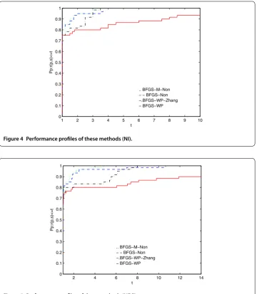
Figure 1 Performance profiles of these methods (NI).
Figure 2 Performance profiles of these methods (NFG).
results in Table indicate that the proposed method is competitive with the other three similar methods.
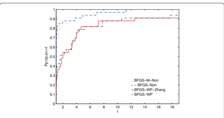
To directly illustrate the performance of these methods, we utilize the tool of Dolan and Moré [] to analyze their efficiency. Figures , , and show that the performance is related toNI,NFG, andTime, respectively. According to these three figures, the MN-BFGS-A method has the best performance (the highest probability of being the optimal solver).
Figure shows that M-Non and Non outperform WP and BFGS-WP-Zhang on approximately %and %of the problems, respectively. The BFGS-WP-Zhang and BFGS-WP methods can successfully solve %and %of the test problems, respectively.
[image:10.595.119.481.80.490.2]BFGS-WP-Figure 3 Performance profiles of these methods (Time).
Zhang and the BFGS-WP methods solve the test problems with probabilities of %and %, respectively.
Figure shows that the success rates when using the BFGS-M-Non and BFGS-Non methods to address the test problems are higher than the success rates when using BFGS-WP and BFGS-BFGS-WP-Zhang by approximately %and %, respectively. Additionally, the BFGS-M-Non and BFGS-Non algorithms can address almost all the test problems. More-over, BFGS-WP-Zhang has better results than BFGS-WP.
5.2 Benchmark problems
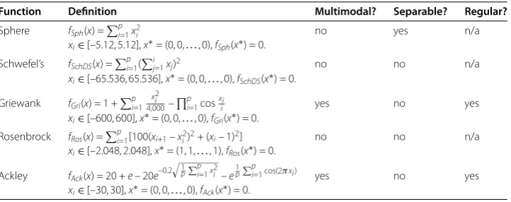
The benchmark problems listed in Table are widely applied in various practical engineer-ing situations. A function is multimodal if it has two or more local optima. A functionp
of the responding variables is separable provided that it can be rewritten as a sum ofp
functions of just one variable []. Separability is closely related to the concept of epista-sis or interrelation among the variables of a function. Non-separable functions are more difficult to optimize because the accuracy of the searching direction depends on two or more variables. By contrast, separable functions can be optimized for each variable in turn. The problem is even more difficult if the function is multimodal. The search process must be able to avoid the regions around local minima in order to approximate, as closely as possible, the global optimum. The most complex case appears when the local optima are randomly distributed in the search space.
The dimensionality of the search space is another important factor in the complexity of the problem. A study of the dimensionality problem and its features was conducted by Friedman []. To establish the same degree of difficulty in all cases, a search space of dimensionalityp= is chosen for all the functions. In the experiment, we do not fix the value top= , namely, it can be larger than . The exact dimensions can be found in Table .
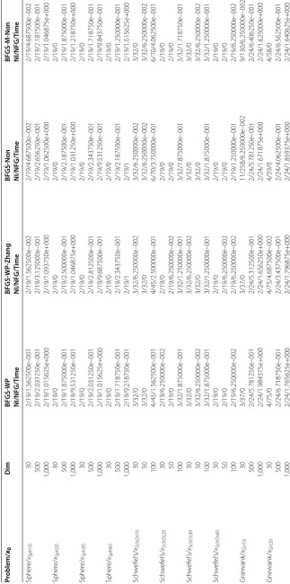
[image:11.595.118.477.78.268.2]Table 2 Definition of the benchmark problems and their features
Function Definition Multimodal? Separable? Regular?
Sphere fSph(x) =pi=1x2
i no yes n/a
xi∈[–5.12, 5.12],x∗= (0, 0,. . ., 0),fSph(x∗) = 0.
Schwefel’s fSchDS(x) =pi=1(ij=1xj)2 no no n/a
xi∈[–65.536, 65.536],x∗= (0, 0,. . ., 0),fSchDS(x∗) = 0.
Griewank fGri(x) = 1 +pi=1 x
2
i
4,000– p
i=1cosxii yes no yes
xi∈[–600, 600],x∗= (0, 0,. . ., 0),fGri(x∗) = 0.
Rosenbrock fRos(x) =pi=1[100(xi+1–xi2)2+ (xi– 1)2] no no n/a xi∈[–2.048, 2.048],x∗= (1, 1,. . ., 1),fRos(x∗) = 0.
Ackley fAck(x) = 20 +e– 20e–0.2
1
p
p
i=1xi2–e1ppi=1cos(2πxi) yes no yes
xi∈[–30, 30],x∗= (0, 0,. . ., 0),fAck(x∗) = 0.
whether an algorithm is better than another algorithm for every function is a fruitless task. Therefore, when an algorithm is evaluated, we identify the types of problems where its performance is good to characterize the types of problems for which the algorithm is suitable. The authors previously studied functions to be optimized to construct a test set with a better selection of fewer functions (see [, ]). This enables us to draw conclu-sions about the performance of the algorithm depending on the type of function.
The above benchmark problems and the discussions of the choice of test problems for an algorithm can be found at
http://www.cs.cmu.edu/afs/cs/project/jair/pub/volume/ortizboyera-html/ node.html.
Many scholars use these problems to test numerical optimization methods (see [, ] etc.). Based on the above discussions, in this subsection, we test the four algorithms on the Benchmark problems. The test results are presented in Table , wherexdenotes the initial point,xSph= (–, –, . . . , –),xSph= (, , . . . , ),xSph= (–, , –, , . . .),xSph= (, , , , . . .),xSchDS= (–., –., . . . , –.),xSchDS= (., ., . . . , .), xSchDS = (–., , –., , . . .), xSchDS = (., , ., , . . .),
xGri = (–, –, . . . , –), xGri = (, , . . . , ), xGri = (–, , –, , . . .), xGri = (, , , , . . .),xRos= (., ., . . . , .),xRos= (., ., . . . , .),xRos= (., , ., , . . .), xRos = (., , ., , . . .), xAck = (–., –., . . . , –.), xAck = (., ., . . . , .),xAck= (–., , –., , . . .), andxAck= (., , ., , . . .).
The numerical results in Table show that the proposed algorithm performs the best among the four methods. The total cpu time of the proposed algorithm is the shortest. BFGS-Non performs better than BFGS-WP and BFGS-WP-Zhang, which is consistent with the results of []. Additionally, BFGS-WP-Zhang performs better than BFGS-WP, which is consistent with the results of []. To directly illustrate the performances of these four methods, we also use the tool of Dolan and Moré [] to analyze the results with respect to NI and NFG in Table . Figures and show their performances.
Figure indicates that BFGS-WP can solve approximately % of the test problems and that the other three methods can solve all the problems. The proposed algorithm solves the problems in the shortest amount of time.
The performance in Figure is similar to that in Figure . BFGS-WP can solve approx-imately % of the test problems, while the other methods can solve all the problems.
Figure 4 Performance profiles of these methods (NI).
Figure 5 Performance profiles of these methods (NFG).
numerical results of the [] and benchmark problems, the GLL nonmonotone line search with Newton update is more effective than the normal WWP line search with quasi-Newton update, which is consistent with the results of [, ]. Moreover, these numerical results indicate that the modified BFGS equation (.) is better than the normal BFGS update, which is consistent with the results of []. Furthermore, the proposed algorithm is competitive with the related methods.
6 Conclusion
(i) This paper conducts a further study of the modified BFGS update formula in []. The main contribution is the global convergence and superlinear convergence for generally convex functions. The numerical results show that the proposed method is competitive with other quasi-Newton methods for the test problems.
[image:15.595.119.480.81.495.2]functions. The conditions of this paper are weaker than those of the previous research.
(iii) For further research, we should study the performance of the new algorithm under different stop rules and in different testing environments (such as []). Moreover, more numerical experiments for large practical problems should be performed in the future.
Acknowledgements
The authors thank the referees for their valuable comments, which greatly improved their paper.
Funding
This work is supported by the China NSF (Grant No. 11261006 and 11661009), the Guangxi Science Fund for
Distinguished Young Scholars (No. 2015GXNSFGA139001),and the basic ability promotion project of Guangxi young and middle-aged teachers (No. 2017KY0019).
Competing interests
The authors declare that they have no competing interests.
Authors’ contributions
Mr. XL wrote and organized the paper. Dr. BW performed the algorithm experiments and wrote the code. Dr. WH studied the BFGS-type methods. Only the authors contributed to writing this paper. All authors read and approved the final manuscript.
Publisher’s Note
Springer Nature remains neutral with regard to jurisdictional claims in published maps and institutional affiliations.
Received: 20 March 2017 Accepted: 14 July 2017 References
1. Fu, Z, Wu, X, Guan, C, et al.: Toward efficient multi-keyword fuzzy search over encrypted outsourced data with accuracy improvement. IEEE Trans. Inf. Forensics Secur.11(12), 2706-2716 (2016)
2. Gu, B, Sheng, VS, Tay, KY, et al.: Incremental support vector learning for ordinal regression. IEEE Trans. Neural Netw. Learn. Syst.26(7), 1403-1416 (2015)
3. Gu, B, Sun, X, Sheng, VS: Structural minimax probability machine. IEEE Trans. Neural Netw. Learn. Syst.99, 1-11 (2016) 4. Li, J, Li, X, Yang, B, et al.: Segmentation-based image copy-move forgery detection scheme. IEEE Trans. Inf. Forensics
Secur.10(3), 507-518 (2015)
5. Pan, Z, Zhang, Y, Kwong, S: Efficient motion and disparity estimation optimization for low complexity multiview video coding. IEEE Trans. Broadcast.61(2), 166-176 (2015)
6. Pan, Z, Lei, J, Zhang, Y, et al.: Fast motion estimation based on content property for low-complexity H.265/HEVC Encoder. IEEE Trans. Broadcast.99, 1-10 (2016)
7. Yuan, G, Lu, S, Wei, Z: A new trust-region method with line search for solving symmetric nonlinear equations. Int. J. Comput. Math.88(10), 2109-2123 (2011)
8. Yuan, G, Meng, Z, Li, Y: A modified Hestenes and Stiefel conjugate gradient algorithm for large-scale nonsmooth minimizations and nonlinear equations. J. Optim. Theory Appl.168(1), 129-152 (2016)
9. Yuan, G, Wei, Z: The Barzilai and Borwein gradient method with nonmonotone line search for nonsmooth convex optimization problems. Math. Model. Anal.17(2), 203-216 (2012)
10. Yuan, G, Wei, Z, Li, G: A modified Polak-Ribière-Polyak conjugate gradient algorithm for nonsmooth convex programs. J. Comput. Appl. Math.255, 86-96 (2014)
11. Yuan, G, Wei, Z, Lu, S: Limited memory BFGS method with backtracking for symmetric nonlinear equations. Math. Comput. Model.54(1-2), 367-377 (2011)
12. Yuan, G, Wei, Z, Lu, X: A BFGS trust-region method for nonlinear equations. Computing92(4), 317-333 (2011) 13. Yuan, G, Wei, Z, Wang, Z: Gradient trust region algorithm with limited memory BFGS update for nonsmooth convex
minimization. Comput. Optim. Appl.54(1), 45-64 (2013)
14. Yuan, G, Yao, S: A BFGS algorithm for solving symmetric nonlinear equations. Optimization62(1), 85-99 (2013) 15. Yuan, G, Zhang, M: A three-terms Polak-Ribière-Polyak conjugate gradient algorithm for large-scale nonlinear
equations. J. Comput. Appl. Math.286, 186-195 (2015)
16. Yuan, G, Zhang, M: A modified Hestenes-Stiefel conjugate gradient algorithm for large-scale optimization. Numer. Funct. Anal. Optim.34(8), 914-937 (2013)
17. Schropp, J: A note on minimization problems and multistep methods. Numer. Math.78(1), 87-101 (1997) 18. Schropp, J: One-step and multistep procedures for constrained minimization problems. IMA J. Numer. Anal.20(1),
135-152 (2000)
19. Wyk, DV: Differential optimization techniques. Appl. Math. Model.8(6), 419-424 (1984)
20. Vrahatis, MN, Androulakis, GS, Lambrinos, JN, et al.: A class of gradient unconstrained minimization algorithms with adaptive stepsize. J. Comput. Appl. Math.114(2), 367-386 (2000)
22. Yuan, G, Duan, X, Liu, W, et al.: Two new PRP conjugate gradient algorithms for minimization optimization models. PLoS ONE10(10), e0140071 (2015)
23. Yuan, G, Wei, Z: New line search methods for unconstrained optimization. J. Korean Stat. Soc.38(1), 29-39 (2009) 24. Yuan, G, Wei, Z: A trust region algorithm with conjugate gradient technique for optimization problems. Numer. Funct.
Anal. Optim.32(2), 212-232 (2011)
25. Yuan, G, Wei, Z, Zhao, Q: A modified Polak-Ribière-Polyak conjugate gradient algorithm for large-scale optimization problems. IIE Trans.46(4), 397-413 (2014)
26. Broyden, C: The convergence of a class of double rank minimization algorithms. J. Inst. Math. Appl.6(1), 222-231 (1970)
27. Fletcher, R: A new approach to variable metric algorithms. Comput. J.13(2), 317-322 (1970)
28. Goldfarb, A: A family of variable metric methods derived by variational means. Math. Comput.24(109), 23-26 (1970) 29. Schanno, J: Conditions of quasi-Newton methods for function minimization. Math. Comput.24(4), 647-650 (1970) 30. Broyden, CG, Dennis, JE, Moré, JJ: On the local and superlinear convergence of quasi-Newton methods. J. Inst. Math.
Appl.12(3), 223-245 (1973)
31. Byrd, RH, Nocedal, J: A tool for the analysis of quasi-Newton methods with application to unconstrained minimization. SIAM J. Sci. Comput.26(3), 727-739 (1989)
32. Byrd, RH: Global convergence of a cass of quasi-Newton methods on convex problems. SIAM J. Numer. Anal.24(5), 1171-1190 (1987)
33. Dennis, JE: Quasi-Newton methods, motivation and theory. SIAM Rev.19(1), 46-89 (1977)
34. Dennis, JE: A characterization of superlinear convergence and its application to quasi-Newton methods. Math. Comput.28(126), 549-560 (1974)
35. Dai, YH: Convergence properties of the BFGS algoritm. SIAM J. Optim.13(3), 693-701 (2002)
36. Mascarenhas, WF: The BFGS method with exact line searches fails for non-convex objective functions. Math. Program. 99(1), 49-61 (2004)
37. Li, DH, Fukushima, M: A modified BFGS method and its global convergence in nonconvex minimization. J. Comput. Appl. Math.129(1-2), 15-35 (2001)
38. Li, DH, Fukushima, M: On the global convergence of BFGS method for nonconvex unconstrained optimization problems. SIAM J. Optim.11(4), 1054-1064 (1999)
39. Wei, Z, Yu, G, Yuan, G, et al.: The superlinear convergence of a modified BFGS-type method for unconstrained optimization. Comput. Optim. Appl.29(3), 315-332 (2004)
40. Wei, Z, Li, G, Qi, L: New quasi-Newton methods for unconstrained optimization problems. Appl. Math. Comput. 175(2), 1156-1188 (2006)
41. Yuan, G, Wei, Z: Convergence analysis of a modified BFGS method on convex minimizations. Comput. Optim. Appl. 47(2), 237-255 (2010)
42. Zhang, JZ, Deng, NY, Chen, LH: New quasi-Newton equation and related methods for unconstrained optimization. J. Optim. Theory Appl.102(1), 147-167 (1999)
43. Yuan, G, Wei, Z, Wu, Y: Modified limited memory BFGS method with nonmonotone line search for unconstrained optimization. J. Korean Math. Soc.47(4), 767-788 (2010)
44. Davidon, WC: Variable metric method for minimization. SIAM J. Optim.1(1), 1-17 (1991)
45. Powell, MJD: A new algorithm for unconstrained optimization. In: Nonlinear Programming, pp. 31-65. Academic Press, New York (1970)
46. Yuan, G, Wei, Z, Lu, X: Global convergence of BFGS and PRP methods under a modified weak Wolfe-Powell line search. Appl. Math. Model.47, 811-825 (2017)
47. Grippo, L, Lampariello, F, Lucidi, S: A nonmonotone line search technique for Newton’s method. SIAM J. Sci. Comput. 23(4), 707-716 (1986)
48. Grippo, L, Lampariello, F, Lucidi, S: A truncated Newton method with nonmonotone line search for unconstrained optimization. J. Optim. Theory Appl.60(3), 401-419 (1989)
49. Grippo, L, Lampariello, F, Lucidi, S: A class of nonmonotone stabilization methods in unconstrained optimization. Numer. Math.59(1), 779-805 (1991)
50. Liu, G, Han, J, Sun, D: Global convergence of the BFGS algorithm with nonmonotone linesearch. Optimization34(2), 147-159 (1995)
51. Han, J, Liu, G: Global convergence analysis of a new nonmonotone BFGS algorithm on convex objective functions. Comput. Optim. Appl.7(3), 277-289 (1997)
52. Yuan, GL, Wei, ZX: The superlinear convergence analysis of a nonmonotone BFGS algorithm on convex objective functions. Acta Math. Sin. Engl. Ser.24(1), 35-42 (2008)
53. Raydan, M: The Barzilai and Borwein gradient method for the large scale unconstrained minimization problem. SIAM J. Sci. Comput.7(1), 26-33 (1997)
54. Toint, PL: An assessment of nonmonotone linesearch techniques for unconstrained optimization. SIAM J. Sci. Comput.17(3), 725-739 (2012)
55. Zhang, H, Hager, WW: A nonmonotone line search technique and its application to unconstrained optimization. SIAM J. Optim.14(4), 1043-1056 (2006)
56. Powell, MJD: Some properties of the variable metric algorithm. In: Numerical Methods for Non-linear Optimization, pp. 1-17. Academic Press, London (1972)
57. Moré, JJ, Garbow, BS, Hillstrom, KE: Testing unconstrained optimization software. ACM Trans. Math. Softw.7(1), 17-41 (1981)
58. Dolan, ED, Moré, JJ: Benchmarking optimization software with performance profiles. Math. Program.91(2), 201-213 (2002)
59. Hadley, G: Nonlinear and Dynamics Programming. Addison-Wesley, New Jersey (1964)
60. Friedman, JH: An overview of predictive learning and function approximation. In: Cherkassky, V, Friedman, JH, Wechsler, H (eds.) From Statistics to Neural Networks, Theory and Pattern Recognition Applications. NATO ASI Series F, vol. 136, pp. 1-61. Springer, Berlin (1994)
62. Salomon, R: Reevaluating genetic algorithm performance under coordinate rotation of benchmark functions. Biosystems39(3), 263-278 (1996)
63. Whitley, D, Mathias, K, Rana, S, Dzubera, J: Building better test functions. In: Eshelman, L (ed.) Sixth International Conference on Genetic Algorithms, pp. 239-246. Kaufmann, California (1995)
64. Yuan, G, Lu, X, Wei, Z: A conjugate gradient method with descent direction for unconstrained optimization. J. Comput. Appl. Math.233(2), 519-530 (2009)
65. Yuan, G, Lu, X, Wei, Z: BFGS trust-region method for symmetric nonlinear equations. Biosystems230(1), 44-58 (2009) 66. Gould, NIM, Orban, D, Toint, PL: CUTEr and SifDec: a constrained and unconstrained testing environment, revisited.