Performances Assessment of MOMA-Plus Method on Multiobjective Optimization Problems

(1)

Vol. 13, No. 1, 2020, 48-68

ISSN 1307-5543 – www.ejpam.com Published by New York Business Global

Performances assessment of MOMA-Plus method on

multiobjective optimization problems

Alexandre Som1_{, Kounhinir Som´}_e2∗_{, Abdoulaye Compaor´}_e2_{, Blaise Som´}_e1 1 _{Department of Mathematics, Laboratory of Numerical Analysis, Computer Science and}

Biomathematics, Joseph Ki-Zerbo University, Ouagadougou, Burkina Faso.

2 _{Department of Mathematics, Laboratory of Fundamental and Applied Mathematics,}

Nor-bert Zongo University, Koudougou, Burkina Faso.

Abstract. This work is devoted to evaluate the performances of the MOMA-Plus method in solving multiobjective optimization problems. This assessment is doing on the complexity of its algorithm, the convergence and the diversity of solutions in relation to the Pareto front. All these parameters were evaluated on non-linear multiobjective test problems and obtained solutions are compared with those provided by the NSGA-II method. This comparative study made it possible to highlight the performances of MOMA-Plus method for solving non-linear multiobjective problems.

2020 Mathematics Subject Classifications: 90C29, 90C30, 49M30, 49M37

Key Words and Phrases: Multiobjective optimization, MOMA-Plus method, Performances assessment

1. Introduction

Multi-objective optimization has been, for several decades, a discipline of Mathe-matics that allows to solve optimization problems where several criteria are involved simultaneously[1, 9, 13, 14]. Several researchers have developed methods or algorithms to find compromise solutions which would be as close as possible to the best values of criteria but also verify the constraints. Most of these methods can be classified in two groups: the exact methods and metaheuristics. Metaheuristics have been developed to overcome the shortcomings of direct or traditional methods. Indeed, on some kinds of problems, direct or traditional methods are unable either to find Pareto optimal solutions, or to converge quickly towards the Pareto front, or to give a good distribution of solu-tions around the Pareto front. Therefore, metaheuristics are developed to overcome these shortcomings.

In literature, we can find several metaheuristics among which the best known and the

∗

Corresponding author.

DOI: https://doi.org/10.29020/nybg.ejpam.v13i1.3581

Email addresses: [email protected](A. Som),[email protected](K. Somé), [email protected](A. Compaoré),[email protected](B. Somé)

(2)

most used are: simulated annealing[10], tabu search[11], genetic algorithms[9], NSGA-II algorithm[1], MOMA method[15, 19, 22], MOMA-Plus method[23], and more.

In this article, we will focus on the MOMA-Plus method. Indeed, MOMA (Multi-Objective Metaheuristic based on Alienor method) have been developed by K. Som´e et al.[15, 22] and is based on an Alienor transformation[4]. It uses scalarization and penal-ization techniques to transform the multiobjective problem with constraints into a single objective problems without constraints and with only one variable. It has provided sat-isfying results[15, 19, 22] and even it has been improved. This improvement has given rise to the MOMA-Plus method[23]. The MOMA-Plus method uses the Nelder-Mead[16] algorithm instead of Operator Preserving Optimality (OPO) to find the optimum in a discretized domain. The idea of associating the Nelder-Mead algorithm is the fact that there is a dependence on the choice of an parameter θ0 in using the OPO [19, 23] in the MOMA algorithm that influences MOMA efficiency.

Note that the MOMA-Plus method has been designed to solve deterministic multi-objective continuous variable optimization problems. But later, some authors adapted it to solve other types of optimization problems. We can quote: A. Compaor´e et al[17, 20] for fuzzy optimization problems, and J. Poda et al[7, 8] for combinatorial optimization problems. However, a study of performances of the MOMA-Plus method has not been done yet, hence the purpose of this work.

Indeed, in this article, we intend to evaluate the performance of the MOMA-Plus method on some test problems. For this purpose, a comparative study of the obtained results will be done on these test problems using the NSGA-II method developed by K. Deb et al[1]. Therefore, we provide a complete study on the performances of the MOMA-Plus method because in all of the former works on MOMA-MOMA-Plus, no study has been done about the complexity of the algorithm, the convergence and the diversity of solutions on the Pareto front.

(3)

2. MOMA-Plus method

Let’s consider n, m and p be natural integers. Let’s consider also the following multi-objective optimization problem:

minf(x) =

f1(x),· · · , fp(x)

T

s.t:

(

g(x) =

g1(x),· · ·, gm(x)

T

≤0; x = (x1,· · ·, xn)∈Rn;

(1)

where fj, j = 1, p are the objective functions, gi, i = 1, m are the constraints of the

problem and x= (x1,· · ·, xn) are the decision variables.

Some definitions are necessary for the best understanding of this work. LetS be the set of eligible solutions, i.e. S={x∈_Rn_/g

1(x)≤0;...;gm(x)≤0}.

Definition 1. A solution x∗ ∈ S is called Pareto optimal if there is no other solution x ∈ S such that fj(x) ≤ fj(x∗),∀j ∈ {1, .., p} and for a certain k ∈ {1, .., p} such that fk(x)< fk(x∗).

Definition 2. The ideal point is the vector z ∈ _Rp _{whose components} _z

j are obtained by

individually minimizing each objective function fj, under on all constraints. We have:

zj = minfj(x) s.t:

g(x) = (g1(x),· · · , gm(x))T ≤0; x= (x1,· · ·, xn)∈Rn.

(2)

The steps of the MOMA-Plus method are as follow: (i) aggregation of objective functions;

(ii) penalization constraints; (iii) reduction of research space;

(iv) resolution in the reduced search space

(v) configuration of the solution to the initial space.

2.1. Aggregation of objective functions

The MOMA-Plus method uses an aggregation technique to transform the multiobjec-tive optimization problem into a single-objecmultiobjec-tive optimization problem. The aggregation function used here is the weighted Tchebychev distance because all problems are non-linear. It is defined by the following equation:

H(f(x), λ, z) = max

(4)

The coefficientsλk,k= 1, pare weights of the objective functions with p

X

k=1

λk = 1.

By applying (3) to the problem (1) we obtain: min H(f(x), λ, z) s.t:

g(x) = (g1(x),· · · , gm(x))T ≤0; x= (x1,· · ·, xn)∈Rn.

(4)

The problem (4) is mono-objective, therefore it can have a global optimum for a fixed λ. The following theorems prove the equivalence between the solutions of the initial problem and the aggregate problem.

Theorem 1. Any Pareto optimal solution of the problem (1) is an optimal solution for the problem (4) and reciprocally.

Proof. Let x∗ be an Pareto optimal solution of the problem (1) and note that I =

{1,2,· · · , p}. Then, there is nox∈S such as :

fj(x)≤fj(x∗),∀j∈I and k6=j such asfj(x)< fj(x∗).

Let’s suppose thatx∗ is not an optimal solution for the problem (4). Then :

∃x∈S :H(f(x), λ, z)< H(f(x∗), λ, z).

That is equivalent to

∃x∈S: max

j∈I

λj|fj(x)−zj| ≤max j∈I

⇒ ∃x∈S,∃l∈I :|fl(x)−zl| ≤ |fl(x∗)−zl|, because λ≥0

⇒ ∃x∈S,∃l∈I :fl(x)−zl≤fl(x∗)−zl, because (fl(x)−zl≥0,∀x∈S) ⇒ ∃x∈S,∃l∈I :fl(x)≤fl(x∗) that is absurd

Consequently, x∗ is an optimal solution of problem (4). Now, let x∗ be an optimal solution of problem (4). Then

∀x∈S :H(f(x∗), λ, z)< H(f(x), λ, z).

Let’s suppose thatx∗ is not an Pareto optimal solution for the problem (1). Then :

∃x∈S,∀j∈I, fj(x)< fj(x∗)

⇒ ∃x∈S,∀j∈I, fj(x)−zj < fj(x∗)−zj

⇒ ∃x∈S,∀j∈I, λj|fj(x)−zj|< λj|fj(x∗)−zj| ⇒ ∃x∈S,∀j∈I,max

j∈I

λj|fj(x)−zj| <max j∈I

λj|fj(x∗)−zj| ⇒ ∃x:H(f(x), λ, z)< H(f(x∗), λ, z), that is absurd.

(5)

2.2. Penalization

This step consists in transforming the problem (4) into an optimization problem with-out constraints. The used penalty function derives from the Lagrangian function and is defined by[21]:

L(x) =H(f(x), λ, z) +η m

X

i=1

(gi(x) +|gi(x)|). (5)

η is the defined penalty coefficient such as :

η ≥ M−H_X(f(x), λ, z)

i=1,m gi

withM = max

x∈S H(f(x), λ, z)

.

By using the function (5), the problem (4) becomes a single objective optimization problem without constraint given by the following formulation:

(

Glob.minL(x)

x∈D; (6)

withD, a subset ofRndefined by the boundaries of the variables. The following theorem characterizes the global optimum of the problem (6).

Theorem 2. Let x∗ ∈ S be a point that realizes the global minimum of the problem (6) thenx∗ is a point that realizes global minimum of the problem (4).

Proof. Let’s suppose thatx∗ is a point that realizes the global minimum of the problem (6) then ∀x∈S :L(x∗)≤L(x) that means that:

∀x∈S, L(x∗)≤L(x),

then

H(f(x∗), λ, z) +η m

X

k=1

(gk(x∗) +|gk(x∗)|)< H(f(x), λ, z) +η m

X

k=1

(gk(x) +|gk(x)|).

By the definition of the setS we have gi(x)≤0⇒gi(x) +|gi(x)|= 0 therefore we have: m

X

i=1

gi(x) +|gi(x)|

= 0

Consequently,

H(f(x∗), λ, z)≤H(f(x), λ, z)

(6)

2.3. Reduction of research space

Definition 3. The Alienor transformation is any transformation that reduces a function of several variables to a function of a single variable using the α−dense curves which corresponds to a reduction of the search space.

Theα−dense curves are studied in [6] and the interested reader will be able to consult it. The Alienor transformation that we will use in this work is that of Konf´e-Cherruault[4]. It is given by the following equation:

xi=hi(θ) =

1 2

(bi−ai) cos(ωiθ+φi) +ai+bi

, i= 1,· · · , n. (7)

In the equation (7), ωi and φi are slowly increasing sequences and θ ∈ [0;θmax] with θmax=

(b−a)θ1+ (b+a)

2 and θ

1 ₌ 2π−φ1 ω1

.

Several types of Alienor transformations exist in the literature and the interested read-ers will be able to consult [2, 3, 5, 6, 12].

By applying the equation (7) to the variables of the problem (6), we obtain the opti-mization problem with single objective without constraint and with only one variable by the following formulation:

(

Glob.min F(θ) θ∈[0;θmax].

(8)

Theorem 3. Any minimum of the problem (6) can be approached by a minimum of the problem (8).

Proof. For the proof, see [5].

The resolution of the problem (8) is to find the θvalue that minimizes the functionF.

2.4. Resolution in reduced space

The MOMA-Plus method is applied in a discrete interval to which the Nelder-Mead algorithm is applied, more precisely in the neighborhood of the discrete points, as shown in the following figure :

(7)

This process is repeated until the coverage of the whole domain. Nelder-Mead’s method known as fminsearch in Matlab, is very effective for optimization of a single variable[16]. To maximize the chances of obtaining the global optimum, the research domain has been discretized in nested domains with centerxi and the search for a local solution is realized

next to neighborhood of each point. It is among these solutions that the overall optimum will be chosen.

2.5. Configuration of the obtained solutions to the initial space

After the execution of Nelder-Mead’s algorithm, the last step of MOMA-Plus is the configuration of the obtained solutions. Indeed, it is the transition from the optimal θto the variablesxiusing in the formulation (7). Note that this solution configuration provides

all the Pareto optimal solutions for the initial problem.

2.6. MOMA-Plus algorithm

The algorithm of the MOMA-Plus method is as follows : Algorithm 1 Algorithm of the MOMA-Plus method

(i) For k from 1 top do

f(x)←−maxλk|fk(x)−zk|(”scalarization”)

End For

(ii) g(x)←−g1(x) +|g1(x)|

Forifrom 2 to m do g(x)←−gi(x) +|gi(x)|

End For

L(x)←−f(x) +η∗g(x)(”Penalization”) (iii) For ifrom 1 to ndo (”Space reduction”)

xi =hi(θ)

End For

f(θ)←−f(h1(θ), h2(θ),· · · , hn(θ))

(iv) θ←−N elder−M ead(F(θ)) (”Resolution in reducing space”) (v) For iFrom 1 to n, (Configuration)

xi =hi(θ) (”Solutions configuration”)

End for

(8)

3. Performances analysis

Performances analysis is done on the test problems defined below. This analysis is mainly based on the complexity of computation time, convergence and diversity.

3.1. Complexity study

The MOMA-Plus algorithm starts with the scalarization where it is about a compar-ison of p quantity λk(fk−zk), of which the complexity at worst is O(p2). Then, follows

the penalization, at this level the complexity is O(m) at worst with m the number of constraints. The complexity of the transformation of decision variables into a single vari-able is at worst equal to O(n). Let J + 1 be the size of formed simplex for applying the Nelder-Mead algorithm where J is the size of search space. In our work, the search space is one dimension so J = 1. Therefore, the complexity of Nelder-Mead algorithm in MOMA-Plus method is constant. Then, as the search space is discretized into N + 1 points the complexity of Nelder-Mead isO(N). After finding the optimum by the Nelder-Mead algorithm, the next step is to reconstruct the global and final solution. This step is complex. So in one iteration, the complexity is:

O(p2) +O(m) +O(n) +O(N) +O(n).

If the size of the weight coefficients is K then the final complexity of the MOMA-Plus algorithm is :

T =K.O(max{p2;m;n;N2}). (9) This result is justified by the bellow theorem:

Theorem 4. Let f andg be two functions of the variable n∈_Nand with positive values. Let’s consider two algorithms A and B of complexity respectively O(f(n)) and O(g(n)). We have:

O(f(n)) +O(g(n)) =O(f(n) +g(n)) =O(max{f(n);g(n)}). Proof. For the demonstration, see [18]

The other method that we present in this work, and whose results will be compared. With those of the MOMA-Plus method, is the NSGA-II method (Non-dominated Sorted Genetic Algorithm II). It was developed by Deb and Srinivas[1]. It is a method that uses the concept of elitism for which the best solutions are preserved and used through the notion of Pareto dominance the distance of obstruction-[1] the crossover and mutation op-erations for the creation of next generation. That makes the algorithm quickly convergence towards the optimal solutions.

The complexity of the NSGA-II method is O(p.n2)[1]; where p is the size of the used objective functions and nis the size of the input variables.

(9)

3.2. Test problems and numerical experiments

The problems below have been solved by K. Deb in [1], where he is doing a comparative study between the NSGA-II and some algorithms like SPEA†, PAES‡, etc. The result of this study was that the NSGA-II method provided satisfactory results compared to the other methods.

In this work, we propose a comparative study of performances through the convergence and diversity metrics of the MOMA-Plus and NSGA-II methods. The problems we have used are recorded in the table below :

Table 1: multiobjective problems

Min-Ex: SCH:

          

minf1(x1, x2) =x1

minf2(x1, x2) =

1 +x2

x1

0.16x161

06x265



 

 

minf1(x) =x2

minf2(x) = (x−2)2

−56x65

PLN1: PLN2:               

minf1(x) =x1

minf2(x) =g(x)×

1−(f1(x)

g(x))

2

g(x) = 1 + 9

n−1×

n

P

i=2

xi

x= (x1, x2, ..., xn)∈[0.1]n

                      

minf1(x) =x1

minf2(x) =g(x)×h(x)

g(x) = 1 + 9

n−1×

n

P

i=2

xi

h(x) = 1−

s

f1(x)

g(x) −

f1(x)

g(x) ×sin(10πf1(x))

x= (x1, x2, ..., xn)∈[0.1]n

PLN3: PLN4:                 

minf1(x) =x1

minf2(x) =g(x)× 1− s

f1(x)

g

!

g(x) = 1 + 9

n−1×

n

P

i=2

xi

x= (x1, x2, ..., xn)∈[0.1]n

              

minf1(x) =x1

minf2(x) =g

1−qf1(x)

g

avec g(x) = 1 + 10 (n−1) +

n

P

i=1

(xi−10cos(4πxi))

xi∈[0; 1]

POL: VNT:                       

minf1(x) = 1 + (A1−B1)2+ (A2−B2)2

minf2(x) = (x1+ 3)2+ (x2+ 1)2

A1= 0,5sin(1)−2cos(1) +sin(2)−1,5cos(2)

A2= 1,5sin(1)−cos(1) + 2sin(2)−0,5cos(2)

B1= 0,5sin(x1)−2cos(x1) +sin(x2)−1,5cos(x2)

B2= 1,5sin(x1)−cos(x1) + 2sin(x2)−0,5cos(x2)

x1, x2∈[−π;π]

              

minf1(x) = 0.5(x21+x22) +sin(x21+x22)

minf2(x) =

3x12x2+ 4

8 +

(x1−x2+ 1)2

27 + 15 minf3(x) =

1

x2

1+x22+ 1

−1,1exp(−(x2 1+x22))

x1, x2∈[−3; 3]

KUR:           

minf1(x) = 2 P

i=1

[−10exp(−0.2qx2

i+x2i+1)]

minf2(x) = 3 P

i=1

[|xi|0.8_{+ 5}_sin₍_x3

i)] xi∈[−5; 5], i= 1,2,3

†

Pareto Archived Evolution Strategy

‡

(10)

Note that the domain of the decision variables of the multi-modal problem (PNL4) has changed in comparing to the initial search space.

3.3. Graphical results MOMA-Plus/NSGA-II

In this section we present the results of the simulations of the multiobjective problems. These simulations are made up of Pareto’s analytical front, the different fronts resulting from MOMA-Plus and NSGA-II methods. For the simulations, we used MATLAB R2013b as simulation and programming software.

Remark 1. For the MOMA-Plus method, the parameters are P= size of the objective functions, n= size of the input variables, m= number of constraints, N= size of the dis-cretization.

For the NSGA-II method we will note: GEN=number of generations, POP=population size, PF= Pareto fraction, MUT=type of mutation, CRS=type of crossing, ST-GEN= Stall Generation, the crossing parameter that has been used for these problems is ” crossover-scattered ”.

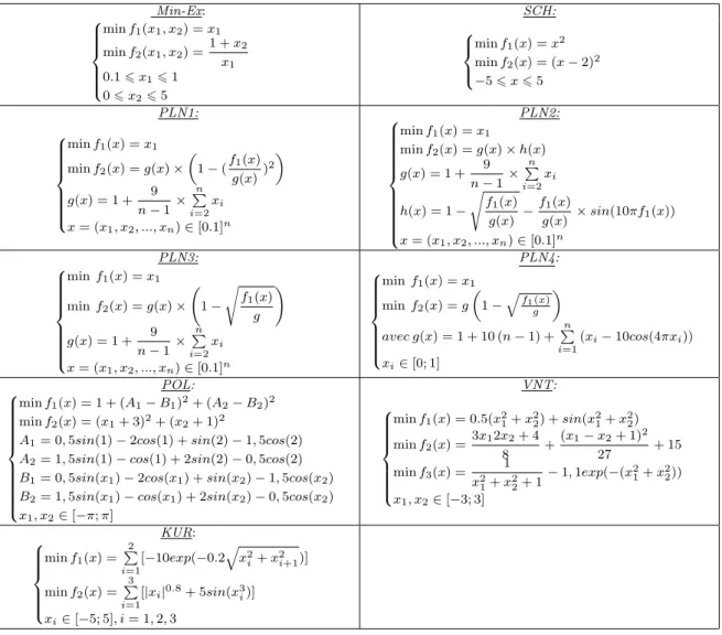
3.3.1. MIN-EX Problem

The resolution parameters of MIN-EX problem are:

• for the NSGA-II method:

Table 2: Parameters for NSGA-II

GEN POP PF MUT ST-GEN Crossover

NSGA-II 250 250 0,5 uniform 300 Scattered

• for the MOMA-Plus method:

Table 3: Parameters for MOMA-Plus

p n m N

MOMA-Plus 2 2 0 100

(11)

Figure 2: MOMA-Plus Pareto front

Figure 3: NSGA-II Pareto Front

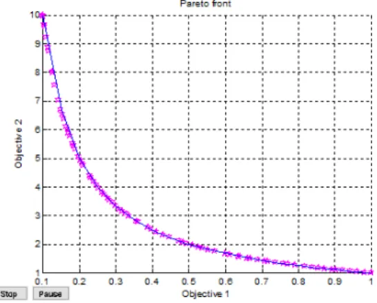
3.3.2. SCH problem

The resolution parameters of SCH problem are:

Table 4: Parameters for NSGA-II method

NSGA-II d´efaut 100 0,5 uniform 300 Scattered

Table 5: Parameters for MOMA-plus method

p n m N

MOMA-Plus 2 2 0 100

(12)

Figure 4: MOMA-Plus Pareto Front

3.3.3. PLN1 problem

The resolution parameters of PLN1 problem are:

• for the NSGA-II method :

Table 6: Parameters for NSGA-II method

p n m N

MOMA-Plus 2 30 0 100

(13)

Figure 6: MOMA-Plus Pareto Front Figure 7: NSGA-II Pareto Front

3.3.4. PLN2 problem

Table 8: Parameters for MOMA-Plus method

p n m N

• for NSGA-II parameters:

(14)

Figure 9: NSGA-II Pareto front

3.3.5. PLN3 problem

p n m N

(15)

Figure 11: NSGA-II Pareto front

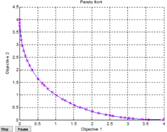
3.4. PLN4 problem

The resolution parameters of PLN4 problem are

• for MOMA-Plus method:

p n m N

• for NSGA-II method:

(16)

Figure 12: MOMA-Plus Pareto Front

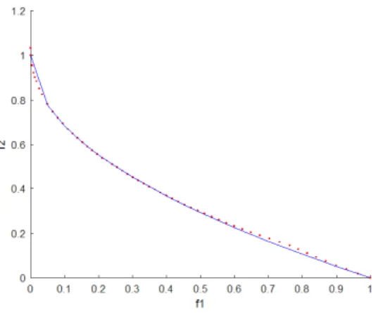
Remark 2. The problems that we have solved until here admit continuous optimal analytic Pareto fronts. So, we have represented in same figure the analytic Pareto front and this is provided by MOMA-Plus or NSGA-II method. That will be not possible for the following problems.

3.4.1. POL Problem

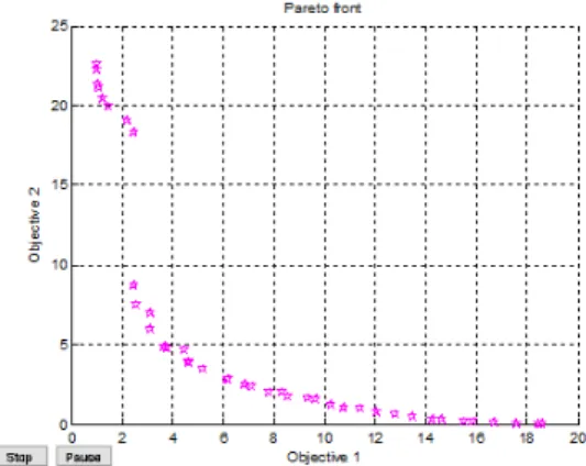
The set of Pareto optimal solution of POL problem is not continuous. Therefore, there is not an analytic front for it. So, we can not represent the two fronts in the same figure. However, we will represent only the obtained fronts from MOMA-plus and NSGA-II.

The resolution parameters of POL problem are:

• for MOMA-Plus method:

p n m N

MOMA-Plus 2 2 0 100

• for NSGA-II method:

(17)

• The fronts are represented below:

Figure 14: Front Pareto MOMA-Plus

Figure 15: Front Pareto NSGA-II

4. Calculation of performance indicators

4.1. Calculation of numerical execution time

In this section we present the time taken by the computer to execute the programs in oder to find the optimal solutions. The characteristic of the used computer are:

• Mark: DELL;

• Processor: INTEL(R) Core(TM) i5-3340M CPU @2.70GHZ 2.70GHZ;

• RAM: 8 GO

• System: 64 bits

the obtained results of the calculation time, in seconds, are recorded in the following table:

Table 16: Numerical calculation time table

MIN-EX SCH PLN1 PLN2 PLN3 PLN4

MOMA-Plus 24,353167 17,875150 115,167287 161,009449 95,343133 127,083839 NSGA-II 9,121357 3,804150 16,211981 11.027945 5,351849 27,864951

We find that NSGA-II is faster than MOMA-Plus.

4.2. Study of the convergence metric

The convergence metric we use here is defined by the following formula[9]:

γ = s

N

P

i=1 d2

i

(18)

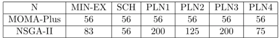
In this metricN is the size of the obtained solution by using MOMA-Plus or NSGA-II solutions. The below table gives the value of N for each method on each problem. di is

the Euclidean distance between the obtained solutioniand that of the nearest analytical front.

Table 17: Size of the solutions obtained

N MIN-EX SCH PLN1 PLN2 PLN3 PLN4

MOMA-Plus 56 56 56 56 56 56

NSGA-II 83 56 200 125 200 75

This metric corresponds to the performance of the method, especially its ability to converge towards the Pareto optimal analytical front. Thus, a high-performance and effective method is one whose γ value is closed to zero. However, the calculation of this metric involves two respective fronts: the given front by the used method and the Pareto optimal analytical front.

The obtained results of the calculation of the convergence metric are recorded in the table below :

Table 18: Metricγ values

γ MIN-EX SCH PLN1 PLN2 PLN3 PLN4

MOMA-Plus 0,0691 0,0053 0,0042 0,0599 0,0137 0,1154 NSGA-II 0,0321 0,0056 0,0025 0,0124 0,0175 0,0274

With regard to these obtained results, we notice that the values of the convergence metric provided by the two methods are all closed to zero. It would mean that the MOMA-Plus method is effective. In addition, we can see that the MOMA-MOMA-Plus method approaches Pareto optimal solutions are better than the NSGA-II method on problems (SCH) and (PLN3).

4.3. Study of the diversity metric

The metric of diversity that we use here is defined by the following formula[9] :

∆ =

M

P

m=1 de_m+

N−1 P

i=1

|di−d|

M

P

m=1 de

m+ (N −1)d

(11)

In the relationship: diis the Euclidean distance between two solutions closed to the Pareto

(19)

front.

The metric of diversity corresponds to the distribution of solutions on the Pareto front. Note that a good distribution is the one whose ∆ value is closed to zero or even equal to zero. The calculation of the metric of diversity of the MOMA-Plus and NSGA-II method are recorded in the following table :

Table 19: Metric∆values

∆ MIN-EX SCH PLN1 PLN2 PLN3 PLN4

MOMA-Plus 1,1833 0,5537 0,0309 0,9818 0,3498 0,9835 NSGA-II 0,0290 0,0183 0,0319 0,0293 1,0023 0,9710

Here, we also see that MOMA-Plus method is better than NSGA-II method on prob-lems (PLN1) and (PNL3.)

4.4. Particular Cases

The problems POL, VNT and KUR are discontinuous fronts and we have not an analytic Pareto front. This makes it difficult to study convergence and diversity. Therefore, a possible comparative study is difficult. Nevertheless, a study of convergence and diversity has been done by combining the two fronts given by MOMA-Plus and NSGA-II that is given us by the below table:

Table 20: joint table of performances

POL VNT KUR

γ 0,7645 0,2429 0,3699 ∆ 0,7341 0.7856 0,7973

With regard to the obtained results, we can see that the solutions provided by the MOMA-Plus and NSGA-II methods are very closed.

4.5. Results analysis

(20)

5. Conclusion

The results of this study using the MOMA-Plus method are satisfactory in view of the comparison made with the NSGA-II method. Therefore, the MOMA-Plus method can be taken into account among the reference metaheuristics in terms of its ability to solve various problems types of multiobjective problems and also its qualities to quickly converge towards the optimal solutions. Nevertheless, it is desirable that improvements in the performance of MOMA-Plus are preciously doing on executing time.

References

[1] K Deb; A Patrap; S Agarwal and T Meyarivan. A fast and elitist multiobjec-tive genetic algorithm: NSGA-II. IEEE Transactions on evolutionary computation, 6(2):182–197, 2002.

[2] H Ammar and Y Cherruault. Approximation of a Several Variables Function by a One Variable Function and Application to Global Optimization. Mathl. Comput. Modelling, 18(2):17–21, 1993.

[3] T Benneouala and Y Cherruault. Alienor method for global optimization with a large number of variables. Kybernetes, 34(7/8):1104–1111, 2005.

[4] B O Konfe; Y Cherruault and T Benneouala. A global optimization method for a large number of variables (variant of Alienor method). Kybernetes, 34(7/8):1070– 1083, 2005.

[5] Y Cherruault. A New Method For Global Optimization(Alienor). Kybernetes, 19(3):19–32, 1989.

[6] Y Cherruault and G Mora. Optimisation globale : Th´eorie des courbes α−denses. Ed. Economica, 2005.

[7] J Poda; K Somé; A Compaoré and B Somé. Adaptation of the MOMA-Plus method to the resolution of transportation and assignment problems. JP Journal of Mathe-matical Sciences, 22(2):25–44, 2018.

[8] J Poda; K Somé; A Compaoré and B Somé. Mobile Secondary Ideal Point And MOMA-Plus Method In Two-Phase Method For Solving Bi-Objective Assigment Problems. Universal Journal of Mathematics and Mathematical Sciences, 12(1):31– 52, 2019.

[9] K Deb.Multi-Objective Optimisation using Evolutionary Algorithms.Wiley and sons, Chichester, 2001.

(21)

[11] F Glover. Future paths for integer programming and links to artificial intelligence. Computers and Operation research, 51, 1986.

[12] D Lavigne and Y Cherruault. Alienor-Gabriel global optimization of a function of several variables. Mathl. Comput. Modelling, 15(10):125–134, 1991.

[13] R. Dubey; Vandana; V.N. Mishra. Second-order multiobjective symmetric program-ming problemand duality relations under (F, Gf)-convexity. Global Journal of

Engi-neering Science and Researches, 8(5):187–199, 2018.

[14] Vandana; R. Dubey; Deepmala; L.N. Mishr; V.N. Mishra. Duality relations for a class of a multiobjective fractional programming problem involving support functions. American J. Operations Research, 8(4):294–311, 2018.

[15] K Som´e; B Ulungu; I H Mohamed and B Som´e. A new method for solving non-linear multiobjective optimization problems. JP Journal of Mathematical Sciences, 2(1/2):1–18, 2011.

[16] J Nelder and R Mead. A simplex method for function minimization. Computer Journal, 7(4):308–313, 1965.

[17] A Compaoré; K Somé; J Poda and B Somé. Efficiency of MOMA-Plus Method to Solve Some Fully Fuzzy L-R Triangular Multiobjective Linear Programs. Journal of Mathematics Research, 10(2):77–87, 2018.

[18] T Cormen; C Leiserson; R Rivest and C Stein. Introduction à l’algorithme 2eme édition. Série Sciences Sup, DUNOD, 2002.

[19] K Som´e; B Ulungu; W O Sawadogo and B Som´e. A theoretical foundation meta-heuristic method to solve some multiobjectif optimization problems. International Journal of Applied Mathematical Research, 2(4):464–475, 2013.

[20] A Compaoré; K Somé and B Somé. New approach to the resolution of triangu-lar fuzzy linear programs : MOMA-Plus method. International Journal of Applied Mathematical Research, 6(4):115–120, 2017.

[21] B O Konfe; Y Cherruault; B Som´e and T Benneouala. Alienor method applied to operational research. Kybernetes, 34(7/8):1211–1222, 2005.

[22] K Somé. Nouvelle métaheuristique basée sur la méthode Alienor pour la résolution des problèmes d’optimisation multiobjectif: Théorie et Applications. PhD thesis, Uni-versité de Ouagadougou, 2013.