Learning Predictive Qualitative Models with Padé
Jure Žabkar, Martin Možina, Ivan Bratko and Janez Demšar
University of Ljubljana, Faculty of Computer and Information Science, Tržaška 25, Ljubljana E-mail: jure.zabkar|martin.mozina|ivan.bratko|janez.demsar}@fri.uni-lj.si
Keywords:qualitative modelling, machine learning
Received:April 18, 2010
Qualitative models are similar to regression models, except that instead of numerical predictions they provide insight into how a change of a certain input variable affects the output within a context of other inputs. Although people usually reason qualitatively, machine learning has mostly ignored this type of model. We present a new approach to learning qualitative models from numerical data. We describe Padé, a suite of methods for estimating partial derivatives of unknown sampled target functions. We show how to build qualitative models using standard machine learning algorithms by replacing the output variable with signs of computed derivatives. Experiments show that the developed methods are quite accurate, scalable to high number of dimensions and robust with regard to noise.
Povzetek: Predstavljena je nova metoda za uˇcenje iz kvalitativnih podatkov, imenovana Padé. Temelji na ocenjevanju parcialnih odvodov neznane vzorˇcene ciljne funkcije.
1
Introduction
Qualitative models describe quantitative relations in quali-tative terms, for instance,the more it rains and the longer I stay in the rain, the wetter I will get (unless I have an um-brella). Although seemingly inferior to the more accurate numerical models, there are many reasons why qualitative models are interesting for artificial intelligence.
One of the goals of artificial intelligence, according to one of its founding fathers Alan Turing, is to mimic the natural, human intelligence. In everyday life we intuitively use qualitative models, not numerical equations. For in-stance, the complete, realistic equation for behaviour of a child swing would be extremely complicated, yet a five year child knows how to “operate” the swing, and can de-scribe her actionsqualitatively,e.g.when to lean forward and backward to regulate the amplitude.
Induced qualitative models can offer more insight into the domain than numerical ones. The standard approach to regression modelling is fitting the data to a polynomial or another chosen function template. Although such models are sometimes considered symbolic, they do not offer any useful insight. For instance, the true and insightful numer-ical symbolic model for swinging of a simple pendulum would be a sine function like the one we get by solving the corresponding differential equations. Such solutions are difficult to induce from data using the current regression modelling tools. In contrast, qualitative model can provide a simple, but correct conceptual description: the pendulum swings back and forth. Given enough data, we can discover that the amplitude of the pendulum eventually decreases until the pendulum stops. Given data on multiple pendu-lums, we find out that longer strings yield longer periods, and that changing the weight has no effect. While these
de-scriptions are insufficient for computing any actual periods, they often provide all the insight we need. For instance, a practical task may be to make the period of a pendulum match that of another one. The guidance provided by the qualitative model –increase the length if the period is too longand vice versa – would suffice to accomplish the task. Even when the final goal is to have a quantitative model, the qualitative one can be helpful in its construction [12].
Finally, such models can also be more applicable than numerical ones. For a simple example from economics, consider the law of demand: “the higher the price, the shorter the queue (other things left unchanged, less peo-ple are willing to buy things for a higher price).” Any nu-merical description of this relation would fail to give exact predictions since it would include variables which are not measurable with sufficient precision. Qualitative models, on the other hand, deliver what they promise, that is, cor-rect qualitative predictions. The above simple qualitative rule is routinely, although not necessarily consciously, used to control the market prices.
ma-chine learning algorithms to induce predictive qualitative models, or venture into exploratory analysis and visualisa-tion techniques.
We will continue the introduction with a formal defini-tion of the problem and an overview of the related work. The following section describes the algorithms for compu-tation of partial derivatives from the data. In the section on experiments we test the algorithms on artificial data sets specifically constructed to explore particular properties of the algorithms. We conclude with discussion of the experi-mental results and some remarks.
1.1
Problem definition
We define qualitative partial derivative of function
f(x1, . . . , xn) with respect to attribute xi as the sign of
partial derivative,
∂Qf
∂Qxi
= sgn∂f
∂xi
(1)
The qualitative derivative can be increasing (+), decreasing (−) or steady (◦). We will write the fact that a function is increasing, decreasing or steady with respect toxi asf =
Q(+xi),f =Q(−xi)andf =Q(◦xi), respectively.
Qualitative models are models which describe how the qualitative behaviour of the function with respect to one attribute depends upon values of other attributes. For in-stance, functionf(x1, x2) = x1x2increases withx1ifx2
is positive, and decreases with x1 ifx2 is negative. Ifx2
is zero,x1has no effect on the value of the function. This
model can be written down in form of the following three rules:
ifx2>0 thenf =Q(+x1) ifx2<0 thenf =Q(−x1) ifx2= 0 thenf =Q(◦x1).
Function arguments can also be discrete, as in the following qualitative relations between the price of a product and its type and size:
if ProductType = car
then Price=Q(+ProductSize)
if ProductType = computer
then Price=Q(−ProductSize)
The task of qualitative modelling is to construct such mod-els. In our case, we will induce them from data given as a set of learning examples. Each example is described by val-ues of discrete or continuous attributes and with a contin-uous outcome. The outcome represents the value of some unknown function. The task is to describe the qualitative behaviour with respect to one or more attributes, condi-tioned by values of these or other attributes.
The method proposed in this paper solves the problem in two steps. First, we compute qualitative partial derivatives
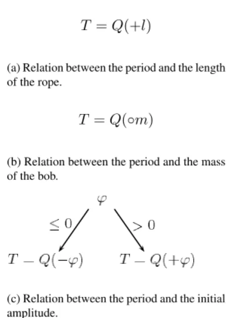
T =Q(+l)
(a) Relation between the period and the length of the rope.
T =Q(◦m)
(b) Relation between the period and the mass of the bob.
(c) Relation between the period and the initial amplitude.
Figure 1: Qualitative models describing the relations be-tween the periodTand the experimentally controlled vari-ables.
for each example. This translates modelling the function’s behaviour into the training of classifiers which predict the qualitative derivative in different parts of attribute space. For instance, the above rules can be acquired by running the CN2 rule learning algorithm on examples labelled by qualitative partial derivatives.
Separate models can be built for each attribute with re-spect to which we observe the function’s behaviour. Alter-natively, one can also build a classifier which predicts all qualitative derivatives at once.
1.2
Introductory example
Consider a set of experiments with a simple pendulum. The task is to learn qualitative relations between the period of the pendulum’s first swing (T), the length of the rope,l, the mass of the bob,m, and the initial angle of displacement,
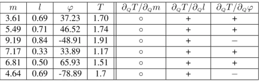
φ. A sample of data collected in such an experiment is shown in Table 1 (first four columns).1
We can then use Padé to compute the qualitative relations for each measurement: ∂QT /∂Qm, ∂QT /∂Ql,∂QT /∂Qφ,
and append them to the original data (Table 1, last three columns). Finally, an algorithm for induction of classifica-tion trees is used to construct a qualitative tree for each qualitative relation, where examples are represented by original attributes and the partial derivative (e.g. one of the last three columns from Table 1) plays the role of the class. The resulting trees are shown in Fig. 1. Two of them have only a single leaf: the period always increases with the length of the rope (T =Q(+l)) and does not depend on the mass of the bob (T =Q(◦m)). The tree describing the relation betweenT andφsays that for negative angles,
T decreases with increasing angle while for positive
m l φ T ∂QT /∂Qm ∂QT /∂Ql ∂QT /∂Qφ
3.61 0.69 37.23 1.70 ◦ + +
5.49 0.71 46.52 1.74 ◦ + +
9.19 0.84 -48.91 1.91 ◦ + −
7.17 0.33 33.89 1.17 ◦ + +
6.81 0.50 65.93 1.51 ◦ + +
4.64 0.69 -78.89 1.7 ◦ + −
Table 1: A sample of data collected by experimenting with a simple pendulum.
gles,Tincreases whenφincreases. We can reinterpret this asT =Q(+|φ|).
1.3
Related work
Mathematical foundations of qualitative reasoning were es-tablished by the work of Kalagnanam and Simon [6, 7, 5], but building on the much older work of Samuelson [9] in economics, as well as the work on qualitative stability in ecology [4, 8].
Many algorithms have, in one way or another, tackled the problem of qualitative model induction from observation data. Algorithms QUIN and epQUIN [11, 10, 2] learn qual-itative trees similar to those in Figure 1, except for a some-what different definition of the relation in the leaf. Qual-itative relations in QUIN are not based on partial deriva-tives, as in Padé, but on qualitative constraints. A constraint
z=M+−(x, y)would state that for every pair of examples
in whichxincreases andy decreases (or stays the same), the function value zincreases. This also implies that the function value depends on no other attributes thanxandy. QUIN constructs such trees by computing the qualitative change vectors between all pairs of examples in the data and then recursively splitting the space into regions which share common qualitative properties, such as the one given above. Although Padé combined with a tree learning algo-rithm can produce a similar tree as QUIN, the two methods are fundamentally different. Besides Padé being merely a preprocessor which can be used with any other machine learning algorithm or visualization technique, the crucial difference is that Padé considers individual examples while QUIN operates on pairs. As one of the consequences, Padé can compute qualitative (or numerical) derivatives for a particular point in the attribute space, while QUIN observes properties of regions of space.
Gerçeker and Say [3] fit polynomials to numerical data and use them to induce qualitative models. LYQUID is designed for modelling dynamic systems, where the data consists of traces sampled in time. We believe that this system could be adapted to also work in static systems.
Padé differs from past methods in being, to our knowl-edge, the only algorithm for computing (partial) derivatives on point cloud data. An important difference between these algorithms and Padé is also that Padé is essentially a pre-processor while other algorithms induce a model. Padé merely augments the learning examples with additional
la-bels, which can later be used by appropriate algorithms for induction of classification or regression models, or for visualization. This results in a number of Padé’s advan-tages. For instance, to our knowledge, most other algo-rithms for learning qualitative models only handle numeri-cal attributes, except for QDE learners which already take qualitative behaviours as input. One variant of Padé can use discrete attributes while computing the derivative, while with others we can use them later, when machine learning algorithms are applied to Padé’s output.
The major contribution of this work, besides the idea of transforming the problem of qualitative modelling to stan-dard induction of classifiers, are methods for computing partial derivatives of an unknown sampled function. In this respect it is related to numerical analysis for estima-tion of partial derivatives. Numerical analysis methods for computing partial derivatives are only useful for a function which isknownin the sense that we can compute its value at any values of arguments which the algorithm requires. These methods are not appropriate for learning from data, where the function is sampled only in a limited number of points.
2
Algorithms
Let f be a continuous function of n arguments, y =
f(x1, x2, . . . , xn). The function is sampled inN points;
the point’s coordinates together with a function value rep-resent a learning example. In machine learning termi-nology, each example is described by a list ofattributes,
(a1, a2, . . . an) and the outcomef(a1, a2, . . . , an). The
basic task of Padé is to compute a partial derivative at each point (learning example)Pin directionxi.
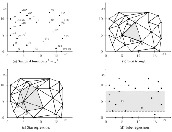
Fig. 2a shows an example of such data for a function
f(x, y) = x2−y2. Each point represents a learning
ex-ample, and the numbers beside the examples give the func-tion values. We will compute the derivative w.r.t. x1 at
P = (5,5)marked by a hollow symbol. Other points used in computation will be marked asA,B,Cand so on. We will treat these points as elements of affine space, and use tA =A−P,tB=B−P,. . . to denote the vectors from
Pto the corresponding points. We will also extend the def-inition off to these vectors, i.ef(tA) = f(A−P) :=
(a) Sampled functionx2−y2. (b) First triangle.
(c) Star regression. (d) Tube regression.
Figure 2: An artificial, sampled function (a) and an illustration of Padé’s methods (b-d).
in which the pointP lies in the centre, tP = 0 and the
corresponding function valuef(tP)equals 0.
Formally, the partial derivative with respect toxiat point
P is defined as
∂f ∂xi
(P) = lim h→0
f(P+hxi)−f(P)
h , (2)
wherexiis thei-th base vector.
This definition cannot be used directly on data since it involves infinitesimally smallhand, furthermore, since we cannot compute the function value at arbitrary points. Ac-cording to Taylor’s theorem, the function can be treated as approximately linear in small neighbourhoods ofP,
f(x1, . . . xn) =b0+ n
∑
i=1
bixi+ϵ, (3)
whereϵrepresents the remainder in Taylor expansion (the function’s non-linearity within the neighbourhood) and also any noise in the data.
The derivative with respect toxi equals bi in (3). The
task is then to define a suitable neighbourhood and esti-mate the coefficientbiaccordingly. We will present three
different ways for solving this problem. The first method determines the linear functionf by simple linear interpo-lation over the simplex while the other two methods use linear regression.
2.1
First Triangle method
First triangle method models the function’s behaviour by dividing the attribute space into simplices (our two-dimensional illustrations show them as triangles) by using the standard Delaunay triangulation [1] as shown in Fig. 2b. Let us assume that there is no noise in the data and that the sample is sufficiently dense so the function is approxi-mately linear within each triangle.
Since the number of unknown coefficients bi in (3)
equals the number of vertices of the simplex, the coeffi-cients can be found analytically by settingϵ= 0. Perform-ing the calculation in vector space instead of in the affine space of points also eliminates the free termb0 and point
P.
Lett1,. . . ,tnbe the vectors fromPto the vertices of the
simplex which lies in directionxi. We look forb1,. . . ,bn
which satisfy
[b1. . . bn][t1. . .tn] = [f(t1). . . f(tn)] (4)
(note thattiaren-dimensional vectors) and thus
[b1. . . bn] = [f(t1). . . f(tn)][t1. . .tn]−1 (5)
For our two-dimensional example (Fig. 2b), we interpo-late over the triangle P AB and compute the coefficients as
[b1, b2] = [f(tA), f(tB)][tA,tB]−1,
which equals
2.2
Star Regression
Star Regression is based on similar assumptions as the First triangle method, but improves its noise resistance by as-suming the function’s linearity across the entire star (the set of simplices surrounding a point) around the pointP
instead of just across a single simplex.
We can no longer use interpolation as in the First trian-gle, as it would result in a system with more equations than unknowns and would usually have no solution. We there-fore allow non-zero error termsϵand translate the problem into computation of univariate linear regression over the vertices in the star.
Ift1,. . . ,tnare the vectors fromP to the vertices of the
star, we computebi, which equals the derivative, as
bi =
∑
jtjif(tj) ∑
jt 2 ji
, (6)
wheretjirepresents thei-th component of the vector
cor-responding to thej-th point in the star,tj.
In our illustration (Fig. 2c), we compute the univariate linear regression over examples A, B, C, D, E and F, and use the first coefficient as derivative.
2.3
Tube Regression
Tube Regression adds even more noise resilience. Instead of triangulating, it considers a certain number of examples in a (hyper)tube passing through pointPin direction paral-lel to the axis of differentiation (Fig. 2d; the tube is repre-sented by the shaded area). We now assume that the func-tion is approximately linear within short parts of the tube and again estimate the derivative from the corresponding coefficient computed by the univariate regression, this time over the examples in the tube.
Since the tube can also contain examples that lie quite far away fromP, we weight the examples by their distances fromP along the tube (that is, ignoring all dimensions but
xi). The weight of thej-th example in the tube equals
wj=e−t 2
ji/σ2, (7)
wheretjiis thei-th component of vectortj(that is, the
dis-tance betweenP and thej-th example in direction parallel to the axis of differentiation, xi). Parameter σis chosen
so that the farthest example in the tube has a user-set neg-ligible weight. As a rule of thumb, we use tubes with 30 examples, with the farthest (e.g.the right-most point in the tube in Fig. 2d) having a weight ofw30= 0.001.
We then use the standard weighted univariate linear re-gression to compute the coefficient of the linear termbi,
bi=
∑
jwjtjif(tj) ∑
jwjt2ji
. (8)
The Tube regression is computed from a larger set of ex-amples, so we can use thet-test to estimate the significance of the derivative. Significance together with the sign ofbi
can be used to define qualitative derivatives in the following way: if the significance is above the user-specified thresh-old (e.g.p≤0.7), the qualitative derivative equals the sign of bi; if significance is below the threshold we define the
qualitative derivative to besteady, disregarding the sign of
bi.
2.4
Time complexity
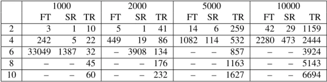
Let N be the number of examples andnthe number at-tributes (function arguments, dimensions).
First triangleandStar regressionmethods are based on Delaunay triangulation. The time complexity of its compu-tation is difficult to assess without making any strong as-sumptions about the data. The state of the art qhull library needs, roughly, O(2nNlogN)to compute the
triangula-tion (a detailed analysis can be found in [1]).
For each data point, the First triangle algorithm needs to find the triangle lying in the desired direction, which re-quires computing the determinant of a n-dimensional ma-trix for every triangle in the star. The time complexity is
O(N n3t), wheretis the maximal number of triangles in any star. The value oft is again difficult to estimate, but it usually rises exponentially with the number of dimen-sions, which makes the time complexityO(N n32n). The
total time complexity, including the triangulation, is thus
O(N2n(logN+n3))
Star regression computes univariate regression at every data point and has a time complexity of O(N s), wheres
is the number of points in the star. Assgenerally rises ex-ponentially with the number of dimensions, the theoretical time complexity of this part of Star regression isO(N2n).
The total complexity is dominated by that of triangulation and thus equalsO(2nNlogN).
Tube regressionfinds the nearest neighbours of each of
N examples, which takesO(nN2), followed by linear re-gression over thek examples in the tube. The total time complexity isO(nN2+k)≈O(nN2).
Since these theoretical time complexities do not offer much insight into the algorithms’ actual running times, we conducted a set of experiments with different num-ber of examples and attributes. The goal function was random since it does not affect the time complexity. All experiments were run on a 2 GHz laptop with 2 GB of RAM. Results (Table 2) indicate that the time complex-ity of triangulation-based methods is indeed exponential in number of attributes and log linear in number of examples, while the Tube regression is linear in number of attributes and quadratic in number of examples. The exponential time complexity prevents the use of triangulation-based methods with more than four attributes.
3
Experiments
1000 2000 5000 10000
FT SR TR FT SR TR FT SR TR FT SR TR
2 3 1 10 5 1 41 14 6 259 42 29 1159
4 242 5 22 449 19 86 1082 114 532 2280 473 2444
6 33049 1387 32 – 3908 134 – – 857 – – 3924
8 – – 45 – – 176 – – 1163 – – 5143
10 – – 60 – – 232 – – 1627 – – 6694
Table 2: Running times (in seconds) of First triangle (FT), Star regression (SR) and Tube regression (TR) methods for calculation of derivatives w.r.t. each attribute on data sets with 1000, 2000, 5000 and 10000 examples and 2, 4, 6, 8, 10 attributes. Symbol – denotes that the program ran out of memory.
discrete attributes. The accuracy is measured by comparing the predicted qualitative behaviour with the analytically de-rived true relation.
3.1
Accuracy
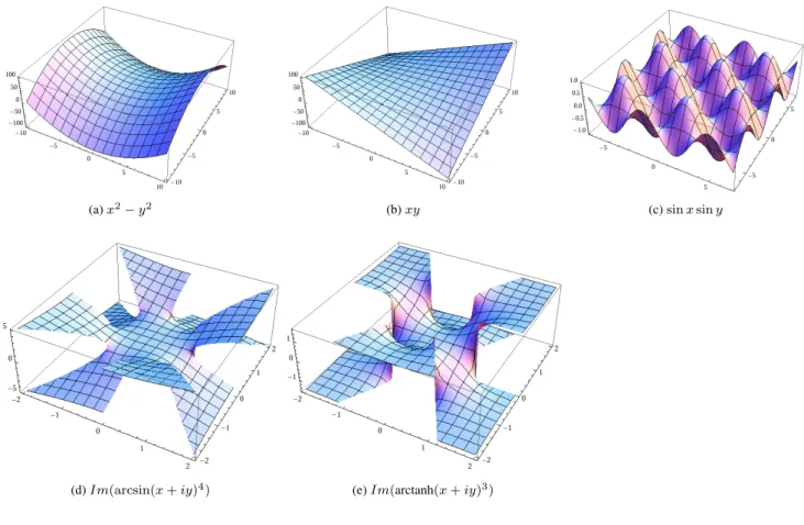
We observed the accuracy of Padé on a few mathematical functions. We estimated partial derivatives using Padé and compared them with the analytically obtained correct an-swers, except for the functions in Fig. 3d and Fig. 3e for which we computed numerical approximations of partial derivatives by Mathematica [14]. Note that this procedure does not require cross-validation or a similar form of data sampling since the known ground truth (the correct deriva-tives) is not used in the induction process.
Functionsf(x, y) =x2−y2andf(x, y) =xy, withx
andy sampled from[−10,10]were used as simple exam-ples of functions which are continuous and differentiable in the whole interval. The heavily oscillating f(x, y) = sinxsiny, withx andy from[−7,7] represents a func-tion whose qualitative behaviour changes frequently, so the partial derivatives are more difficult to compute and model. FunctionsIm(arcsin(x+iy)4)andIm(arctanh(x+iy)3)
in[−2,2]×[−2,2]are two examples of discontinuous func-tions. All functions are visualized in Fig. 3.
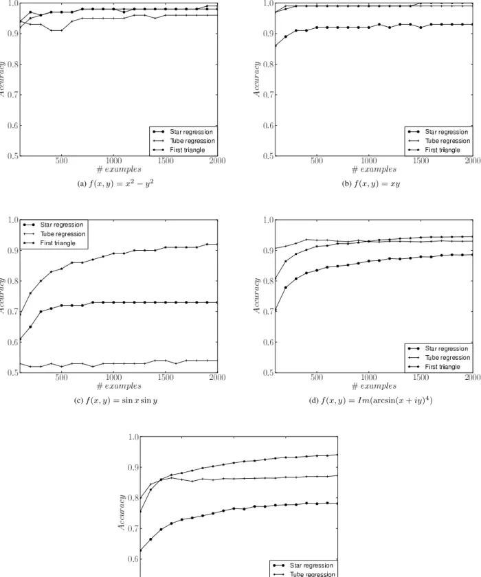
We computed the derivatives and trained the classifiers on ten random samples of 1000 points. Average pro-portions of correctly calculated qualitative derivatives are shown in Table 3. First triangle and Tube regression per-form equally well, except for the Tube regression’s failure onf(x, y) = sinxsiny. A visual exploration of predicted derivatives using a scatter plot clearly shows that this is due to the tube being too long and thus covering multiple periods of the function. Star regression’s performance lags behind those of the other two algorithms.
To estimate the dependence of classification accuracy on data set size we conducted these same experiments on sam-ples of 100 to 2000 data points. We found out that learning curves tend to flatten out at around 500 examples (Fig. 4). The general order of methods w.r.t their accuracy remains the same for all sample sizes, except for the last two func-tions, which are discontinuous and where the First Triangle method seems to suffer the least at very small samples.
3.2
Scalability to high number of
dimensions
We checked the scalability of Padé to high dimensional spaces with an experiment with functionx2−y2, in which
we added 98 attributes with random values from[−10,10]
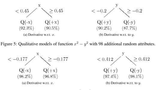
to the data. We use the Tube regression to calculate the derivatives since First triangle and Star regression cannot handle such high dimensional data due to their use of trian-gulation. We analysed the results by inducing classification trees with the computed qualitative derivatives as classes. Trees for derivatives byxandyagree well with the correct results (Fig. 5).
3.3
Robustness to noise
We sampled the functionf(x, y) =x2−y2in 1000 points
withxandyfrom[−10,10], and introduced uniform ran-dom noise of up to±20to the function value. Since the First triangle and Star regression methods suppose no or little noise, we again tested only the Tube regression.
Induced models (Fig. 6) are correct and the split thresh-olds are surprisingly accurate given the huge relative amount of noise at aroundx= 0andy= 0.
3.4
Handling of discrete attributes
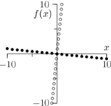
We explored Padé’s handling of discrete attributes on a function defined as
f(x, s) =
{
x/10 ;s= 1 10x ;s= 0
Besides the continuous attributexand boolean attributes, the data set also included an attributerwith random values and no influence on f. Variablesxandrwere from the same definition range, [−10,10]. The function was sam-pled in 400 points.
(a)x2−y2 (b)xy (c)sinxsiny
(d)Im(arcsin(x+iy)4) (e)Im(arctanh(x+iy)3)
Figure 3: Functions used in experiments.
f(x, y) First Triangle Star Regression Tube Regression
∂Qf /∂Qx ∂Qf /∂Qy ∂Qf /∂Qx ∂Qf /∂Qy ∂Qf /∂Qx ∂Qf /∂Qy
x2−y2 98% 98% 98% 97% 95% 95%
xy 99% 99% 92% 92% 99% 99%
sinxsiny 89% 89% 73% 72% 53% 53%
Im(arcsin(x+iy)4) 93% 93% 87% 86% 93% 93%
Im(arctanh(x+iy)3) 91% 93% 76% 79% 86% 90%
Table 3: The comparison of accuracies of Padé’s methods on artificial datasets.
4
Conclusion
We described a new approach to induction of qualitative models whose advantage over (rare) existing similar algo-rithms is that it translates the problem into a standard su-pervised learning problem, which is one of the most re-searched fields in machine learning. The proposed transla-tion requires computatransla-tion of qualitative partial derivatives, which we defined simply as signs of ordinary partial deriva-tives. The biggest problem – and with that the core of this paper – is computation of partial derivatives of the function which is being modelled. Standard methods from numer-ical analysis cannot be applied here since they require a known function whereas in our case the function value is known only in a finite number of sampled examples.
We proposed three methods for this task. Two are based
on triangulation and suppose either no noise or a small amount of noise. Besides this, the two methods are not likely to be useful in real-world scenarios which often con-tain more attributes than triangulation can handle. Exper-iments with the time complexity of the methods clearly show that the triangulation-based methods are unable to handle more than 6 attributes. Nevertheless, in absence of noise these two methods provide very good accuracy for functions with complex qualitative behaviour and low num-ber of arguments, such asf(x, y) = sinxsiny. Tube re-gression on the other hand offers robustness to noise, scales well to high dimensional spaces and can also handle dis-crete function arguments with proper definition of metrics.
(a)f(x, y) =x2−y2 (b)f(x, y) =xy
(c)f(x, y) = sinxsiny (d)f(x, y) =Im(arcsin(x+iy)4)
(e)Im(arctanh(x+iy)3)
(a) Derivative w.r.t.x. (b) Derivative w.r.t. toy.
Figure 5: Qualitative models of functionx2−y2with 98 additional random attributes.
(a) Derivative w.r.t.x. (b) Derivative w.r.t. toy.
Figure 6: Qualitative models of functionx2−y2with added random uniform noise.
learning method.
We have put the methods at a practical test within Euro-pean project XPERO (IST-29427). Our goal was to provide a robot with an algorithm for autonomous learning. We found qualitative models most suitable for this task. For example, a particular case was to discover the relation be-tween the area of the ball in the image from robot’s camera, and the robot’s angle and distance from the ball [13]. The robot learnt that the area of the ball is increasing with de-creasing distance and dede-creasing with inde-creasing angle (the robot turning away from the ball, so it gradually vanishes from the robot’s field of view).
Since the field of learning qualitative models from data is rather unexplored, the paper opens more new interesting questions than it answers. Pioneers of qualitative modelling who constructed the models manually were able to describe real phenomena using simpler models, not unlike the clas-sification trees and rules presented here. Is this generally the case? Do simple learning algorithms like tree induction, suffice, or will actual problems require more sophisticated algorithm, such as, for instance, support vector machines?
This paper follows the mathematical definition of partial derivative which is essentially univariate. Partial deriva-tives are linear and do not interact: the effect of changing two quantities at the same time equals the sum of effects of changing each of them separately. The exception to this rule are certain kinds of singularities. Does this happen in practice, especially in qualitative descriptions of problems? Can it happen, for instance, that two economic measures used separately decrease the inflation while using both to-gether would increase it? Is treating each attribute sepa-rately indeed appropriate? We leave these questions open for further research.
Acknowledgements
This work was supported by the Slovenian research agency ARRS (J2-2194, P2-0209) and by the European project
XMEDIA under EC grant number IST-FP6-026978.
References
[1] C. Bradford Barber, David P. Dobkin, and Hannu Huhdanpaa. The quickhull algorithm for convex hulls. ACM Transactions on Mathematical Software, 22(4):469–483, 1996.
[2] Ivan Bratko and Dorian Šuc. Learning qualitative models.AI Magazine, 24(4):107–119, 2003.
[3] R. K. Gerçeker and A. Say. Using polynomial approx-imations to discover qualitative models. InProc. of the 20th International Workshop on Qualitative Rea-soning, Hanover, New Hampshire, 2006.
[4] Clark Jeffries. Qualitative stability and digraphs in model ecosystems.Ecology, 55(6):1415–1419, 1974.
[5] Jayant Kalagnanam and Herbert A. Simon. Directions for qualitative reasoning.Computational Intelligence, 8(2):308–315, 1992.
[6] Jayant Kalagnanam, Herbert A. Simon, and Yumi Iwasaki. The mathematical bases for qualitative rea-soning.IEEE Intelligent Systems, 6(2):11–19, 1991.
[7] Jayant Ramarao Kalagnanam.Qualitative analysis of system behaviour. PhD thesis, Pittsburgh, PA, USA, 1992.
[8] Robert M. May. Qualitative stability in model ecosys-tems.Ecology, 54(3):638–641, 1973.
[9] Paul A. Samuelson.Foundations of Economic Analy-sis. Harvard University Press; Enlarged edition, 1983.
(a) Modelled function; filled and hollow circles represent ex-amples withs= 1ands= 0, respectively.
(b) Qualitative tree based on Tube Regression.
Figure 7: The function used in the experiment with discrete attributes and the corresponding qualitative model.
[11] Dorian Šuc and Ivan Bratko. Induction of qualitative trees. In L. De Raedt and P. Flach, editors, Proceed-ings of the 12th European Conference on Machine Learning, pages 442–453. Springer, 2001. Freiburg, Germany.
[12] Dorian Šuc, Daniel Vladušiˇc, and Ivan Bratko. Qual-itatively faithful quantitative prediction. Artificial In-telligence, 158(2):189–214, 2004.
[13] Jure Žabkar, Ivan Bratko, and Janez Demšar. Learn-ing qualitative models through partial derivatives by Padé. InProceedings of the 21th International Work-shop on Qualitative Reasoning, Aberystwyth, U.K., 2007.