ROBUST CLUSTERING METHODS WITH SUBPOPULATION-SPECIFIC DEVIATIONS
Briana Joy Kennedy Stephenson
A dissertation submitted to the faculty of the University of North Carolina at Chapel Hill in partial fulfillment of the requirements for the degree of Doctor of Philosophy in
the Department of Biostatistics in the Gillings School of Global Public Health.
Chapel Hill 2017
Approved by:
Amy Herring David Dunson Andrew Olshan
c ○ 2017
ABSTRACT
Briana Joy Kennedy Stephenson: Robust Clustering Methods with Subpopulation-specific Deviations
(Under the direction of Amy Herring)
Large populations have been found to be composed of a unique set of subpopula-tions. Each subpopulation tends to exhibit similar behaviors and respond to various outcomes different from other subpopulations. Mixture models have become a great utility in modeling these differences, by attributing each subpopulation its own unique distribution. The underlying subpopulation inferred from the mixture model is referred to as a latent class or cluster.
Traditional clustering methods operate under the assumption that two subjects allocated to the same cluster will respond identically to all measured variables. Yet, aberrations between some individual measured variables can yield valuable information. Furthermore, these models often realize an increasing number of clusters that expand with the dimensionality of sample size and number of variables. This may lead to a loss in interpretability, due to a large number of clusters and an oversensitivity to minor deviations that exist among groups.
Second, we build upon this to create a predictive clustering model that links the clustering model generated from the RPC with a response probit model via a supervised RPC joint model. Here, subjects more likely to exhibit the outcome of interest can cluster in accordance with her global and local profiles.
ACKNOWLEDGMENTS
Although we’ve come to the end of the road...unlike Boyz II Men, I can definitely let go. This chapter of my life has been filled with many changes and transitions, but also a lot of growth and maturity. I’m grateful for my village of families that have brought me through. I would be remiss if I did not acknowledge them all.
First and foremost, I want to thank my Lord and Savior, Jesus Christ. If He can bring you to it, He will bring you through it. I am grateful for scriptures likeMatthew 6:25-34, andPhilippians 4:13to lean on as I navigated through this process. Thank you for placing spiritual warriors in my life, like Big Sister Althea to provide me spiritual guidance and mentorship as I weathered my time through the wilderness of grad school at North Carolina.
To my big brother Chris, thank you for setting the pace and instilling a competitive hunger inside of me to try and learn everything you knew and then some, so that I could beat you in Family jeopardy on long road trips. You inspired me to learn how to teach myself which became a vital skill in getting through this dissertation. To my younger brother Jonathan, thank you for your constant memes and reminders that grad school was only temporary, and I should hurry up and get out so I could be a real adult with a job. To my baby brother Gavin, thank you for the love and support, and for respecting your place in the birth order to never tease or pick on me for being what was perceived as the eternal student.
for your words of inspiration, care packages, and labors of love. Special thanks to my late Aunt Jacqueline, who was hesitant about me taking a year off between my masters and PhD. She thought after working for awhile, I wouldn’t want to go back. After her death, I found some old letters she typewrote in a box in her storage room, and I understood why. You have been with me in spirit always. Thank you for the motivation to not only go back, but also to finish.
Thank you to my Delta family. I am grateful for each and every connection that has been made from my line sisters of Maksusi to my collegiate chapter of Xi Tau and my graduate chapter in Chapel Hill. You all have given me a shoulder to lean on, and ear to listen, a meal to eat, a bed to crash, a heart to open, a verse to meditate, and a bond that will never break. Quack. Hi roomie! Thank you to my volleyball family for providing me the opportunity to have an outlet to exercise my academic frustrations out in a healthy manner, as well as helping me amass all the championship t-shirts in my closet for all the IM/co-ed season and tournament championships we won. We had some good seasons, some bad ones, and some ugly ones, but you will always be my teammates for life.
Thank you to all the friends that were with me before I started this journey, and are still with me today; from the Beantown Blacktop, HoCo homies, G-Dub-Buds, and the strong side to left side. Thank you for your patience and cooperation with my demanding, sleepless and highly stressful schedule. Thank you for reminding me to not neglect my personal health and relationships in pursuit of my academic goals. And thank you to Hangouts, WhatsApp, FaceTime, iMessage and GroupMe for keeping me close when I felt so far away.
Thank you for all the mindless, yet captivating conversations about everything and nothing at the same time; the messages that made me smile when school made me want to frown; and for encouraging me to focus on the happy, instead of wallowing in the bad. Your positivity and optimism became infectious and you allowed me to grow comfortable in my vulnerabilities. I’m not sure what this chapter would have looked like without him, but it was a lot easier with him in it.
Thank you to my UNC family. First, my adviser, Dr. Herring, thank you for all of your guidance, support and encouragement. You introduced me to bayesian analysis, which has opened the door to a myriad of interesting projects, opportunities, and travel I never thought I would experience as a graduate student. Over the past six years, I have watched and admired how you have made waves in a male-dominated field with your energetic tenacity and enthusiasm. You are an inspiration to the kind of academic researcher I hope to one day be. You have motivated me to continue to keep pushing through the barriers of academia, and not be deterred with any obstacles that will come my way. You unlocked a box of passion and excitement for this subfield, and I can’t wait to share it with the world. Thank you to Dr. Edwards for his coach-player mentorship style that gave me for the grit to survive and thrive in this program. You were the first Black biostatistics professor I had ever met, and it was assuring to know we do exist.
biostatisticians working in different professional fields, and if the pilot should involve a husband peeing in the oven or a TV remote going through the rinse cycle.
TABLE OF CONTENTS
LIST OF TABLES · · · xiv
LIST OF FIGURES · · · xvi
CHAPTER 1: INTRODUCTION · · · 1
CHAPTER 2: LITERATURE REVIEW · · · 3
2.1 Number of Latent Classes Known . . . 3
2.1.1 Latent Class Analysis . . . 3
2.1.2 Frequentist Estimation . . . 4
2.1.3 Bayesian Estimation . . . 6
2.2 Number of Latent Classes Unknown . . . 7
2.2.1 Dirichlet Process . . . 7
2.2.2 Hierarchical and Nested extensions . . . 9
2.2.3 Overfitted Finite Mixture Model . . . 12
2.2.4 Partial Process . . . 12
CHAPTER 3: ROBUST PROFILE CLUSTERING · · · 16
3.1 Introduction . . . 16
3.1.1 Multivariate Categorical Dietary Data . . . 16
3.1.2 Standard Clustering Methods . . . 17
3.2 Robust Profile Clustering . . . 20
3.3 Posterior Computation and Inference . . . 22
3.4.1 Results . . . 27
3.5 Analysis of National Birth Defects Prevention Study Data . . . 28
3.5.1 Multivariate Categorical Dietary Data . . . 28
3.5.2 MCMC Performance . . . 30
3.5.3 NBDPS Results . . . 30
3.6 Discussion . . . 37
CHAPTER 4: SUPERVISED ROBUST PROFILE CLUSTERING · · · 38
4.1 Motivation . . . 38
4.2 Supervised RPC Joint Model . . . 39
4.2.1 Robust Profile Clustering Predictor Model . . . 39
4.2.2 Probit Regression Response Model . . . 41
4.3 Methods . . . 42
4.3.1 Parameter Estimation . . . 42
4.3.2 MCMC Algorithm . . . 43
4.4 Application to National Birth Defects Preven-tion Study . . . 45
4.4.1 NBDPS Dietary Data . . . 45
4.4.2 Comparative Analysis . . . 47
4.4.3 Demographic Confounding . . . 54
4.5 Extension to Local Deviations . . . 56
4.6 Discussion . . . 58
CHAPTER 5: MACHINE LEARNING APPROACHES · · · 60
5.1 Background . . . 60
5.1.1 Dietary Pattern Analysis . . . 60
5.1.3 Machine Learning . . . 62
5.2 Introduction of Machine Learning Methods . . . 62
5.2.1 Robust Profile Clustering . . . 62
5.2.2 CrossCategorization for Approximate In-ference in Nonparametric Bayes Models . . . 64
5.2.3 General concept . . . 64
5.3 Analysis of NBDPS Dietary Data . . . 67
5.3.1 NBDPS Data . . . 67
5.3.2 RPC Results . . . 69
5.3.3 CrossCat Results . . . 72
5.3.4 Comparison of Methods . . . 80
5.4 Discussion . . . 81
CHAPTER 6: CONCLUSION · · · 85
APPENDIX A: MATLAB CODE FOR CHAPTER 3 · · · 86
APPENDIX B: MATLAB CODE FOR CHAPTER 4 · · · 99
APPENDIX C: ADDITIONAL TABLES FOR CHAPTER 5 · · · 114
LIST OF TABLES
3.1 Simulation results of models. A small cluster is defined as any cluster containing less than 5% of
the population size . . . 27
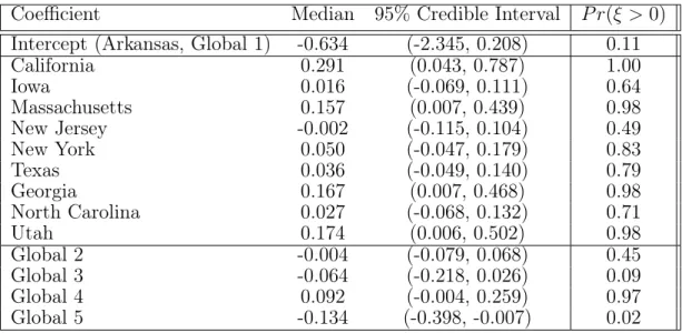
4.1 Parameter estimates of supervised RPC joint
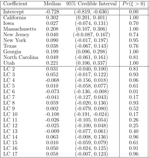
model covariates . . . 50 4.2 Coefficient parameter estimates of LCA Model
0, where LC denotes latent class and the refer-ent group (Arkansas, Global 1) is parameterized
through the intercept . . . 52 4.3 Top 5 foods for each LCA cluster that are most
likely to be consumed at a high consumption level . . . 53 4.4 Descriptive statistics of NBDPS participants
in-cluded in study . . . 55 4.5 Probit Regression model fixed effect parameter
estimates for any oral cleft outcome, Arkansas and Global profile 1 are parameterized in the
intercept term as the referent group . . . 56
5.1 Foods clustered for each view. Names corre-spond to commonalities shared amongst food in
each view . . . 76 5.2 Frequency Distribution of each observed cluster
within each view containing at least 5% of the
population, n (%). . . 77 5.3 True versus predicted percentile consumption of
4 randomly selected foods and 4 randomly se-lected subjects, under different algorithmic
con-ditions. . . 79
C1 Mean Percentile consumption of Foods
Observation-Cluster for Western Alternative and Squash view . . . 114 C2 Mean Percentile consumption of Foods and
C3 Mean Percentile consumption of Foods and
Observation-Cluster for M-Minerals View . . . 116 C4 Mean Percentile consumption of Foods and
LIST OF FIGURES
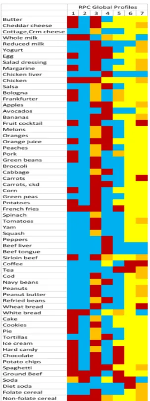
3.1 Heat map showing modal consumption level of RPC global profiles. Blue - no consumption, yel-low - yel-low consumption, orange - medium
con-sumption, red - high consumption. . . 32 3.2 Top 5 foods most likely to be consumed at each
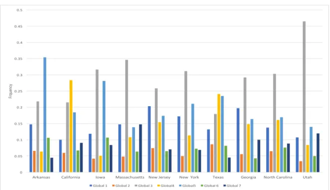
level of global profiles . . . 33 3.3 Frequency distribution of global profiles by
sub-population (state) for the global profiles
identi-fied in the model . . . 34 3.4 Heat map illustrating foods with a tendency to
deviate from the global profile (νj(s) < 0.5), by subpopulation. Blue - no consumption, yellow - low consumption, orange - medium
consump-tion, red - high consumption. . . 36 4.1 Heatmap showing modal cluster patterns of RPC
global profiles. Legend: Blue-no consumption, Yellow-low consumption, Orange-medium
con-sumption, Red-high consumption . . . 48 4.2 Top 5 foods most likely to be consumed at each
level of global profiles derived from RPC
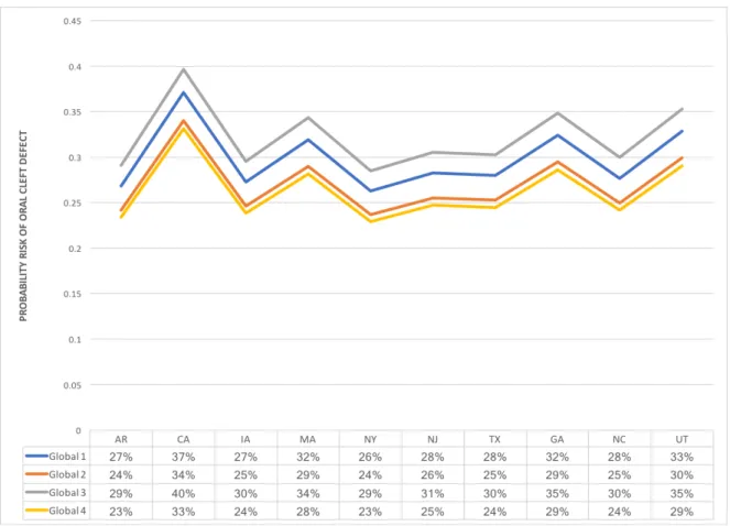
predic-tor model . . . 49 4.3 Plot of unadjusted prevalence rate of orofacial
cleft by state . . . 51 5.1 RPC global profile patterns. . . 69 5.2 Top 5 foods most likely to be consumed at each
level of global profiles . . . 71 5.3 Heat map illustrating foods with a tendency to
deviate from the global profile (νj(s) < 0.5), by subpopulation. Blue - no consumption, yellow - low consumption, orange - medium
5.4 Heatmap showing the clustering patterns of the
63 foods. Each color represents a unique cluster . . . 74 5.5 Heatmap showing the clustering pattern of the
9010 observations. Each color represents a unique
cluster. . . 78 5.6 Heatmap showing which subjects remained
to-gether from LCA model to RPC model (left). Heatmap showing concordance of derived pat-terns from RPC global profiles and traditional
LCA model (right). . . 81 5.7 Concordance heatmaps illustrating which
sub-jects remained together between the LCA and
CrossCat . . . 83 5.8 Concordance heatmaps illustrating which
sub-jects remained together between the RPC and
CHAPTER 1: INTRODUCTION
Model-based clustering methods have been widely used to illustrate differences that exist among subjects in a population. They are especially useful for data reduction when the number of responses collected per subject is large and needs to be condensed for effective inference. The complexities of the data dictate the appropriate method to apply.
The general framework of the mixture model works under the assumption that a given population is composed of a set of groups or components, which we will refer to as clusters. Given a set of outcome variables, subjects are assumed to respond simi-larly with other subjects within the same cluster group, and differently from subjects who belong to a different cluster group. The mixture model construct is composed of two parts illustrated in equation 1.1; a mixing component weight that describes the proportion of the population that belongs to a given cluster, P(zik), and the cluster specific density function that models how the subjects are expected to behave within each cluster group, f(yij|zik). The basic setup is illustrated as,
f(yi) = K X
k=1
P(zik) p Y
j=1
f(yij|zik) (1.1)
where p is the number of response items and K is the number of identifiable
clus-ters in the population. The observed response of subject i ∈ (1, . . . , n) for variable
fit to an appropriate continuous probability distribution. Discrete level data is fit to an appropriate discrete probability distribution.
CHAPTER 2: LITERATURE REVIEW
2.1 Number of Latent Classes Known
2.1.1 Latent Class Analysis
The most common clustering method for multivariate categorical response data is the latent class model. First introduced by Lazarsfeld and Henry (1968), the latent class model is a finite mixture model where the response data is fit according to a multinomial distribution. The number of clusters is prefixed and stationary. It assumes the population will aggregate into exactlyK clusters.
Let y1, ...,yn be the set of n subjects observed, and yi = yi1, ..., yip represent the observed response data for subject ifor a set of p variables. Further, let each response
variable have d categorical levels such that yij = c and c ∈ (1, . . . , d). The cluster assignment of subject i is denoted zi = (zi1, . . . , zik), where zi is a K-length binary vector that is mutually exclusive and exhaustive. If subjectiis assigned to classk, then zik = 1andzik0 = 0, whenk0 6=k. LetP(zik = 1) =πkfor all subjectsi∈(1, . . . , n)and PK
k=1πk= 1. Given multivariate categorical responses, we letP(yij =c|zik = 1) =θjc|k and θj·|k denote the d−length probability vector for response j within cluster k, such that Pd
c=1θjc|k = 1. Therefore, the likelihood function can be illustrated as,
f(yi|zi) = K X
k=1
πk p Y
j=1 d Y
c=1
θ1(yij=c|zik=1)
jc|k (2.1)
The parameters πk, θj·|k can be estimated from either a frequentist or a Bayesian perspective. The frequentist perspective relies on maximum likelihood estimation of the parameters given the complete likelihood function.
L(y) = n X
i=1
f(yi) = n X i=1 K X k=1 πk p Y j=1 d Y c=1
θ1(yij=c|zi=k)
jc|k . (2.2)
2.1.2 Frequentist Estimation
Formalized by Dempster et al. (1977), the EM algorithm treats zik as the “miss-ing” variable for individual i. The expected unobserved cell counts are computed in
the E-step using the observed data and provisional parameter estimates. Those ex-pected values are then maximized in the complete data log-likelihood function to make updated provisional parameter estimates for the next iteration. This continues until some form of convergence is reached with the difference between the current and pre-vious iteration very small. To obtain parameters that maximize the log-likelihood, a Lagrange multiplier is included in the log-likelihood equation to impose the restriction that PK
k=1πk= 1.
L(y) = N X i=1 K X k=1 ˆ
δik·log πk p Y j=1 d Y c=1
θ1(yij=c|zik=1)
jc|k −λ(
K X
k=1
πk−1) !
(2.3)
EM-algorithm
1. E-step: calculate posterior probability of class membership weight for individ-ual i using estimates of previous iteration: δˆik = P r(zik = 1|Yi = yi) =
πkQpj=1
Qd c=1θ
1(yij=c|zik=1)
jc|k
PK
m=1πmQpj=1Qdc=1θ
1(yij=c|zim=1)
jc|m
2. M-step: Maximize the expected log-likelihood withPK
the following updated parameters:
˜
πk = PN
i=1δˆik
N ,
˜
θjr|k = PN
i=1δˆikI(yij =r) PN
i=1δˆik
3. Continue iterations untilkδ˜ik−δˆikk< , whereδ˜ik andδˆik denote the current and previous iterated values, respectively, and is a preset threshold value.
The EM algorithm does not require much information on the initial parameter val-ues, but the computation can be burdensome and convergence slow. Newton-Raphson (NR) offers a more rapid convergence, but only when the initial parameter estimates are close to the final solution. In the NR method, log-likelihood scores and double derivatives of the parameters are used iteratively and are able to provide parameter standard errors. Score functions are calculated for all free parameters:
∂L(y)
∂πk = N X i=1 Qp j=1 Qd c=1θ
1(yij=c|zik=1)
jc|k PK
m=1πm Qp
j=1 Qd
r=1θ
1(yij=c|zim=1)
jc|m
for all K −1 class variables, since PKk=1πk= 1.
∂L(y)
∂θjc|k = N X i=1 δik
1(yij =c|zik = 1)
θjc|k
− 1(yij =d|zik = 1)
1−Pd−1c=1θjc|k !
for all j = 1, ..., p item responses, k = 1, ..., K classes, and c = 1, ...d−1 categorical indicators, since Pd
2.1.3 Bayesian Estimation
Bayesian methods provide efficient and stable estimates in the case of a latent class model. For example, in the case of the NR method, the Hessian matrix contains the double derivative of parameters and often encounter inversion issues and ultimately poor standard error estimates, which can be overcome with Bayesian techniques. Pos-terior computations are rather straightforward for the traditional LCA. Both πk and
θj·|k are multinomially distributed and can be estimated using conjugate Dirichlet pri-ors. Simple execution of the Bayesian estimation is available in a convenient R package, BayesLCA(White et al. 2014).
Gibbs sampler
1. Set starting values by sampling from prior:
π1, . . . πK ∼Dir(α1, . . . , αK)
θj·|k∼Dir(η1, . . . , ηd),
for all responsesj ∈(1, . . . , p)and clusters k∈(1, . . . , K). If prior information is known about the respective hyperparameters, they can differ from one another. Most times, prior information is unknown and a symmetric Dirichlet distribution is assumed such that α1 =. . .=αK for the mixing component hyperparameters and η1 =. . .=ηd for all density parameters.
2. Calculate posterior probability of membership to cluster k ∈ (1, . . . , K) for all
i= 1, ..., n subjects.
δik =P r(zik = 1|Yi =yi) =
πkQpj=1Qdc=1θ
1(yij=c|zik=1)
jc|k PK
m=1πm Qp
j=1 Qd
c=1θ
1(yij=c|zim=1)
3. Assign cluster membership for all i= 1, ..., nsubjects, zik ∼M ult(δi1, ..., δiK).
4. Update mixture component weights: π1, . . . , πK ∼ Dir(α1 +n1, ..., αK +nK), wherenk denotes the number of subjects currently allocated to cluster k.
5. Update cluster-specific density parameters for all j ∈(1, ..., p) response variables and k ∈ (1, ..., K) latent classes: θj1|k, . . . , θjd|k ∼ Dir(η1+nj1|k, . . . , ηd+njd|k), wherenjc|k denotes the number of subjects in clusterk that observed aclevel of response j.
In both frequentist and Bayesian estimation techniques, if the correct number of classes is unknown, several models may be fit with varying K-values. Posthoc analysis
is required in order to determine the best model fit such as AIC, BIC, DIC, Bayes Factor, and the Lo-Mendell-Rubin tests (Nylund et al. 2007).
2.2 Number of Latent Classes Unknown
2.2.1 Dirichlet Process
When the number of clusters is unknown, the need for multiple models and posthoc analysis can be avoided with the implementation of a prior on the number of latent classes. In the mixture model case, finite mixture component weights are replaced with an infinite set of mixture component weights. These are then generated from a stick-breaking distribution known as theGriffiths-Engen-McCloskey (GEM) process, where
π|α ∼GEM(α),
νk ∼ B(1, α)
πk =νk Y
l<k
(1−νl).
Extending to the remaining model parameters we develop the Dirichlet process mixture model, where againθk denotes the set of parameters attributed to cluster k,
θk∼P0
G=
∞ X
k=1
πkδθk
G∼DP(α, P0),
(2.5)
The implementation of the Dirichlet process on a mixture model of multivariate categorical data was demonstrated by Dunson and Xing (2009), and works under the following subject-specific distribution,
f(yi|θk, z) = ∞ X k=1 πk p Y j=1 d Y c=1
θI(yij=c|zik=1)
jc|k (2.6)
This removes the restriction on the number of clusters possible in the model. Given the discrete nature of our model, P0 is defined to have a base Dirichlet distribution. The number of nonempty clusters grows at a rate of α log n (Antoniak 1974), where α denotes the scale precision or concentration parameter of the Dirichlet process. The
concentration parameter takes on a role of confidence in the model’s ability to identify the correct number of clusters. For a convenient Gibbs sampling of posteriors, the same stick-breaking construction described in Equation 2.4 is used.
Prior set-up
α∼Γ(aα, bα)
θj·|h ∼Dir(φ, . . . , φ)
νk ∼Beta(1, α), πk =νk k−1 Y
h=1
Posterior Computation
1. Update zi ∼M ult(δi1, . . . , δik).
δik =
πk Qp
j=1 Qdj
c=1θ
1(yij=c|zik=1)
jc|k PK
h=1πh Qp
j=1 Qdj
c=1θ
1(yij=c|zih=1)
jc|h
2. Updateθjc|kfor all exposure levels,c∈1, . . . , dj of individual variablej ∈1, . . . , p in latent clusterk ∈1, . . . , K.
θjc|k ∼Dir(φ+nj1|k, . . . , φ+njdj|k)
3. Update π ={πk}∞k=1.
νk ∼Beta(1 +nk, α+ K X
l=k+1
nk),
πk =νk k−1 Y
h=1
(1−πh)
4. Update α∼Γ(aα+K, bα−Pkh=1log(1−πh))
2.2.2 Hierarchical and Nested extensions
identify the subpopulation index in the model.
G0|γ, H ∼DP(γ, H)
Gs|α, G0 ∼DP(α, G0)
θsk|Gs ∼Gs
Gs = ∞ X
k=1
πskδθ∗
k
(2.7)
In this case, each subpopulation distribution is drawn from the same Dirichlet process
DP(α, G0), where G0 is a measure drawn from a common overall DP characterized by strength parameter γ and base measure H. Therefore, the HDP model contains
multiple subpopulation specific distributions that may or may not contain similarities with other distributions in different subpopulations.
Nested approaches cluster subjects across distributions nonparametrically (Rodriguez et al. 2008, Hu et al. 2017). Nested Dirichlet process (NDP) is convenient for allowing adaptive clustering to occur at more than one level. Groups can be unique and exhibit varying behaviors from other groups. Consider a set of subpopulation distributions
F1, . . . , FS, where S denotes the number of subpopulations that comprise the overall population.
yi·|θsl ∼Fθsl
θ∗sl|Gj ∼Gj
Gj ∼ ∞ X
s=1
πsδG∗
s
G∗s ∼
∞ X
l=1
ωslδθ∗sl
(2.8)
with θsl ∼ H, where H is a probability measure on the Borel sets of Θ. Dirac delta functionsδθ∗sl, δG∗
s denote probability measures concentrated atθ
∗
G∗s, respectively. Mixing weights,ωslandπsare both drawn independently from a GEM distribution.
ωsl =νsl∗ L−1 Y
k=1
(1−νsk∗ ), whereνsl∗ ∼Beta(1, β)
πh∗ =υh∗
S−1 Y
k=1
(1−υk∗), where υh∗ ∼Beta(1, α)
To facilitate in estimation and posterior computations, an LS-truncation is imple-mented. S is maximized at the total number of subpopulations included in the dataset,
and L is maximized at an overestimation of the number of latent classes.
Approaching from the mixture model perspective, let l represent the cluster
in-dex such that l = 1, . . . , Ls, and Ls denotes the maximum number of clusters within subpopulation s. Let y(si)
ij denote observed response level of variable j from subject
i= 1, . . . , nthat belongs to subpopulation sand zil(s), the binary indicator determining
if subject i belongs to cluster l within subpopulation s. Let θsl· denote the support parameters of the cluster distribution of latent cluster l of subpopulation s.
f(yi|zsi) = S X s=1 πs Ls X l=1 ωsl p Y j=1
f(yij|z (s) il ),
where ωsl denote the mixing weight probability that a subject from subpopulation
s belongs to latent class l. Let πs denote the mixing weight probability that latent cluster l belongs to subpopulation s. Intuitively, it is clear that the number of latent
classes within each subpopulation are embedded inside another DP that denotes the number of groups or subpopulations.
Limitations
actually exist (Miller and Harrison 2013). The number of identifiable clusters increase as the sample size increase. An imposition of sparsity is necessary to allow for an interpretable number of clusters to make efficient inference in settings we will consider. Additionally, with a large number of variables(p), it is possible that subjects allocated to the same cluster may behave differently for a few exposures.
2.2.3 Overfitted Finite Mixture Model
An alternative to the Dirichlet Process mixture model is the overfitted finite mixture model. Asymptotically, a finite model with an exceedingly largeK will behave similar
to the DP mixture model, and consistently identify the number of nonempty clusters of a given population (Rousseau and Mengersen 2011). The model is setup as it was in Equation 2.1, where K is now set to an exceedingly high number, K ≡ Kmax >>
KT RU E, with the expectation that after MCMC, the correct number of clusters will
remain nonempty.
The accuracy of this model remains highly sensitive to the selection of the Dirichlet hyperparameter on πk. The Dirichlet hyperparameter is preset to 1/Kmax, which
en-courages a certain level of sparsity by asymptotically shrinking the number of nonempty clusters in the model towards the truth (Gelman et al. 2014). This slight dependency ofKmax on the Dirichlet hyperparameter value can affect the tendency of extra clusters from expectedly shrinking to zero. Accurate prior value determination can be rectified with parallel prior tempering, but this can be a heavy computational burden with high dimensional datasets (van Havre et al. 2015).
2.2.4 Partial Process
variables included in the set. Alternatively, methods have been created that allow subjects to cluster at a global and local level. In the hybrid Dirichlet mixture model, subjects are clustered locally by each individual variable, and then globally based on combinatorial similarities of local cluster indices (Petrone et al. 2009). This approach is achieved by allowing a local partitioning scheme for every individual variable, coupled with a joint distribution to cluster all of the individual variables globally. Consider a set ofptotal variables,(θ1, . . . , θp), wherekj denotes the cluster profile index of variable
j. Let G denote a distribution function on Rp, and a prior on
G=
K X
k1=1
· · ·
K X
kp=1
py1,...,yp(k1, . . . , kp)δ1k1,...,pkp (2.9)
Each local clustering profile is marginally distributed with a random distribution func-tion, that can be finite (e.g. Dirichlet distribution) or infinite (e.g. Dirichlet Process). The individual variable cluster indices are jointly processed together via p(k1, . . . , kp), which denotes the global weight of subjects that share the same vector of label combi-nations. This joint labelling function is drawn from a hidden labeling process, using a copula construction.
While useful in functional data analysis, this method faces challenges in the ap-plication to multivariate categorical data. MCMC computation becomes increasingly burdensome with an increasing number of variables, aspincreases (Petrone et al. 2009).
Additionally, the copula construction used to derive the global clustering scheme is not unique when handling discrete data, which poses a problem in distinguishing behaviors amongst the different global cluster assignments (Smith and Khaled 2012).
population, while maintaining a global cluster assignment for all other variables. This process allows subjects to cluster with other subjects that behave similarly for most or some of the variables analyzed. It also reduces noise that may arise from variables that do not provide much information to an overall population pattern.
Let Gij denote the binary indicator on whether exposure outcome j ∈(1, . . . , p) of subject i∈(1, . . . , n) belongs to a global cluster,(Gij = 1), or local cluster, (Gij = 0), determined by allocation probability parameter νj. Let φij denote the local cluster membership index for exposure outcome j ∈ (1, . . . , p) and φi0, the global cluster
membership index for subject i ∈(1, . . . , n). The subject-specific cluster membership index φi· are drawn from the stick-breaking representation of the Dirichlet process (Sethuraman 1994).
Gij ∼Bern(νj), νj ∼ B(1, β)
φij ∼ ∞ X
h=1
πjhδh,
πjh =π∗jh Y
l<h
(1−πjl∗), πjh∗ ∼ B(1, α)
(2.10)
This formulation allows for a unique clustering scheme of each individual exposure outcome. The hyperparameter α controls how rapidly mixture component weight πjh decreases to0as the number of clusters increase. Hyperparameterβ controls the overall
weight on each of the local exposure components. However, in applications where n
and p are large, a more sparse alternative is availabele that collapses the probability
Gij ∼Bern(νj), νj ∼ B(1, β)
φij ∼ ∞ X
h=1
πhδh,
πh =πh∗ Y
l<h
(1−πl∗), π∗h ∼ B(1, α)
(2.11)
CHAPTER 3: ROBUST PROFILE CLUSTERING
3.1 Introduction
3.1.1 Multivariate Categorical Dietary Data
Food frequency questionnaires (FFQ) are often used to measure an individual’s dietary intake over a period of time. The standard FFQ queries on consumption/intake levels of over 100 foods (Subar et al. 2001). Some researchers focus on individual foods or nutrients, but these foods are not consumed in isolation, and many nutritionists argue that a more holistic approach is needed (Motulsky et al. 1989). When data includes a large number of exposures or in the case of an FFQ, food items, data reduction techniques such as factor analysis, latent class analysis, or other clustering approaches are often used (Kant 2004, Venkaiah et al. 2011, Sotres-Alvarez et al. 2010, Keshteli et al. 2015).
residence, the foods consumed to characterize “American” diets would look different, due to regional differences. A healthy diet may incorporate an increased consumption of regional foods indigenous to a specific state (e.g. more avocados in Texas). Reconciling these regional differences with a single overall clustering method presents a loss of granularity.
On the other hand, creating separate models for each subpopulation can greatly diminish statistical power, and can lead to misleading characterizations of diets when generalizing across the entire population sample. Individuals that are classified as hav-ing a “healthy” diet in North Carolina, or a subpopulation where poor eathav-ing behaviors are prevalent, may be classified as having an “unhealthy” diet in Massachusetts, where a more ‘health-conscious’ population is prevalent. The differences found within these regional patterns are crucial for the improvement of national dietary recommendations that can accommodate heterogeneity of dietary behaviors.
3.1.2 Standard Clustering Methods
pronounced at a subpopulation level.
Nonparametric Bayesian methods allow the number of clusters represented in a sample to group as dimension (sample size, number of variables) increases, namely, the Dirichlet process or overfitted finite mixture models (Figueiredo and Jain 2002, Zhang et al. 2004, Teh 2006, Miller and Harrison 2016, Rousseau and Mengersen 2011). In heterogeneous populations, a largely prevalent subpopulation may have its behaviors reflected in one of the overall clusters; whereas smaller subpopulation behaviors may still remain hidden in one of these general clusters. Further, while flexibly convenient, these models tend to overestimate the true number of clusters, permitting, at times, nonexistent clusters to appear (Miller and Harrison 2013). Outliers are often assigned to singleton clusters, which measure lack of fit in the model more than a new pattern. In multi-site studies, often a hierarchical or nested approach is used to accommodate any potential differences amongst subpopulations. The hierarchical Dirichlet process assumes common clusters across groups(Teh et al. 2006). Nested approaches cluster subjects within a subpopulation and only borrow information across subpopulations that share similar behaviors (Rodriguez et al. 2008, Hu et al. 2017). While useful in many applications, these techniques contain drawbacks. The number of nonempty clus-ters derived is highly sensitive to the selection of tuning parameclus-ters or hyperparameclus-ters. Though unrealistic, strong priors on these parameters are necessary to enforce sparsity and ensure subjects aggregate to a reasonable number of clusters, as interpretability once again becomes an issue.
a two-tiered clustering scheme at a global and local level (Petrone et al. 2009, Dunson 2009).
The hybrid Dirichlet mixture model assigns local cluster assignments to each indi-vidual variable, and then clusters globally based on shared combinatorial similarities of these local clusterings with other subjects using a copula construction. FFQ data are considered semi-quantitative. Quantity of consumption is collected based on a choice from several standardized portion sizes. The frequency of consumption is collected in ordinal group levels (e.g. X times per day, daily, weekly, monthly) (Subar et al. 2001). Given this data structure, the hybrid DP is unable to generate discriminating global clusters because the copula construction used to derive the global clustering scheme is not unique when handling discrete data (Smith and Khaled 2012).
Instead of clustering every variable individually, the local partition model allows an entire subset of variables to be partitioned to a local or global clustering system. Here, subjects cluster with other subjects who behave similarly for most or some of the variables analyzed. It is useful in characterizing the global cluster patterns because variables that do not provide much information to the overall population patterns can be removed. However, what is considered noise at the global level could be valuable at a subpopulation level. In order to identify which items are important in a general population setting and which items are important in a subpopulation setting, a statis-tically principled method is needed to identify and discriminate between the two levels of patterns, while still preserving a level of interpretability.
3.2 Robust Profile Clustering
In this section, we propose a novel class of Robust Profile Clustering (RPC) pro-cesses, which are designed to produce a robust set of “global” clusters summarizing the overall nutritional profile of an individual. The robustness is achieved by not following the typical approach and restricting all of the measurements from individuali to have
the same cluster membership, but instead to allow local deviations from the global profile.
As our data are nested within subpopulations, we allow these local deviations to have a subpopulation-specific form. Introducing some notation, we let i = 1, . . . , n
index individuals in a study,si ∈ {1, . . . , S}index the known subpopulation (essentially a categorical covariate) of individual i, and Ci index the (unknown) global profile membership of subject i. In addition, each subject has a multivariate data vector, yi = (yi1, . . . , yip)0. Individual i may not follow her global cluster allocation for all elements of this multivariate vector but may deviate for some of them. We letGij = 1 if item j is attributed to global cluster Ci for individual i and Gij = 0 otherwise. We let Lij ∈ {1, . . . ,∞} denote the local cluster allocation conditionally on Gij = 0 and
si =s.
An RPC process is then induced through probability models containing 3 compo-nents: (i) the global clustering,Ci, (ii) the local deviation indicator,1−Gij, and (iii) the local clustering membership, Lij. There are a wide variety of choices that can be used for (i)-(iii), and to put in general form we let
P r(Ci =h) = πh,
P r(Gij = 1|si =s) = ν (s) j ,
P r(Lij =l|si =s) = λ (s) l
(3.1)
Mult({1, . . . , d}, θij), where θi ={θij}, θij = (θij1, . . . , θijd)0. We use an equal number of categories d for simplicity in exposition, but the extension to a variable number of
categories is easily extendible. Theθij’s are clustered according to the values ofCi,Lij,
Gij, and si. In particular, we let
θij =
Θ0jCi if Gij = 1
Θ(s)1jL
ij if Gij = 0, si =s,
(3.2)
where the cluster- and food item-specific probability vectorsΘlhj iid
∼Dirichlet(1, . . . ,1) a priori for l = 0,1, j = 1, . . . , p, and h = 1,2, . . . ,∞. Although yij and y0ij are conditionally independent given θi, dependence is induced in marginalizing out the global cluster indexCi, as shown in expression (6) below.
We assume the binary allocation vectors, Gi = (Gi1, . . . , Gip) are independent and identically distributed given si =s with probability of allocation ν
(s)
j . We model each subpopulation with a Beta-Bernoulli process,
Gij ∼Bern(ν (s)
j ), ν (s)
j ∼Be(1, β
(s)), β(s) ∼Ga(a
β, bβ). (3.3) The hyperparameters (aβ, bβ) control the overall weight given to each local compo-nent (deviated food item) within each subpopulation. We letaβ =bβ = 1 as a default to place equal probabilitya priori on the global and local components, while allowing substantial uncertainty.
Then we have
P r(Ci =h) = πh
π = (π1, . . . , πK)0 ∼Dir
1
K, . . . ,
1
K
.
(3.4)
For the local clustering process, we use a parallel formulation, letting
P r(Lij =h |si =s) =λ (s) h
λ(s) = (λ(s)1 , . . . , λ(s)K )∼Dir
1
K, . . . ,
1
K
.
(3.5)
The induced likelihood for the dietary indicators yi for subject i conditionally on
Gi ={Gij} and Θbut marginalizing out Ci and Li ={Lij} is given by
f(yi|−) = K X h=1 πh p Y
j:Gij=1
d Y
c=1
Θ1(yij=c)
0jh,c
p Y
j:Gij=0
" K X
l=1
λ(s)l
d Y
c=1
(Θ(s)1jl,c)1(yij=c)
#
. (3.6)
3.3 Posterior Computation and Inference
We propose a simple Gibbs sampler for posterior computation.
1. Update the global component indicators (Gij |si =s)∼Bern(pij), where
pij =
νj(s)Qdc=1Θ1(yij=c)
0jCi,c
νj(s)Qdc=1Θ1(yij=c)
0jCi,c + (1−ν
(s) j )
Qd c=1(Θ
(s) 1jLij,c)
1(yij=c)
for each subjecti∈(1, . . . , n) with respective subpopulation index s.
2. Update global cluster index Ci, i = 1, . . . , n from its multinomial distribution
where
P r(Ci =h) =
πhQj:Gij=1Qdc=1Θ 1(yij=c)
0jh,c PK
l=1πl Q
j:Gij=1
Qd c=1Θ
1(yij=c)
0jl,c
.
eachs, from its multinomial distribution conditional on si =s where
P r(Lij =h) =
λ(s)h Qdc=1Θ(s)1jh,c
1(yij=c,Gij=0)
PK l=1λ (s) l Qd c=1 Θ(s)1jl,c
1(yij=c,Gij=0).
4. Update the global clustering weights
π= (π1, . . . , πK)∼Dir 1
K +
n X
i=1
1(Ci = 1), . . . , 1
K +
n X
i=1
1(Ci =K) !
.
5. Update the local clustering weights in subpopulation s,
λ(s)=λ(s)1 , . . . , λ(s)K ∼Dir 1
K +
X
i:si=s
p X
j=1
1(Lij = 1), . . . , 1
K +
X
i:si=s
p X
j=1
1(Lij =K) !
.
6. Update the multinomial parameters, where η is a flat, symmetric Dirichlet
hy-perparameter preset at 1
Θ0jh∼Dir
η+
X
i:Gij=1,Ci=h
1(yij = 1), . . . , η+
X
i:Gij=1,Ci=h
1(yij =d)
Θ(s)1jh∼Dir
η+
X
i:Gij=0,Lij=h,si=s
1(yij = 1), . . . , η+
X
i:Gij=0,Lij=h,si=s
1(yij =d)
7. Update νj(s)∼Be(1 +P
i:si=sGij, β
(s)+P
i:si=s(1−Gij)).
8. Update Beta-Bernoulli hyperparameter: β(s) ∼Ga(aβ+p, bβ−Ppj=1log(1−νj(s))).
3.4 Simulation Example
NBDPS dietary dataset containing several subpopulations. Three global patterns were created from p = 50 categorical variables, with four response levels (d = 4) each. These patterns were defined to be distinctly unique such that no two global patterns shared the same response level for the same variable. Global profile 1 had a response level of 3 for the first 25 variables and a response level of 1 for the last 25 variables, (cj,k = 3 : j ∈ 1, . . . ,25, k = 1;cj,k = 1 : j ∈ 26, . . . ,50, k = 1), where cj,k is the defined response level of variable j in global profile k. Global profile 2 had a response
level of 2 for the first ten variables and a response level of 4 for all remaining variables, (cj,2 = 2 : j ∈1, . . .10;cj,2 = 4 : j ∈ 11, . . . ,50). Global profile 3 had a response level of 1 for the first ten variables, a response level of 2 for the subsequent 20 variables, and a response level of 3 for the remaining twenty variables, (cj,3 = 1 : j ∈1, . . . ,10;cj,3 = 2 :j ∈ 11, . . .30;cj,3 = 3 : j ∈31, . . . ,50). Local clusters were defined by permuting a subset of responses to differ from subpopulation to subpopulation.
Observed variables yij were randomly drawn from a multinomial distribution, such that if subjectibelongs to Global profile 2,yij|Ci = 2∼M ult(θ0j1|2, . . . , θ0j4|2). The de-sired variable response for a given global pattern was favored with a heavier probability weight compared to all other possible responses. Globally allocated variables had modal response weights where 0.5 ≥ P r(yij = cj,k|Ci = k) ≤ 1, all other possible responses (θjq|k :q∈(1, . . . , d), q6=cj,k)were given equal weight, P r(yij =q|Ci =k) =
1−cj,k
d−1 . Each subpopulation contained a subset of variables that were designated to locally deviate from their assigned global profile. The probability of allocation was pre-assigned for each subpopulation s, where νj(s) =v(s), for all j ∈(1, . . . , p) and v(s) ∈(0,1). The decision to maintain it’s global pattern response value was determined by drawing each variable of each subject from a Bernoulli distribution, where Gij|si = s ∼ Ber(ν
(s) j ). IfGij = 1, then yij|Ci ∼M ult(θ1j1|Lij, . . . θ1j4|Lij). Letl
(s)
then 0.7 ≥ P r(yij = l (s)
jh|Lij = h, si = s) ≤ 1. All other possible responses (θ (s) jr|h : r ∈ (1, . . . , d), r6=l(s)j,h)were given equal weight, P r(yij =l|Lij =h, si =s) =
1−l(jhs) d−1 .
A total of 500 replicate datasets were created to evaluate model reproducibility and validity. Each dataset contained 28 different simulated patterns (3 strictly global, 25 global/local hybrids) across ten subpopulations. Nine subpopulations were created with 1200 subjects drawn equally across the three global pattern densities. The tenth subpopulation was created with 1600 subjects containing only two of the three global pattern densities, 400 and 1200 subjects respectively. Each of the ten subpopulations varied in the number of variables allocated to a local cluster. The variables that deviated to a local cluster pattern were consistent across all global clusters in that subpopulation. This served to evaluate the model’s robustness in distinguishing between globally and locally allocated variables.
mixture model had two label switching moves imposed to favor swapping of both equal and unequal size clusters (Papaspiliopoulos and Roberts 2008).
Mixing efficiency and convergence were evaluated using trace plots of respective concentration parameters and randomly selected variables. Parameters were relabelled using the Stephens’ label switching method (Stephens 2000). Dirichlet hyperparameters of the mixture component weights in the models built from a finite mixture model (models 1,3,5) were preset to 1/Kmax, where Kmax is the preset maximum number of clusters allowed in the model. The concentration hyperparameter of models containing a Dirichlet process (2,4) was preset to 1. Parameters estimated from models 1-4 were sampled in accordance with algorithms presented in their respective literature (Nylund et al. 2007, Dunson and Xing 2009, Rousseau and Mengersen 2011, Dunson 2009).
The cluster patterns identified from each respective method were derived using the posterior median of cluster density parameter estimates. Each cluster density contained a vector of posterior probabilities of a subject responding at a given level within that cluster. The response level containing the maximum probability of each variable was designated as the modal cluster pattern response. Letcˆj,k, denote the modal pattern re-sponse of variablej for clusterk, such thatcˆj,k = max(ˆθ·j1|k, . . . ,θˆ·jd|k), wherexˆdenotes a posterior estimate of model-derived parameterx. Heat maps were used to determine
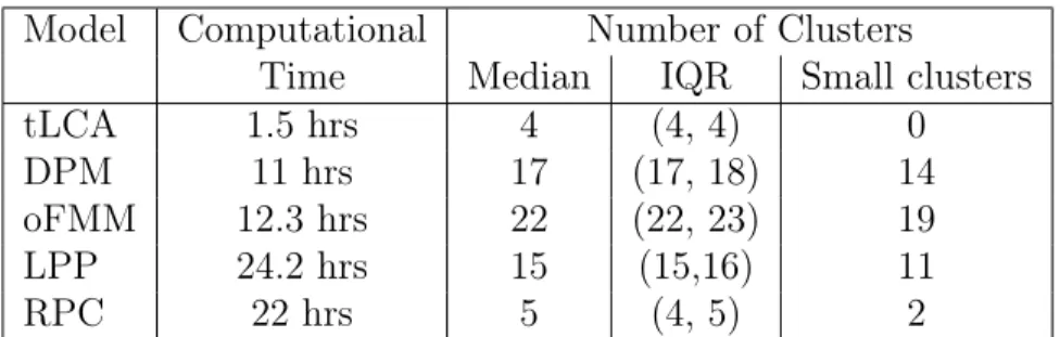
Model Computational Number of Clusters
Time Median IQR Small clusters
tLCA 1.5 hrs 4 (4, 4) 0
DPM 11 hrs 17 (17, 18) 14
oFMM 12.3 hrs 22 (22, 23) 19
LPP 24.2 hrs 15 (15,16) 11
RPC 22 hrs 5 (4, 5) 2
Table 3.1: Simulation results of models. A small cluster is defined as any cluster containing less than 5% of the population size
3.4.1 Results
All models were run using MATLAB 2017a. Examination of trace plots indicated quick convergence of model parameters. Comparison of model performance is summa-rized in Table 3.1. The tLCA had the shortest computational run time. The LPP and RPC had the longest computation run times. TheRPC showed considerable sparseness in deriving the number of global nonempty clusters with a median of 5 compared to the other models. The DPM and oFMM derived an excess number of nonempty global clusters. The LPP derived a median of 15 nonempty clusters and tLCA filled all four of its predefined clusters.
resembled subpopulations that contained highly deviant cluster patterns. The extrane-ousRPC models strongly resembled the two subpopulations that contained completely local cluster patterns. The extraneous cluster from tLCA had a weak concordance to all possible global or local patterns.
3.5 Analysis of National Birth Defects Prevention Study Data
3.5.1 Multivariate Categorical Dietary Data
The National Birth Defects Prevention Study is an ongoing multi-state population-based, case-control study of birth defects in the United States (Yoon et al. 2001). Infants were identified via birth defect surveillance in Arkansas, California, Iowa, Mas-sachusetts, New Jersey, New York, Texas, Georgia, North Carolina, and Utah. We focus in this analysis on dietary habits of control participants. Participants for this study included mothers with expected due dates from 1997 to 2009, totaling 9747 con-trols. Controls were defined as any live-born infant without any birth defects and were randomly selected from birth certificates or hospital records. Following prior analyses, subjects were excluded who had multiple births, a prior history of birth defects, preex-isting diabetes, or folate antagonist medication use from three months before pregnancy to the end of pregnancy. In accordance with NBDPS standard practices, mothers with daily energy intake below the 2.5th and above the 97.5th percentiles were also excluded to prevent inclusion of unlikely intake data. After exclusion criteria were applied, a total of 9010 controls were included for this analysis.
an individual food item consumed over the total food items consumed, using grams per day as the consumption metric. Grams per day of a food item was determined by multiplying the standard portion size listed on the FFQ and the self-reported frequency consumed. Distribution of food items showed a spike at zero, which is well known in the literature (Kipnis et al. 2009, Zhang et al. 2011). Keeping with common dietary analysis practices, these percentiles were aggregated into four relative consumption levels: no consumption, low consumption (0-33% consumed), medium consumption (33-66% consumed), and high consumption (66-100% consumed). A total of p = 63 food items were included in the study with four consumption levels (d = 4) fit into a categorical distribution.
Given the standard mixture model setup, where zik is the membership indicator of subject i to cluster k,
f(yi) = K X k=1 πk p Y j=1
f(yij|zik) = K X k=1 πk p Y j=1 d Y c=1
θ1(yij=c)
jc|k , (3.7)
where θjc|k represents the probability of a subject with consumption level c from food item j given allocation to dietary cluster k. We transition to the RPC model, where
θjc|k is split into two variables: θ0jc|k and θ(s)1jc|l. The former represents the probability of a subject having a consumption level of c from food item j, given allocation to
global dietary profile k. The latter representing the probability of a subject from
subpopulation s having a consumption level c from food item j given allocation to
local dietary cluster l. Similarly, zik would be split into Ci and Lij variables, where
Ci is the membership indicator of subject i for the global variables and Lij is the membership indicator of subject ifor deviated variable j.
The cluster-specific parameters were each drawn from a flat, symmetric Dirichlet dis-tribution, Θ0j·|h ={θ0j1|h, . . . , θ0jd|h} ∼ Dird(η), Θ
(s)
1j·|h ={θ (s)
1j1|h, . . . , θ (s)
where η = 1. The hyperparameters of the Beta-Bernoulli process component of the RPC were drawn from a gamma prior, β(s) ∼ Γ(1,1). To encourage a flat prior setup of the Beta-Bernoulli process, β(s) was set to 1 for simplicity.
3.5.2 MCMC Performance
As performed in simulation, sampling was performed with an MCMC run of 20,000 iterations, after a 5,000 burn-in. Given the tendency, acknowledged in the simulation study, of parameters gravitating to a preferred node and remaining there for subsequent iterations in large samples, the random permutation sampler was applied to encourage mixing (Frühwirth-Schnatter 2001). Furthermore, the overfitted model is also prone to generating extraneous and redundant clustering (van Havre et al. 2015). Redundancies were removed by creating a posterior pairwise comparison matrix based on the full MCMC output. Hierarchical clustering was then performed using the complete linkage approach, restricting to the median number of nonempty clusters larger than 5% in size (Krebs et al. 1989, Medvedovic and Sivaganesan 2002). This threshold was determined from the simulation study in order to focus on identifying the clusters of global interest. The trace plots of β(s) and π
1:K showed a good mixing and rapid convergence. All model parameters were estimated by calculating the posterior median and 95% credible intervals.
3.5.3 NBDPS Results
Figure 3.1: Heat map showing modal consumption level of RPC global profiles. Blue -no consumption, yellow - low consumption, orange - medium consumption, red - high consumption.
map illustrating the patterns of the global profiles is provided in Figure 3.1. Global profile behaviors were described by foods most likely to have a given consumption level within each cluster. Figure 3.2 illustrates the top five foods with the highest probability of having a given consumption level for each global profile. Note some foods were listed under multiple consumption levels. This demonstrates similar modalities for more than one consumption compared to the other foods. The greater of these modalities is reflected in the consumption map of Figure 3.1.
Figure 3.2: Top 5 foods most likely to be consumed at each level of global profiles
Texas had a strong representation of global profile 4 which had a high consumption of foods commonly found in a ‘Tex-Mex’ style diet (tortillas, refried beans, salsa).
Figure 3.3: Frequency distribution of global profiles by subpopulation (state) for the global profiles identified in the model
3.6 Discussion
The RPC method provides a convenient and informative population-based model that is able to adapt and account for potential deviations occurring within subpopula-tions. This was evident in the application of the NBDPS dietary data. Many precon-ceived notions of regional food trends were identified in this model. It calls attention to the overgeneralization of dietary practices in the United states as regionally indige-nous foods can sometimes be drivers of diet characterization. With an extension to case-control analysis, this method will be able to identify how deviations in a national or state diet can associate with various health outcomes.
Within each subpopulation, deviating items favored a heavier mass into a single cluster. This may be due to the relatively smaller sample size and more homogeneity that exists with a single subpopulation. Clustering at the global level removes infor-mation that is not pertinent to the overall population. That inforinfor-mation is subjugated to the subpopulation level where it can assume a separate local clustering of individual deviated variables. On occasion, some foods may share a local deviation in favor of non-consumption across all subpopulations. In this case, the global profile reflected the patterns of subjects that shared consumption behaviors with those from other subpop-ulations, while all non-consumers were localized to the state level.
CHAPTER 4: SUPERVISED ROBUST PROFILE CLUSTERING
4.1 Motivation
Robust profile clustering (RPC) is an exploratory technique that is able to dis-criminate features of a diverse population that contribute to the general population as opposed to a subpopulation. This is done by removing the overgeneralization of global clustering, where subjects can be clustered together but not assumed to respond to all exposures in a set identically. RPC provides a multilevel approach that allows subjects and variables to cluster both locally, within a subject’s respective subpopulation, and globally, across all subpopulations.
As an exploratory technique, RPC is able to identify features that are likely to trend over the general population compared to those localized within a subpopulation. Linking these derived clusters to an outcome requires an equally flexible regression model. Traditional regression models are limited due to the general assumption that a subject’s cluster assignment is consistent across all variables in the set. In the case of RPC, subjects can contain both global and local cluster assignments that differ from one variable to another. This means two subjects from different subpopulations could be in the same global cluster, but differ in variable deviation patterns. Similarly, two subjects from the same subpopulation could share deviation responses in variables, but belong to different global clusters.
to an outcome linked in aggregation. How subjects cluster is directly dependent on the association of the many exposures to that outcome.
We approach this concern by developing a predictive clustering model, that links the dual level clustering generated from the RPC with a response model. This allows subjects that are more likely to exhibit a health outcome to cluster in accordance with their combinatorial behavior profile. Similar ideas have been used to link functional predictors to various maternal health outcomes.
Dunson et al. used a predictor/response clustering model to determine the associ-ation of pregnancy weight gain with infant birth weight (Dunson et al. 2008). Simi-larly, Bigelow and Dunson (2009) created a predictive clustering model that used post-ovulatory progesterone data to predict early pregnancy loss. The results from these studies have shown promising results, but new methods are needed to accommodate multivariate categorical data in a nonparametric model.
We organize this chapter as follows. Section 2 introduces the supervised RPC joint model. Section 3 describes the algorithm for posterior computation and inference. Section 4 presents an application of the model using the NBDPS data to determine an association between maternal diet and oral cleft birth defects. We conclude with a short discussion on extensions and further methodological developments with the model in Section 5.
4.2 Supervised RPC Joint Model
4.2.1 Robust Profile Clustering Predictor Model
subjects in a general population that is comprised ofS subpopulations. Each
subpop-ulations ∈(1, . . . , S) contains ns subjects. Letxi = (xi1, . . . , xip) denote the observed data vector for subjecti for all p variables.
The global clustering component is generated from a finite mixture model, such that
P r(Ci =h) = πh, π= (π1, . . . , πK)∼Dir(K1, . . . ,K1), where K is the expected number of global clusters in the model. If the number of clusters is unknown, a conservative upper bound that far exceeds the expected number of clusters in the model can be used to mimic an overfitted finite mixture model (Rousseau and Mengersen 2011). The local clustering component may also be generated from an overfitted finite mixture model, for each subpopulationsand variablej ∈(1, . . . , p), whereP r(Lij =l|si =s) =λ
(s) h , λ
(s) = (λ(s)1 , . . . , λ(s)K) ∼Dir(K1, . . . ,K1). The global/local allocation component, Gij is drawn from a Beta-Bernoulli process, where Gij|si = s ∼ Bern(ν
(s) j ), ν
(s)
j ∼ B(1, β(s)), for each variablej ∈(1, . . . , p), and s denotes the corresponding subpopulation for subject i.
Let K0 denote the number of nonempty global clusters derived in the RPC model, and Ks the number of nonempty local clusters derived for subpopulation s. Each global and local cluster is represented with parameters Θ0 and Θ
(s)
f(xi|π, λ, Gij,Θ0,Θ1) = K0 X h=1 πh p Y
j:Gij=1
dj
Y
c=1
θ1(xij=c)
0jh,c
p Y
j:Gij=0
Ks
X
l=1
λ(s)l
dj
Y
c=1
θ1(xij=c)
1jl,c
(4.1)
4.2.2 Probit Regression Response Model
At each iteration in the MCMC algorithm, the current global cluster index, Ci,
assigned to each subject is added to the probit model as a fixed effect covariate, where
yi = 1, indicates an oral cleft birth defect outcome. While the global cluster assign-ment can change from iteration to iteration, all other predictors in the model remain fixed. We represent the set of subject-specific observed covariates as Wi. These
co-variates include study site location of the subject, designated by s and a collective
set of demographic variables, Wi ∈(age, race, BMI, smoking, alcohol intake, maternal education).
P(yi = 1|Wi, Ci) = Φ
ξ1 + S X
s=2
1(si =s)ξs+ K0
X
k=2
1(Ci =k)ξS+h+Wiξdem
(4.2)
4.3 Methods
4.3.1 Parameter Estimation
The joint model is intended to estimate both parameters from the RPC-predictor model and the probit response model concurrently in an MCMC algorithm. Yet, when the number of global clusters is not knowna priori an overfitted finite mixture model is necessary to first determine the appropriate number of global clusters to fit in the joint model.
4.3.2 MCMC Algorithm
We set up the model with Ga(1,1) prior on the Beta-Bernoulli process hyperpa-rameter {β(s)}S
s=1. Assuming a multinomial categorical dataset where all variables contain ddifferent response levels, we select a flat symmetrical Dirichlet prior (η= 1), for Θ0j|h = {θ0jh,1, . . . , θ0jh,d} for all j ∈ (1, . . . , p) variables, in each global cluster
h ∈ (1, . . . , K), and likewise for the local cluster density parameters. Covariates in-cluded in the model were generated from the standard multivariate normal distribution. To encourage sparsity, the Dirichlet hyperparameter of the global and local finite mix-tures was selected asα= 10001 . Latent response variable,zi, was drawn from a truncated
normal distribution, based on if the subject was designated as an oral cleft defect case (yi = 1) or healthy control (yi = 0), as detailed below.
P(yi = 1|Wi, ξ, Ci) = Φ(Wi, ξ)
Zi =ξ1+ S X
s=2
1(si =s)ξs+ K0
X
k=2
1(Ci =k)ξS+h+Wiξdem+i
wherei ∼N(0,1)
Φ(Zi) =
>0, when yi = 1
≤0, whenyi = 0
(4.3)
coefficient cestimate at iteration t.
Posterior Computation and Inference
We propose a simple Gibbs sampler for posterior computation.
1. Update the global component indicators (Gij |si =s)∼Bern(pij), where
pij =
νj(s)Qdc=1Θ1(xij=c)
0jCi,c
νj(s)Qdc=1Θ1(xij=c)
0jCi,c + (1−ν
(s) j )
Qd c=1(Θ
(s) 1jLij,c)
1(xij=c)
for each subjecti∈(1, . . . , n) with respective subpopulation index s.
2. Update global cluster index Ci, i = 1, . . . , n from its multinomial distribution
where
P r(Ci =h) =
πh Q
j:Gij=1
Qd c=1Θ
1(xij=c)
0jh,c PK
l=1πl Q
j:Gij=1
Qd c=1Θ
1(xij=c)
0jl,c
.
3. Update local cluster index Lij for all i : si = s and j = 1, . . . , p, repeating for eachs, from its multinomial distribution conditional on si =s where
P r(Lij =h) =
λ(s)h Qdc=1Θ(s)1jh,c
1(xij=c,Gij=0)
PK l=1λ (s) l Qd c=1 Θ(s)1jl,c
1(xij=c,Gij=0).
4. Update the global clustering weights
π = (π1, . . . , πK)∼Dir α+ n X
i=1
1(Ci = 1), . . . , α+ n X
i=1
1(Ci =K) !
.
5. Update the local clustering weights in subpopulation s,
λ(s)=λ(s)1 , . . . , λ(s)K ∼Dir α+ X i:si=s
p X
j=1
1(Lij = 1), . . . , α+ X
i:si=s
p X
j=1
1(Lij =K) !
6. Update the multinomial parameters
Θ0jh ∼Dir
1 + X
i:Gij=1,Ci=h
1(yij = 1), . . . ,1 +
X
i:Gij=1,Ci=h
1(yij =d)
Θ(s)1jh ∼Dir
1 + X
i:Gij=0,Lij=h,si=s
1(yij = 1), . . . ,1 +
X
i:Gij=0,Lij=h,si=s
1(yij =d)
7. Update νj(s)∼Be(1 +P
i:si=sGij, β
(s)+P
i:si=s(1−Gij)).
8. Update Beta-Bernoulli hyperparameter: β(s) ∼Ga(a
β+p, bβ− Pp
j=1log(1−ν (s) j )). 9. Update regression coefficients: ξ∼M V N((Σ−10 +W0W)−1(Σ−10 µ0+W0Z),(Σ−10 +
W0W)−1).
10. Update latent response variable: Zi|ξ, yi ∼
Nzi≤0(Wiξ,1) when yi = 0
Nzi>0(Wiξ,1) when yi = 1
4.4 Application to National Birth Defects Prevention Study
4.4.1 NBDPS Dietary Data
North Carolina, Massachusetts). Two states only included data on live-born cases (New York, New Jersey). Exclusion criteria for this analysis included mothers with multiple births, a family history of clefts (33 controls, 224 cases), preexisting diabetes (109 con-trols, 86 cases), used folate antagonist medications(phenytoin, valproic acid, valproate sodium, carbamazepine, methotrexate, trimethoprim hydrochloride, trimethoprim sul-fate, trimethoprim, aminopterin sodium, phenobarbital, phenobarbital sodium, prim-idone, divalproex, and sodium) from the time period 3 months before pregnancy to the end of pregnancy (124 controls, 55 cases), reported extreme values in total caloric intake (<500 or> 5000 kcal) (314 controls, 125 cases), and missed more than 1 item in the food frequency questionnaire or data on folic acid/multi-vitamin supplement use (227 controls, 73 cases). After exclusions, a total of 3430 cases and 9010 controls were included for analysis.
4.4.2 Comparative Analysis
Deviance Information Criterion (DIC) was calculated for each model to evaluate model fitness of the supervised RPC joint model, compared to the traditional latent class model. The latent class model is a finite case. To determine the appropriate number of classes suitable for this data, models were fit with an increasing number of classes until best fit was reached. Post hoc testing revealed that the latent class model preferred 17 global classes. The deviance of the respective models were calculated using the product of both the clustering predictor model (4.1) and the probit response model (4.2). The latent class model’s log-likelihood function for the predictor model is outlined in (4.4).
logL(xi|π, θ) = N X i=1 log K X k=1 πk p Y j=1 dj Y c=1
θ1(xij=c)
jc|k
(4.4)
The DIC is calculated by taking the difference of the mean log-likelihood derived at each iteration of the MCMC with the log-likelihood derived using the posterior mean estimates of the model parameters, denotedθ˜(Spiegelhalter et al. 2002).
Figure 4.1: Heatmap showing modal cluster patterns of RPC global profiles. Legend: Blue-no consumption, Yellow-low consumption, Orange-medium consumption, Red-high consumption
at each consumption level for each global profile. Some foods were listed as top proba-bilities in more than one consumption level indicating similar modalities for that food. The greater of the two modal probabilities is reflected in its respective pattern of Figure 4.1. For example, global profile 1 has tortillas listed as a food most likely consumed at both the low and medium level. A reference to Figure 4.1, shows that for global profile 2, the modally favored consumption level for apples is medium. This is because the posterior probability of a subject in global profile 2 consuming apples with a relatively medium consumption level is 0.37, compared to a low consumption level probability of 0.29. In essence, most of the subjects allotted to global profile 2 will have a low or medium consumption with favor towards medium consumption.
Figure 4.2: Top 5 foods most likely to be consumed at each level of global profiles derived from RPC predictor model