Fast Solution of l 1 -norm Minimization Problems When the Solution May be Sparse

Fast Solution of

`

-norm Minimization Problems

When the Solution May be Sparse

David L. Donoho∗and Yaakov Tsaig† October 2006

Abstract

The minimum`1-norm solution to an underdetermined system of linear equationsy=Ax,

is often, remarkably, also the sparsest solution to that system. This sparsity-seeking property is of interest in signal processing and information transmission. However, general-purpose optimizers are much too slow for`1 minimization in many large-scale applications.

The Homotopy method was originally proposed by Osborne et al. for solving noisy overdetermined`1-penalized least squares problems. We here apply it to solve the noiseless

underdetermined `1-minimization problem min kxk1 subject to y = Ax. We show that

Homotopy runs much more rapidly than general-purpose LP solvers when sufficient sparsity is present. Indeed, the method often has the following k-step solution property: if the underlying solution has only k nonzeros, the Homotopy method reaches that solution in only k iterative steps. When this property holds andk is small compared to the problem size, this means that `1 minimization problems withk-sparse solutions can be solved in a

fraction of the cost of solving one full-sized linear system.

We demonstrate this k-step solution property for two kinds of problem suites. First, incoherent matrices A, where off-diagonal entries of the Gram matrix AT_{A are all smaller}

than M. If y is a linear combination of at most k ≤ (M−1 _{+ 1)/2 columns of A, we}

show that Homotopy has thek-step solution property. Second, ensembles of d×nrandom matricesA. If A has iid Gaussian entries, then, when y is a linear combination of at most

k < d/(2 log(n))·(1−n) columns, withn >0 small, Homotopy again exhibits thek-step

solution property with high probability. Further, we give evidence showing that for ensembles ofd×npartial orthogonal matrices, including partial Fourier matrices, and partial Hadamard matrices, with high probability, thek-step solution property holds up to a dramatically higher thresholdk, satisfyingk/d <ρˆ(d/n), for a certain empirically-determined function ˆρ(δ).

Our results imply that Homotopy can efficiently solve some very ambitious large-scale problems arising in stylized applications of error-correcting codes, magnetic resonance imag-ing, and NMR spectroscopy. Our approach also sheds light on the evident parallelism in results on`1minimization and Orthogonal Matching Pursuit (OMP), and aids in explaining

the inherent relations between Homotopy, LARS, OMP, and Polytope Faces Pursuit.

Key Words and Phrases: LASSO. LARS. Homotopy Methods. Basis Pursuit. `1 min-imization. Orthogonal Matching Pursuit. Polytope Faces Pursuit. Sparse Representations. Underdetermined Systems of Linear Equations.

Acknowledgements. This work was supported in part by grants from NIH, ONR-MURI, and NSF DMS 00-77261, DMS 01-40698 (FRG) and DMS 05-05303. We thank Michael Lustig and Neal Bangerter of the Magnetic Resonance Systems Research Lab (MRSRL) at Stanford University for supplying us with 3-D MRI data for use in our examples. YT would like to thank Michael Saunders for helpful discussions and references.

∗

Department of Statistics, Stanford University, Stanford CA, 94305

†

1

Introduction

Recently, `1-norm minimization has attracted attention in the signal processing community

[9, 26, 20, 7, 5, 6, 8, 27, 31, 32, 44], as an effective technique for solving underdetermined

systems of linear equations, of the following form. A measurement vector y ∈Rd is generated

from an unknown signal of interestx0∈Rn by a linear transformation y=Ax0, with a known

matrixA of size d×n. An important factor in these applications is thatd < n, so the system

of equations y=Axis underdetermined. We solve the convex optimization problem

(P1) min

x kxk1 subject to y=Ax,

obtaining a vectorx1 which we consider an approximation to x0.

Applications of (P1) have been proposed in the context of time-frequency representation [9],

overcomplete signal representation [20, 26, 27, 31, 32], texture/geometry separation [48, 49], compressed sensing (CS) [14, 7, 56], rapid MR Imaging [37, 38], removal of impulsive noise [21], and decoding of error-correcting codes (ECC) [5, 44]. In such applications, the underlying

problem is to obtain a solution toy =Axwhich is as sparse as possible, in the sense of having

few nonzero entries. The above-cited literature shows that often, when the desired solution x0

is sufficiently sparse, (P1) delivers either x0 or a reasonable approximation.

Traditionally, the problem of finding sparse solutions has been catalogued as belonging to a

class of combinatorial optimization problems, whereas (P1) can be solved by linear programming,

and is thus dramatically more tractable in general. Nevertheless, general-purpose LP solvers

ultimately involve solution of ‘full’ n×nlinear systems, and require many applications of such

solvers, each application costing orderO(n3) flops.

Many of the interesting problems where (P1) has been contemplated are very large in scale.

For example, already 10 years ago, Basis Pursuit [9] tackled problems with d = 8,192 and

n = 262,144, and problem sizes approached currently [55, 7, 56, 38] are even larger. Such

large-scale problems are simply too large for general-purpose strategies to be used in routine processing.

1.1 Greedy Approaches

Many of the applications of (P1) can instead be attacked heuristically by fitting sparse models,

using greedy stepwise least squares. This approach is often called Matching Pursuit or

Orthogo-nal Matching Pursuit (Omp) [12] in the signal processing literature. Rather than minimizing an

objective function,Omp constructs a sparse solution to a given problem by iteratively building

up an approximation; the vector yis approximated as a linear combination of a few columns of

A, where the active set of columns to be used is built column by column, in a greedy fashion.

At each iteration a new column is added to the active set – the column that best correlates with the current residual.

AlthoughOmpis a heuristic method, in some cases it works marvelously. In particular, there

are examples where the data y admit sparse synthesis using only k columns of A, and greedy

selection finds exactly those columns in just k steps. Perhaps surprisingly, optimists can cite

theoretical work supporting this notion; work by Troppet al. [52, 54] and Donohoet al. [19] has

shown that Omp can, in certain circumstances, succeed at finding the sparsest solution. Yet,

theory provides comfort for pessimists too; Omp fails to find the sparsest solution in certain

scenarios where `1 minimization succeeds [9, 15, 52].

Optimists can also rely on empirical evidence to support their hopeful attitude. By now

iid Gaussian elements and x0 is sparse but random (we are aware of experiments by Tropp,

by Petukhov, as well as ourselves) all with the conclusion that Omp – despite its greedy and

heuristic nature – performs roughly as well as (P1) in certain problem settings. Later in this

paper we document this in detail. However, to our knowledge, there is no theoretical basis supporting these empirical observations.

This has the air of mystery – why do (P1) and Omp behave so similarly, when one has a

rigorous foundation and the other one apparently does not? Is there some deeper connection

or similarity between the two ideas? If there is a similarity, why is Omp so fast while `1

minimization is so slow?

In this paper we aim to shed light on all these questions.

1.2 A Continuation Algorithm To Solve (P1)

In parallel with developments in the signal processing literature, there has also been interest in

the statistical community in fitting regression models while imposing`1-norm constraints on the

regression coefficients. Tibshirani [51] proposed the so-called Lasso problem, which we state

using our notation as follows:

(Lq) min

x ky−Axk

2

2 subject to kxk1 ≤q;

in words: a least-squares fit subject to an`1-norm constraint on the coefficients. In Tibshirani’s

original proposal,Ad×n was assumed to have d > n, i.e. representing an overdetermined linear

system.

It is convenient to consider instead the unconstrained optimization problem

(Dλ) min

x ky−Axk

2

2/2 +λkxk1,

i.e. a form of `1-penalized least-squares. Indeed, problems (Lq) and (Dλ) are equivalent under

an appropriate correspondence of parameters. To see that, associate with each problem (Dλ) :

λ∈ [0,∞) a solution ˜xλ (for simplicity assumed unique). The set {x˜λ : λ∈ [0,∞)} identifies

a solution path, with ˜xλ = 0 for λ large and, as λ→ 0, ˜xλ converging to the solution of (P1).

Similarly, {x˜q :q ∈ [0,∞)} traces out a solution path for problem (Lq), with ˜xq = 0 for q = 0

and, as q increases, ˜xq converging to the solution of (P1). Thus, there is a reparametrization

q(λ) defined by q(λ) =kx˜λk1 so that the solution paths of (Dλ) and (Lq(λ)) coincide.

In the classic overdetermined setting, d > n, Osborne, Presnell and Turlach [40, 41] made

the useful observation that the solution path of (Dλ), λ ≥ 0 (or (Lq), q ≥ 0) is polygonal.

Further, they characterized the changes in the solution ˜xλ at vertices of the polygonal path.

Vertices on this solution path correspond to solution subset models, i.e. vectors having nonzero elements only on a subset of the potential candidate entries. As we move along the solution

path, the subset is piecewise constant as a function of λ, changing only at critical values of λ,

corresponding to the vertices on the polygonal path. This evolving subset is called the active

set. Based on these observations, they presented the Homotopyalgorithm, which follows the

solution path by jumping from vertex to vertex of this polygonal path. It starts at ˜xλ= 0 for λ

large, with an empty active set. At each vertex, the active set is updated through the addition and removal of variables. Thus, in a sequence of steps, it successively obtains the solutions ˜

xλ` at a special problem-dependent sequence λ` associated to vertices of the polygonal path.

The name Homotopy refers to the fact that the objective function for (Dλ) is undergoing a

Malioutovet al. [39] were the first to apply theHomotopymethod to the formulation (Dλ)

in the underdetermined setting, when the data are noisy. In this paper, we also suggest using

theHomotopymethod for solving (P1) in the underdetermined setting.

Homotopy Algorithm for Solving(P1): Apply theHomotopymethod: follow the solution

path from xλ0 = 0 tox˜0. Upon reaching the λ= 0 limit, (P1)is solved.

Traditionally, to solve (P1), one would apply the simplex algorithm or an interior-point

method, which, in general, starts out with a dense solution and converges to the solution of (P1)

through a sequence of iterations, each requiring the solution of a full linear system. In contrast,

theHomotopymethod starts out atxλ0 = 0, and successively builds a sparse solution by adding

or removing elements from its active set. Clearly, in a sparse setting, this latter approach is

much more favorable, since, as long as the solution has few nonzeros,Homotopywill reach the

solution in a few steps.

Numerically, each step of the algorithm involves the rank-one update of a linear system,

and so if the whole procedure stops in k steps, yielding a solution with k nonzeros, its overall

complexity is bounded by k3+kdn flops. For kdand d∝n, this is far better than thed3/3

flops it would take to solve just one d×dlinear system. Moreover, to solve (Dλ) for all λ≥0

by a traditional approach, one would need to repeatedly solve a quadratic program for every λ

value of interest. For any problem size beyond the very smallest, that would be prohibitively

time consuming. In contrast,Homotopydelivers all the solutions ˜xλ to (Dλ), λ≥0.

1.3 LARS

Efron, Hastie, Johnstone, and Tibshirani [24] developed an approximation to the Homotopy

algorithm which is quite instructive. The Homotopy algorithm maintains an active set of

nonzero variables composing the current solution. When moving to a new vertex of the solution polygon, the algorithm may either add new elements to or remove existing elements from the

active set. The Lars procedure is obtained by following the same sequence of steps, only

omitting the step that considers removal of variables from the active set, thus constraining its behavior to adding new elements to the current approximation. In other words, once activated, a variable is never removed.

In modifying the stepwise rule, of course, one implicitly obtains a new polygonal path, the

Larspath, which in general may be different from theLassopath. Yet, Efron et al. observed

that in practice, the Lars path is often identical to the Lasso path. This equality is very

interesting in the present context, becauseLarsis so similar toOmp. Both algorithms build up

a model a step at a time, adding a new variable to the active set at each step, and ensuring that the new variable is in some sense the most important among the potential candidate variables. The details of determining importance differ but in both cases involve the inner product between the candidate new variables and the current residual.

In short, a stepwise algorithm with a greedy flavor can sometimes produce the same result

as full-blown`1 minimization. This suggests a possibility which can be stated in two different

ways:

• ... that an algorithm for quasi`1 minimization runs just as rapidly asOmp.

1.4 Properties of Homotopy

Another possibility comes to mind. The Homotopy algorithm is, algorithmically speaking,

a variant of Lars, differing only in a few lines of code. And yet this small variation makes

Homotopyrigorously able to solve a global optimization problem.

More explicitly, the difference between Homotopyand Lars lies in the provision by

Ho-motopyfor terms to leave as well as enter the active set. This means that the number of steps

required byHomotopy can, in principle, be significantly greater than the number of steps

re-quired byLars, as terms enter and leave the active set numerous times. If so, we observe “model

churning” which causes Homotopy to run slowly. We present evidence that under favorable

conditions, such churning does not occur. In such cases, the Homotopy algorithm is roughly

as fast as bothLarsand Omp.

In this paper, we consider two settings for performance measurement: deterministic

incoher-ent matrices and random matrices. We demonstrate that, when ak-sparse representation exists,

k d, the Homotopy algorithm finds it in k steps. Results in each setting parallel existing

results about Omp in that setting. Moreover, the discussion above indicates that each step of

Homotopyis identical to a step ofLarsand therefore very similar to a corresponding step of

Omp. We interpret this parallelism as follows.

The Homotopy algorithm, in addition to solving the `1 minimization problem,

runs just as rapidly as the heuristic algorithmsOmp/ Lars, in those problem suites

where those algorithms have been shown to correctly solve the sparse representation problem.

Since there exists a wide range of cases where `1-minimization is known to find the sparsest

solution whileOmpis known to fail [9, 15, 52],Homotopygives in some sense the best of both

worlds by a single algorithm: speed where possible, sparsity where possible.

In addition, our viewpoint sheds new perspective on previously-observed similarities between

results about`1 minimization and aboutOmp. Previous theoretical work [19, 52, 54] found that

these two seemingly disparate methods had comparable theoretical results for finding sparse solutions. Our work exhibits inherent similarities between the two methods which motivate these parallel findings.

Figure 1 summarizes the relation between`1 minimization andOmp, by highlighting the

inti-mate bonds betweenHomotopy,Lars, andOmp. We elaborate on these inherent connections

in a later section.

1.5 Main Results

Our results about the stopping behavior of Homotopyrequire some terminology.

Definition 1 A problem suite S(E,V;d, n, k) is a collection of problems defined by three

com-ponents: (a) an ensemble E of matrices Aof size d×n; (b) an ensemble V of n-vectorsα0 with

at mostk nonzeros; (c) an induced ensemble of left-hand sides y=Aα0.

Where the ensemble V is omitted from the definition of a problem suite, we interpret that as saying that the relevant statements hold for any nonzero distribution. Otherwise, V will take

one of three values: (Uniform), when the nonzeros are iid uniform on [0,1]; (Gauss), when the

nonzeros are iid standard normal; and (Bernoulli), when the nonzeros are iid equi-probable

!

l1 minimization

HOMOTOPY LARS

OMP

(1) (2) (3)

Figure 1: Bridging`1 minimization and OMP. (1)Homotopyprovably solves`1 minimization

problems [24]. (2)Larsis obtained fromHomotopyby removing the sign constraint check. (3)

OmpandLarsare similar in structure, the only difference being thatOmpsolves a least-squares

problem at each iteration, whereasLarssolves a linearly-penalized least-squares problem. There

are initially surprising similarities of results concerning the ability of OMP and`1 minimization

to find sparse solutions. We view those results as statements about thek-step solution property.

We present evidence showing that for sufficiently small k, steps(2) and (3) do not affect the

threshold for the k-sparse solution property. Since both algorithms have the k-step solution

property under the given conditions, they both have the sparse solution property under those conditions.

Definition 2 An algorithmAhas thek-step solution propertyat a given problem instance(A, y)

drawn from a problem suite S(E,V;d, n, k) if, when applied to the data (A, y), the algorithm

terminates after at most k steps with the correct solution.

Our main results establish thek-step solution property in specific problem suites.

1.5.1 Incoherent Systems

The mutual coherenceM(A) of a matrix Awhose columns are normalized to unit length is the

maximal off-diagonal entry of the Gram matrixATA. We call the collection of matrices Awith

M(A)≤µtheincoherent ensemblewith coherence boundµ(denotedIncµ). LetS(Incµ;d, n, k)

be the suite of problems with d×n matrices drawn from the incoherent ensemble Incµ, with

vectors α0 havingkα0k0 ≤k. For the incoherent problem suite, we have the following result:

Theorem 1 Let (A, y) be a problem instance drawn from S(Incµ;d, n, k). Suppose that

k≤(µ−1+ 1)/2. (1.1)

Then, the Homotopyalgorithm runs k steps and stops, delivering the solutionα0.

The condition (1.1) has appeared elsewhere; work by Donoho et al. [20, 18], Gribonval and

Nielsen [31], and Tropp [52] established that when (1.1) holds, the sparsest solution is unique

and equal to α0, and both`1 minimization and Omp recover α0. In particular, Omp takes at

mostksteps to reach the solution.

In short we show here that for the general class of problemsS(Incµ;d, n, k), where a unique

same solution in the same number of steps. Note thatHomotopyalways solves the`1 minimiza-tion problem; the result shows that it operates particularly rapidly over the sparse incoherent suite.

1.5.2 Random Matrices

We first considerd×nrandom matrices A from theUniform Spherical Ensemble (USE). Such

matrices have columns independently and uniformly distributed on the sphere Sd−1. Consider

the suiteS(USE;d, n, k) of random problems whereAis drawn from the USE and whereα0 has

at mostknonzeros at krandomly-chosen sites, with the sites chosen independently of A.

Empirical Finding 1 Fix δ ∈ (0,1). Let d = dn = bδnc. Let (A, y) be a problem instance

drawn fromS(USE;d, n, k). There is n>0 small, so that, with high probability, for

k≤ dn

2 log(n)(1−n), (1.2)

the Homotopy algorithm runsk steps and stops, delivering the solution α0.

Remarks:

• We conjecture that corresponding to this empirical finding is a theorem, in which the

conclusion is that asn→ ∞,n→0.

• The empirical result is in fact stronger. We demonstrate that for problem instances with

kemphatically not satisfying (1.2), but rather

k≥ dn

2 log(n)(1 +n),

then, with high probability for large n, the Homotopyalgorithm fails to terminate in k

steps. Thus, (1.2) delineates a boundary between two regions in (k, d, n) space; one where

the k-step property holds with high probability, and another where the chance of k-step

termination is very low.

• This empirical finding also holds for matrices drawn from the Random Signs Ensemble

(RSE). Matrices in this ensemble are constrained to have their entries ±1 (suitably

nor-malized to obtain unit-norm columns), with signs drawn independently and with equal probability.

We next consider ensembles made of partial orthogonal transformations. In particular, we

consider the following matrix ensembles:

• Partial Fourier Ensemble (PFE). Matrices in this ensemble are obtained by sampling at

randomdrows of annby nFourier matrix.

• Partial Hadamard Ensemble (PHE). Matrices in this ensemble are obtained by sampling

at randomdrows of annby nHadamard matrix.

• Uniform Random Projection Ensemble (URPE). Matrices in this ensemble are obtained

As it turns out, when applied to problems drawn from these ensembles, the Homotopy

al-gorithm maintains the k-step property at a substantially greater range of signal sparsities. In

detail, we give evidence supporting the following conclusion.

Empirical Finding 2 Fix δ ∈ (0,1). Let d = dn = bδnc. Let (A, y) be a problem instance

drawn fromS(E,V;d, n, k), with E∈ {PFE,PHE,URPE}, and V∈ {Uniform,Gauss,Bernoulli

}. The empirical function ρˆ(δ) depicted in Figure 8, marks a transition such that, for k/dn ≤

ˆ

ρ(δ), the Homotopyalgorithm runs k steps and stops, delivering the solution α0.

A third, and equally important, finding we present involves the behavior of the Homotopy

algorithm when thek-step property does not hold. We provide evidence to the following.

Empirical Finding 3 Let(A, y) be a problem instance drawn fromS(E,V;d, n, k), with E∈ {

PFE,PHE,URPE }, V ∈ { _{Uniform,Gauss,Bernoulli} }, and (d, n, k) chosen so that the k

-step property does not hold. With high probability,Homotopy, when applied to(A, y), operates

in either of two modes:

1. It recovers the sparse solutionα0 incs·diterations, with csa constant depending on E, V,

empirically found to be less than 1.6.

2. It does not recover α0, returning a solution to (P1) in cf ·diterations, with cf a constant

depending onE, V, empirically found to be less than4.85.

We interpret this finding as saying that we may safely apply Homotopy to problems whose

solutions are not knowna priorito be sparse, and still obtain a solution rapidly. In addition, if

the underlying solution to the problem is indeed sparse, Homotopyis particularly efficient in

finding it. This finding is of great usefulness in practical applications ofHomotopy.

1.6 An Illustration: Error Correction in a Sparse Noisy Channel

The results presented above have far-reaching implications in practical scenarios. We demon-strate these with a stylized problem inspired by digital communication systems, of correcting

gross errors in a digital transmission. Recently, researchers pointed out that`1-minimization/sparsity

ideas have a role to play in decoding linear error-correcting codes over Z [5, 44], a problem

known, in general, to be NP-hard. Applying theHomotopyalgorithm in this scenario, we now

demonstrate the following remarkable property, an implication of Empirical Finding 2.

Corollary 1 Consider a communications channel corrupting a fraction < 0.24 of every n

transmitted integers, the corrupted sites chosen by a Bernoulli() iid selection. For large n,

there exists a rate-1/5 code, that, with high probability, can be decoded, without error, in at most

.24n Homotopysteps.

In other words, even when as many as a quarter of the transmitted entries are corrupted,

Homotopy operates at peak performance, recovering the encoded bits in a fixed number of

steps, known in advance. This feature enables the design of real-time decoders obeying a hard computational budget constraint, with a fixed number of flops per decoding effort.

Let us describe the coding strategy in more detail. Assume θ is a digital signal of length

p, with entries ±1, representing bits to be transmitted over a digital communication channel.

Prior to transmission, we encode θ with a rate 1/5 code constructed in the following manner.

0.1 0.2 0.3 0.4 0.05

0.1 0.15 0.2 0.25 0.3 0.35

ε

# iterations / n

(a) Gaussian noise

0.1 0.2 0.3 0.4

0.05 0.1 0.15 0.2 0.25 0.3 0.35

ε

# iterations / n

(b) Bernoulli noise

0.1 0.2 0.3 0.4

0.05 0.1 0.15 0.2 0.25 0.3 0.35

ε

# iterations / n

(c) Cauchy noise

0.1 0.2 0.3 0.4

0.05 0.1 0.15 0.2 0.25 0.3 0.35

ε

# iterations / n

(d) Rayleigh noise

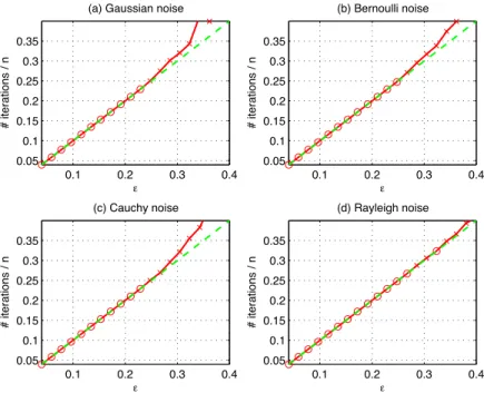
Figure 2: Performance of Homotopy in decoding a rate-1/5 partial Hadamard code. Each

panel shows the number of iterations, divided byn, that Homotopy takes in order to recover

the coded signal, versus , the fraction of corrupt entries in the transmitted signal, with the

noise distributed (a) N(0,1); (b)±1 with equal probabilities; (c) Cauchy; (d) Rayleigh. In each

plot ‘o’ indicates k-step recovery, and ‘x’ implies recovery in more thanksteps.

p rows of H at random. The ‘decoding matrix’ D is then composed of the other 4p rows of H.

The encoding stage amounts to computingx=ETθ, withx the encoded signal, of lengthn. At

the decoder, we receiver =x+z, wherez has nonzeros inkrandom positions, and the nonzero

follow a specified distribution. At the decoder, we applyHomotopyto solve

(EC1) minkαk1 subject to Dα=Dr;

Call the solution ˆα. The decoder output is then

ˆ

θ= sgn(ET(r−αˆ)).

The key property being exploited is the mutual orthogonality of D and E. Specifically, note

thatDr =D(ETθ+z) =Dz. Hence, (EC1) is essentially solving for the sparse error patten.

To demonstrate our claim, we setp= 256, and considered error ratesk=n, with varying

in [0.04,0.4]. In each case we generated a problem instance as described above, and measured the

number of steps Homotopytakes to reach the correct solution. Results are plotted in Figure

2, showing four different noise distributions. Inspecting the results, we make two important observations. First, as claimed, for the noise distributions considered, as long as the fraction

of corrupt entries is less that 0.24n, Homotopy recovers the correct solution in k steps, as

implied by Empirical Finding 2. Second, as increases, the k-step property may begin to fail,

butHomotopystill does not take many more than k steps, in accord with Empirical Finding

1.7 Relation to Earlier Work

Our results seem interesting in light of previous work by Osborne et al. [40] and Efron et

al. [24]. In particular, our proposal for fast solution of `1 minimization amounts simply to

applying to (P1) previously known algorithms (Homotopy a.k.a Lars/Lasso) designed for

fitting equations to noisy data. We make the following contributions.

• Few Steps. Efron et al. considered the overdetermined noisy setting, and remarked in

passing that while, in principle Homotopycould take many steps, they had encountered

examples where it took a direct path to the solution, in which a term, once entered into the active set, stayed in the active set [24]. Our work in the noiseless underdetermined

setting formally identifies a precise phenomenon, namely, thek-step solution property, and

delineates a range of problem suites where this phenomenon occurs.

• Similarity of Homotopy and Lars. Efron et al., in the overdetermined noisy setting,

commented that, while in principle the solution paths ofHomotopyand Lars could be

different, in practice they were came across examples whereHomotopyandLarsyielded

very similar results [24]. Our work in the noiseless case formally defines a property which

implies that Homotopy and Larshave the same solution path, and delineates a range

of problem suites where this property holds. In addition, we present simulation studies

showing that, over a region in parameter space, where`1minimization recovers the sparsest

solution,Larsalso recovers the sparsest solution.

• Similarity of Homotopyand Omp. In the random setting, a result of Tropp and Gilbert

[54] as saying thatOmp recovers the sparsest solution under a condition similar to (1.2),

although with a somewhat worse constant term; their result (and proof) can be interpreted

in the light of our work as saying thatOmpactually has thek-step solution property under

their condition.

In fact it has thek-step solution property under the condition (1.2). Below, we elaborate

on the connections betweenHomotopyand Omp leading to these similar results.

• Similarity of Homotopy and Polytope Faces Pursuit. Recently, Plumbley introduced a

greedy algorithm to solve (P1) in the dual space, which he namedPolytope Faces Pursuit

(Pfp) [43, 42]. The algorithm bears strong resemblance to Homotopyand Omp. Below,

we elaborate on Plumbley’s work, to show that the affinities are not coincidental, and

in fact, under certain conditions, Pfp is equivalent to Homotopy. We then conclude

that Pfp maintains the k-step solution property under the same conditions required for

Homotopy.

In short, we provide theoretical underpinnings, formal structure, and empirical findings. We

also believe our viewpoint clarifies the connections between Homotopy,Lars, and Pfp.

1.8 Contents

The paper is organized as follows. Section 2 reviews theHomotopyalgorithm in detail. Section

3 presents running-time simulations alongside a formal complexity analysis of the algorithm, and

discusses evidence leading to Empirical Finding 3. In Section 4 we prove Theorem 1, thek-step

solution property for the sparse incoherent problem suite. In Section 5 we demonstrate Empirical

Finding 1, thek-step solution property for the sparse USE problem suite. Section 6 follows, with

minimization andOmphinted at in Figure 1. This provides a natural segue to Section 8, which

discusses the connections between Homotopyand Pfp. Section 9 then offers a comparison of

the performance ofHomotopy,Lars,Omp andPfpin recovering sparse solutions. In Section

10, we demonstrate the applicability ofHomotopyand Larswith examples inspired by NMR

spectroscopy and MR imaging. Section 11 discusses the software accompanying this paper. Section 12 briefly discusses approximate methods for recovery of sparse solutions, and a final section has concluding remarks.

2

The Homotopy Algorithm

We shall start our exposition with a description of theHomotopy algorithm. Recall that the

general principle undergirding homotopy methods is to trace a solution path, parametrized by one or more variables, while evolving the parameter vector from an initial value, for which the

corresponding solution is known, to the desired value. For theLassoproblem (Dλ), this implies

following the solution xλ, starting at λlarge andxλ = 0, and terminating when λ→ 0 and xλ

converging to the solution of (P1). The solution path is followed by maintaining the optimality

conditions of (Dλ) at each point along the path.

Specifically, let fλ(x) denote the objective function of (Dλ). By classical ideas in convex

analysis, a necessary condition forxλ to be a minimizer of fλ(x) is that 0∈∂xfλ(xλ), i.e. the

zero vector is an element of the subdifferential of fλ atxλ. We calculate

∂xfλ(xλ) =−AT(y−Axλ) +λ∂kxλk1, (2.3)

where∂kxλk1 is the subgradient

∂kxλk1 =

u∈Rn

ui = sgn(xλ,i), xλ,i 6= 0

ui ∈[−1,1], xλ,i = 0

.

LetI ={i:xλ(i)6= 0}denote the support ofxλ, and callc=AT(y−Axλ) the vector ofresidual

correlations. Then, equation (2.3) can be written equivalently as the two conditions

c(I) =λ·sgn(xλ(I)), (2.4)

and

|c(Ic)| ≤λ, (2.5)

In words, residual correlations on the support I must all have magnitude equal to λ, and signs

that match the corresponding elements ofxλ, whereas residual correlations off the support must

have magnitude less than or equal toλ. TheHomotopyalgorithm now follows from these two

conditions, by tracing out the optimal pathxλ that maintains (2.4) and (2.5) for allλ≥0. The

key to its successful operation is that the path xλ is a piecewise linear path, with a discrete

number of vertices [24, 40].

The algorithm starts with an initial solution x0 = 0, and operates in an iterative fashion,

computing solution estimatesx`,`= 1,2, . . .. Throughout its operation, it maintains theactive

setI, which satisfies

I ={j:|c`(j)|=kc`k∞=λ}, (2.6)

as implied by conditions (2.4) and (2.5). At the`-th stage,Homotopyfirst computes an update

directiond`, by solving

withd`set to zero in coordinates not inI. This update direction ensures that the magnitudes of residual correlations on the active set all decline equally. The algorithm then computes the step size to the next breakpoint along the homotopy path. Two scenarios may lead to a breakpoint.

First, that a non-active element of c` would increase in magnitude beyond λ, violating (2.5).

This first occurs when

γ+_` = min

i∈Ic

λ−c`(i)

1−aT

i v`

,λ+c`(i)

1 +aT

i v`

, (2.8)

wherev` =AId`(I), and the minimum is taken only over positive arguments. Call the minimizing

index i+. The second scenario leading to a breakpoint in the path occurs when an active

coordinate crosses zero, violating the sign agreement in (2.4). This first occurs when

γ_`−= min

i∈I{−x`(i)/d`(i)}, (2.9)

where again the minimum is taken only over positive arguments. Call the minimizing indexi−.

Homotopythen marches to the next breakpoint, determined by

γ`= min{γ<sub>`</sub>+, γ_`−}, (2.10)

updates the active set, by either appendingI withi+, or removingi−, and computes a solution

estimate

x` =x`−1+γ`d`.

The algorithm terminates whenkc`k∞= 0, and the solution of (P1) has been reached.

Remarks:

1. In the algorithm description above, we implicitly assume that at each breakpoint on the homotopy path, at most one new coordinate is considered as candidate to enter the active

set (Efronet al. called this the “one at a time” condition [24]). If two or more vectors are

candidates, more care must be taken in order to choose the correct subset of coordinates to enter the active set; see [24] for a discussion.

2. In the introduction, we noted that theLarsscheme closely mimicsHomotopy, the main

difference being thatLarsdoes not allow removal of elements from the active set. Indeed,

to obtain theLars procedure, one simply follows the sequence of steps described above,

omitting the computation ofi− and γ_`−, and replacing (2.10) with

γ`=γ<sub>`</sub>+.

The resulting scheme adds a single element to the active set at each iteration, never removing active elements from the set.

3. The Homotopyalgorithm may be easily adapted to deal with noisy data. Assume that

rather than observingy0 =Aα0, we observe a noisy version y=Aα0+z, withkzk2≤n.

Donoho et al. [19, 16] have shown that, for certain matrix ensembles, the solution xq of

(Lq) withq =nhas an error which is at worst proportional to the noise level. To solve for

xn, we simply apply the Homotopy algorithm as described above, terminating as soon

as the residual satisfies kr`k ≤ n. Since in most practical scenarios it is not sensible to

assume that the measurements are perfectly noiseless, this attribute ofHomotopymakes

3

Computational Cost

In earlier sections, we claimed that Homotopy can solve the problem (P1) much faster than

general-purpose LP solvers, which are traditionally used to solve it. In particular, when the

k-step solution property holds, Homotopy runs in a fraction of the time it takes to solve one

full linear system, making it as efficient as fast stepwise algorithms such as Omp. To support

these assertions, we now present the results of running-time simulations, complemented by a

formal analysis of the asymptotic complexity of Homotopy.

3.1 Running Times

To evaluate the performance of the Homotopy algorithm applied to (P1), we compared its

running times on instances of the problem suite S(USE,Gauss;d, n, k) with two

state-of-the-art algorithms for solving Linear Programs. The first, LP Solve, is a Mixed Integer Linear Programming solver, implementing a variant of the Simplex algorithm [2]. The other, PDCO, a Primal-Dual Convex Optimization solver, is a log-barrier interior point method, written by Michael Saunders of the Stanford Optimization Laboratory [45]. Table 1 shows the running times

for Homotopy, LP Solve and PDCO, for various problem dimensions. The figures appearing

in the table were measured on a 3GHz Xeon workstation.

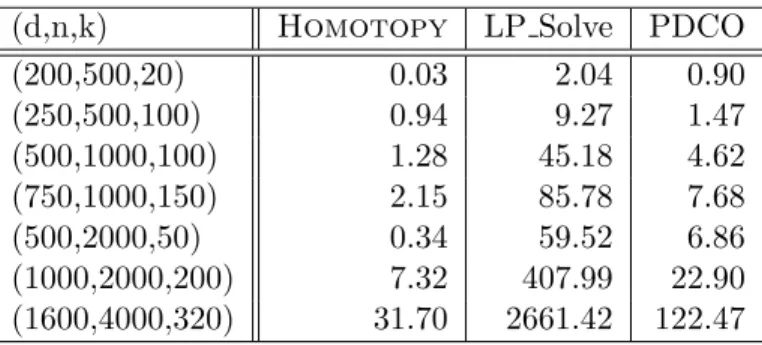
(d,n,k) Homotopy LP Solve PDCO

(200,500,20) 0.03 2.04 0.90

(250,500,100) 0.94 9.27 1.47

(500,1000,100) 1.28 45.18 4.62

(750,1000,150) 2.15 85.78 7.68

(500,2000,50) 0.34 59.52 6.86

(1000,2000,200) 7.32 407.99 22.90

(1600,4000,320) 31.70 2661.42 122.47

Table 1: Comparison of execution times (in seconds) of Homotopy, LP Solve and PDCO,

applied to instances of the random problem suiteS(USE,Gauss;d, n, k).

Examination of the running times in the table suggests two important observations. First,

when the underlying solution to the problem (P1) is sparse, a tremendous saving in computation

time is achieved usingHomotopy, compared to traditional LP solvers. For instance, when A

is 500×2000, and y admits sparse synthesis with k = 50 nonzeros, Homotopy terminates

in about 0.34 seconds, 20 times faster than PDCO, and over 150 times faster than LP Solve.

Second, when the linear system is highly underdetermined (i.e. d/n is small), even when the

solution is not sparse,Homotopy is more efficient than either LP Solve or PDCO. This latter

observation is of particular importance for applications, as it implies that Homotopy may be

‘safely’ used to solve`1 minimization problems even when the underlying solution is not known

to be sparse.

3.2 Complexity Analysis

The timing studies above are complemented by a detailed analysis of the complexity of the

Homotopy algorithm. We begin by noting that the bulk of computation is invested in the

solution of the linear system (2.7) at each iteration. Thus, the key to an efficient

addition/removal of elements to/from the active set. This allows for fast solution for the

up-date direction;O(d2) operations are needed to solve (2.7), rather than the O(d3) flops it would

ordinarily take. In detail, let ` = |I|, where I denotes the current active set. The dominant

calculations per iteration are the solution of (2.7) at a cost of 2`2 flops, and computation of the

step to the next vertex on the solution path, usingnd+ 6(n−`) flops. In addition, the Cholesky

factor of AT_IAI is either updated by appending a column to AI at a cost of `2+`d+ 2(`+d)

flops, or ‘downdated’ by removing a column ofAI using at most 3`2 flops.

To conclude, without any sparsity constraints on the data, k Homotopy steps would take

at most 4kd2/3 +kdn+O(kn) flops. However, if the conditions for the k-step solution property

are satisfied, a more favorable estimate holds.

Lemma 1 Let (A, y) be a problem instance drawn from a suite S(E,V;d, n, k). Suppose the k

-step solution property holds, and the Homotopyalgorithm performs k steps, each time adding

a single element into the active set. The algorithm terminates in k3 +kdn+ 1/2k2(d−1) +

n(8k+d+ 1) + 1/2k(5d−3)flops.

Notice that, forkd, the dominant term in the expression for the operation count iskdn, the

number of flops needed to carry out k matrix-vector multiplications. Thus, we may interpret

Lemma 1 as saying that, under such favorable conditions, the computational workload of

Ho-motopyis roughly proportional tok applications of ad×nmatrix. For comparison, applying

least-squares to solve the underdetermined linear system Ax = y would require 2d2_n−2d3_/3

operations [30]. Thus, forkd,Homotopyruns in a fraction of the time it takes to solve one

least-squares system.

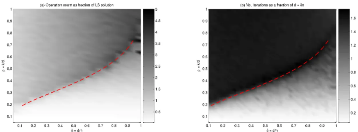
To visualize this statement, panel (a) of Figure 3 displays the operation count ofHomotopy

on a grid with varying sparsity and indeterminacy factors. In this simulation, we measured the

total operation count ofHomotopyas a fraction of the solution of oned×nleast-squares system,

for random instances of the problem suiteS(USE,Uniform;d, n, k). We fixedn= 1000, varied

the indeterminacy of the system, indexed by δ = d/n, in the range [0.1,1], and the sparsity

of the solution, indexed by ρ = k/d, in the range [0.05,1]. For reference, we superposed the

theoretical bound ρW below which the solution of (P1) is, with high probability, the sparsest

solution (see section 9 for more details). Close inspection of this plot reveals that, below this

curve, Homotopydelivers the solution to (P1) rapidly, much faster than it takes to solve one

d×n least-squares problem.

3.3 Number of Iterations

Considering the analysis just presented, it is clear that the computational efficiency of

Homo-topy greatly depends on the number of vertices on the polygonal Homotopy path. Indeed,

since it allows removal of elements from the active set, Homotopy may, conceivably, require

an arbitrarily large number of iterations to reach a solution. We note that this property is not

shared by Lars orOmp; owing to the fact that these algorithms never remove elements from

the active set, afterditerations they terminate with zero residual.

In [24], Efron et al. briefly noted that they had observed examples where Homotopydoes

not ‘drop’ elements from the active set very frequently, and so, overall, idoesn’t require many

more iterations than Lars to reach a solution. We explore this initial observation further,

and present evidence leading to Empirical Finding 3. Specifically, consider the problem suite S(E,V;d, n, k), with E ∈ {USE,PFE,PHE,URPE }, and V ∈ { Uniform,Gauss,Bernoulli

}. The space (d, n, k) of dimensions of underdetermined problems may be divided into three

Figure 3: Computational Cost ofHomotopy. Panel (a) shows the operation count as a fraction

of one least-squares solution on a ρ-δ grid, with n = 1000. Panel (b) shows the number of

iterations as a fraction ofd=δ·n. The superimposed dashed curve depicts the curveρW, below

which Homotopyrecovers the sparsest solution with high probability.

1. k-step region. When (d, n, k) are such that the k-step property holds, then Homotopy

successfully recovers the sparse solution ink steps, as suggested by Empirical Findings 1

and 2. Otherwise;

2. k-sparse region. When (d, n, k) are such that `1 minimization correctly recovers k-sparse

solutions but Homotopy takes more than k steps, then, with high probability, it takes

no more than cs·d steps, withcs a constant depending on E, V, empirically found to be

∼1.6. Otherwise;

3. Remainder. With high probability, Homotopy does not recover the sparsest solution,

returning a solution to (P1) incf·dsteps, withcf a constant depending onE, V, empirically

found to be∼4.85.

We note that the so-called “constants”cs, cf depend weakly on δ and n.

A graphical depiction of this division of the space of admissible (d, n, k) is given in panel

(b) of Figure 3. It shows the number of iterations Homotopy performed for various (d, n, k)

configurations, as a shaded attribute on a grid indexed by δ and ρ. Inspection of this plot

reveals that Homotopy performs at most ∼ 1.6·d iterations, regardless of the underlying

solution sparsity. In particular, in the region below the curveρW, where, with high probablity,

Homotopyrecovers the sparsest solution, it does so in less thandsteps.

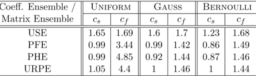
More extensive evidence is given in Table 2, summarizing the results of a comprehensive

study. We considered four matrix ensembles E, each coupled with three nonzero ensembles

V. For a problem instance drawn from a S(E,V;d, n, k), we recorded the number of iterations

required to reach a solution. We repeated this at many different (d, n, k) configurations,

gen-erating 100 independent realizations for each (d, n, k), and computing the average number of

iterations observed at each instance. Table 2 displays the estimated constantscs,cf for different

combinations of matrix ensemble and coefficient ensemble. Thus, the results in Table 2 read,

e.g., ‘Applied to a problem instance drawn from S(USE,Uniform;d, n, k), Homotopytakes,

Coeff. Ensemble / Uniform Gauss Bernoulli

Matrix Ensemble cs cf cs cf cs cf

USE 1.65 1.69 1.6 1.7 1.23 1.68

PFE 0.99 3.44 0.99 1.42 0.86 1.49

PHE 0.99 4.85 0.92 1.44 0.87 1.46

URPE 1.05 4.4 1 1.46 1 1.44

Table 2: Maximum number of Homotopy iterations, as a fraction of d, for various matrix /

coefficient ensembles.

4

Fast Solution with the Incoherent Ensemble

Let thed×nmatrixA have unit-length columnsaj,kajk2 = 1. The mutual coherence

M(A) = max

i6=j |hai, aji|

measures the smallest angle between any pair of columns. Asn > d, this angle must be greater

than zero: the columns cannot be mutually orthogonal; in fact, there is an established lower

bound on the coherence of A:

M(A)≥ s

n−d d(n−1),

Matrices which satisfy this lower bound with equality are known as optimal Grassmannian frames [50]. There is by now much work establishing relations between the sparsity of a coefficient vector

α0 and the coherence of a matrix A needed for successful recovery of α0 via `1 minimization

[20, 18, 53, 31] or Omp [19, 52]. In detail, for a general matrix A with coherence M(A), both

`1 minimization and OMP recover the solution α0 from datay=Aα0 whenever the number of

nonzeros inα0 satisfies

kα0k0<(M(A)−1+ 1)/2. (4.1)

see, for example, Theorem 7 of [18] or Corollary 3.6 of [52]. Comparing (4.1) with (1.1), we see

that Theorem 1 essentially states that a parallel result holds for theHomotopyalgorithm.

Before proceeding to the proof of the Theorem, we make a few introductory assumptions.

As in the above, we assume that the Homotopy algorithm operates with a problem instance

(A, y) as input, with y = Aα0 and kα0k0 =k. To simplify notation, we assume, without loss

of generality, that α0 has its nonzeros in the first k positions. Further, we operate under the

convention that at each step of the algorithm, only one vector is introduced into the active set. If two or more vectors are candidates to enter the active set, assume the algorithm inserts

them one at a time, on separate stages. Finally, to fix notation, let x` denote the Homotopy

solution at the `-th step, r` =y−Ax` denote the residual at that step, and c` =ATr` be the

corresponding residual correlation vector. To prove Theorem 1, we introduce two useful notions.

Definition 3 We say that the Homotopy algorithm has theCorrect Term Selection Property

at a given problem instance (A, y), with y = Aα0, if at each iteration, the algorithm selects a

new term to enter the active set from the support set of α0.

Homotopy has the correct term selection property if, throughout its operation, it builds the

solution using only correct terms. Thus, at termination, the support set of the solution is

Definition 4 We say that the Homotopy algorithm has the Sign Agreement Property at a

given problem instance (A, y), withy=Aα0, if at every step `, for allj∈I,

sgn(x`(j)) =sgn(c`(j)).

In words, Homotopy has the sign agreement property if, at every step of the algorithm, the

residual correlations in the active set agree in sign with the corresponding solution coefficients. This ensures that the algorithm never removes elements from the active set.

These two properties are the fundamental building blocks needed to ensure that the k

-step solution property holds. In particular, these two properties are necessary and sufficient

conditions for successful k-step termination, as the following lemma shows.

Lemma 2 Let(A, y)be a problem instance drawn from a suiteS(E,V;d, n, k). TheHomotopy

algorithm, when applied to(A, y), has thek-step solution property if and only if it has the correct

term selection property and the sign agreement property.

Proof. To argue in the forward direction, we note that, after k steps, correct term selection

implies that the active set is a subset of the support of α0, i.e. I ⊆ {1, ..., k}. In addition, the

sign agreement property ensures that no variables leave the active set. Therefore, afterksteps,

I ={1, ..., k}and theHomotopyalgorithm recovers the correct sparsity pattern. To show that

afterksteps, the algorithm terminates, we note that, at thek-th step, the step-sizeγkis chosen

so that, for somej∈Ic,

|ck(j)−γkaTjAIdk(I)|=λk−γk, (4.2)

withλk=kck(I)k∞. In addition, for the k-th update, we have

AIdk(I) =AI(ATIAI)−1ATIrk=rk,

sincerk is contained in the column space ofAI. Hence

ck(Ic) =ATIcA_Id_k(I),

and γk =λk is chosen to satisfy (4.2). Therefore, the solution at stepk has Axk =y. Since y

has a unique representation in terms of the columns of AI, we may conclude that xk=α0.

The converse is straightforward. In order to terminate with the solutionα0 afterksteps, the

Homotopy algorithm must select one term out of {1, ..., k} at each step, never removing any

elements. Thus, violation of either the correct term selection property or the sign agreement

property would result in a number of steps greater thankor an incorrect solution.

Below, we will show that, when the solution α0 is sufficiently sparse, both these properties

hold as the algorithm traces the solution path. Theorem 1 then follows naturally.

4.1 Correct Term Selection

We now show that, when sufficient sparsity is present, theHomotopysolution path maintains

the correct term selection property.

Lemma 3 Suppose that y=Aα0 where α0 has only knonzeros, with k satisfying

Assume that the residual at the `-th step can be written as a linear combination of the first k

columns in A, i.e.

r` = k X

j=1

β`(j)aj.

Then the next step of the Homotopyalgorithm selects an index from among the first k.

Proof. We will show that at the`-th step, max

1≤i≤k|hr`, aii|>maxi>k |hr`, aii|, (4.4)

and so at the end of the `-th iteration, the active set is a subset of{1, ..., k}.

Let G= ATA denote the gram matrix of A. Let ˆi= arg max1≤i≤k|βi|. The left hand side

of (4.4) is bounded below by max

1≤i≤k|hr`, aii| ≥ |hr`, aˆii| ≥ |

k X

j=1

β`(j)Gˆ<sub>ij</sub>| ≥ |β`(ˆi)| −

X

j6=ˆi

|Gˆij||β`(j)|

≥ |β`(ˆi)| −M(A) X

j6=ˆi |β`(j)|

≥ |β`(ˆi)| −M(A)(k−1)|β`(ˆi)|, (4.5)

Here we used: kajk22 = 1 for allj andGˆ_ij ≤M(A) forj 6= ˆi. As for the right hand side of (4.4),

we note that fori > k we have

|hr`, aii| ≤ k X

j=1

|β`(j)||Gij|

≤ M(A)

k X

j=1 |β`(j)|

≤ kM(A)|β`(ˆi)|. (4.6)

Combining (4.5) and (4.6), we get that for (4.4) to hold, we need

1−(k−1)M(A)> kM(A). (4.7)

Since kwas selected to exactly satisfy this bound, relation (4.4) follows.

Thus, when k satisfies (4.3), the Homotopy algorithm only ever considers indices among

the firstkas candidates to enter the active set.

4.2 Sign Agreement

Recall that an index is removed from the active set at step`only if condition (2.4) is violated, i.e.

if the signs of the residual correlations c`(i), i∈I do not match the signs of the corresponding

even stronger result holds: at each stage of the algorithm, the residual correlations in the active set agree in sign with the direction of change of the corresponding terms in the solution. In other words, the solution moves in the right direction at each step. In particular, it implies that

throughout the Homotopysolution path, the sign agreement property is maintained.

Lemma 4 Suppose that y=Aα0, where α0 has only knonzeros, with k satisfying

k≤(µ−1+ 1)/2.

For`∈ {1, ..., k}, letc`=ATr`, and let the active setI be defined as in (2.6). Then the update

directiond` defined by (2.7) satisfies,

sgn(d`(I)) =sgn(c`(I)). (4.8)

Proof. Letλ` =kc`k∞. We will show that fori∈I,|d`(i)−sgn(c`(i))|<1, implying that (4.8) holds. To do so, we note that (2.7) can be rewritten as

λ`(ATIAI−Id)d`(I) =−λ`d`(I) +c`(I),

whereId is the identity matrix of appropriate dimension. This yields

kλ`d`(I)−c`(I)k∞ ≤ kATIAI−Idk(∞,∞)· kλ`d`(I)k∞

≤ 1−M(A)

2 kλ`d`(I)k∞

≤ 1−M(A)

2 (kc`(I)k∞+kλ`d`(I)−c`(I)k∞)

≤ 1−M(A)

2 (λ`+kλ`d`(I)−c`(I)k∞),

wherek · k|_(∞,∞) denotes the induced`∞ operator norm. Rearranging terms, we get

kλ`d`(I)−c`(I)k∞≤λ`·

1−M

1 +M < λ`,

thus,

kd`(I)−sgn(c`(I))k∞<1.

Relation (4.8) follows.

4.3 Proof of Theorem 1

Lemmas 3 and 4 establish the correct term selection property and the sign agreement property at a single iteration of the algorithm. We will now give an inductive argument showing that the

two properties hold at every step`∈ {1, ..., k}.

In detail, the algorithm starts withx0 = 0; by the sparsity assumption ony=Aα0, we may

apply Lemma 3 withr0=y, to get that at the first step, a column among the firstkis selected.

Moreover, at the end of the first step we have x1 =γ1d1, and so, by Lemma 4,

sgn(x1(I)) =σ1(I).

By induction, assume that at step `, only indices among the first kare in the active set, i.e.

r` = k X

j=1

and the sign condition (2.4) holds, i.e.

sgn(x`(I)) =σ`(I).

Applying Lemma 3 tor`, we get that at the (l+ 1)-th step, the term to enter the active set will

be selected from among the first kindices. Moreover, for the updated solution we have

sgn(x`+1(I)) = sgn(x`(I) +γ`+1d`+1(I)).

By Lemma 4 we have

sgn(d`+1(I)) =σ`+1(I).

We observe that

c`+1 =c`−γ`+1ATAd`+1, whence, on the active set,

|c`+1(I)|=|c`(I)|(1−γ`+1), and so

σ`+1(I) =σ`(I).

In words, once a vector enters the active set, its residual correlation maintains the same sign. We conclude that

sgn(x`+1(I)) =σ`+1(I). (4.9)

Hence no variables leave the active set. To summarize, both the correct term selection property

and the sign agreement property are maintained throughout the execution of the Homotopy

algorithm.

We may now invoke Lemma 2 to conclude that the k-step solution property holds. This

completes the proof of Theorem 1.

5

Fast Solution with the Uniform Spherical Ensemble

Suppose now that A is a random matrix drawn from the Uniform Spherical Ensemble. It is

not hard to show that such matrices A are naturally incoherent; in fact, for > 0, with high

probability for large n

M(A)≤ r

4 log(n)

d ·(1 +).

Thus, applying Theorem 1, we get as an immediate corollary that if ksatisfies

k≤pd/log(n)·(1/4−0), (5.10)

then Homotopy is highly likely to recover any sparse vector α0 with at most k nonzeros.

However, as it turns out, Homotopyoperates much more efficiently when applied to instances

from the random suite S(USE;d, n, k), than what is implied by incoherence. We now discuss

evidence leading to Empirical Finding 1. We demonstrate, through a comprehensive suite of

simulations, that the formula d/(2 log(n)) accurately describes the breakdown of the k-step

solution property. Before doing so, we introduce two important tools that will be used repeatedly in the empirical analysis below.

5.1 Phase Diagrams and Phase Transitions

In statistical physics, aphase transitionis the transformation of a thermodynamic system from

one phase to another. The distinguishing characteristic of a phase transition is an abrupt

change in one or more of its physical properties, as underlying parameters cross a region of

parameter space. Borrowing terminology, we say that property P exhibits a phase transition

at a sequence of problem suites S(E,V;d, n, k), if there is a threshold function Thresh(d, n) on

the parameter space (k, d, n), such that problem instances withk≤Thresh(d, n) have property

P with high probability, and problem instances above this threshold do not have property P

with high probability. As we show below, the the k-step solution property of Homotopy,

applied to problem instances drawn fromS(USE;d, n, k), exhibits a phase transition at around

d/(2 log(n)). Thus, there is a sequence (n) with each term small and positive, so that for k <

(1−n)·d/(2 log(n)),Homotopydelivers the sparsest solution inksteps with high probability;

on the other hand, ifk >(1 +n)·d/(2 log(n)), then with high probablity,Homotopy, fails to

terminate in ksteps.

To visualize phase transitions, we utilize phase diagrams. In statistical physics, a phase

diagram is a graphical depiction of a parameter space decorated by boundaries of regions where certain properties hold. Here we use this term in an analogous fashion, to mean a graphical

depiction of a subset of the parameter space (d, n, k), illustrating the region where an algorithm

has a given property P, when applied to a problem suite S(E,V;d, n, k). It will typically take

the form of a 2-D grid, with the threshold function associated with the corresponding phase

transition dividing the grid into two regions: A region where property P occurs with high

probablity, and a region whereP occurs with low probablity.

While phase transitions are sometimes discovered by formal mathematical analysis, more commonly, the existence of phase transitions is unearthed by computer simulations. We now describe an objective framework for estimating phase transitions from simulation data. For

each problem instance (A, y) drawn from a suiteS(E,V;d, n, k), we associate a binary outcome

variable Y_kd,n, with Y_kd,n = 1 when property P is satisfied on that realization, and Y_kd,n =

0 otherwise. Within our framework, Y_kd,n is modeled as a Bernoulli random variable with

probabilityπ_kd,n. Thus,P(Y_kd,n= 1) =π_kd,n, andP(Y_kd,n= 0) = 1−π_kd,n. Our goal is to estimate

a value ˜kd,nwhere the transition between these two states occurs. To do so, we employ a logistic

regression model on the mean responseE{Y_kd,n}with predictor variable k,

E{Y_kd,n}= exp(β0+β1k)

1 + exp(β0+β1k)

. (5.11)

Logistic response functions are often used to model threshold phenomena in statistical data

analysis [34]. Let ˆπ_kd,ndenote the value of the fitted response function. We may then compute a

value ˆkd,nη indicating that, with probability exceeding 1−η, for a problem instance drawn from

S(E,V;d, n, k) withk <kˆd,nη , property P holds. ˆk is given by ˆ

π_kˆ= 1−η.

Thus, computing ˆkd,nη for a range of (d, n) values essentially maps out an empirical phase

tran-sitionof propertyP. The valueη fixes a location on the transition band below which we define

the region of success. In our work, we set η= 0.25.

5.2 The k-Step Solution Property

We now apply the method described in the previous section to estimate an empirical phase

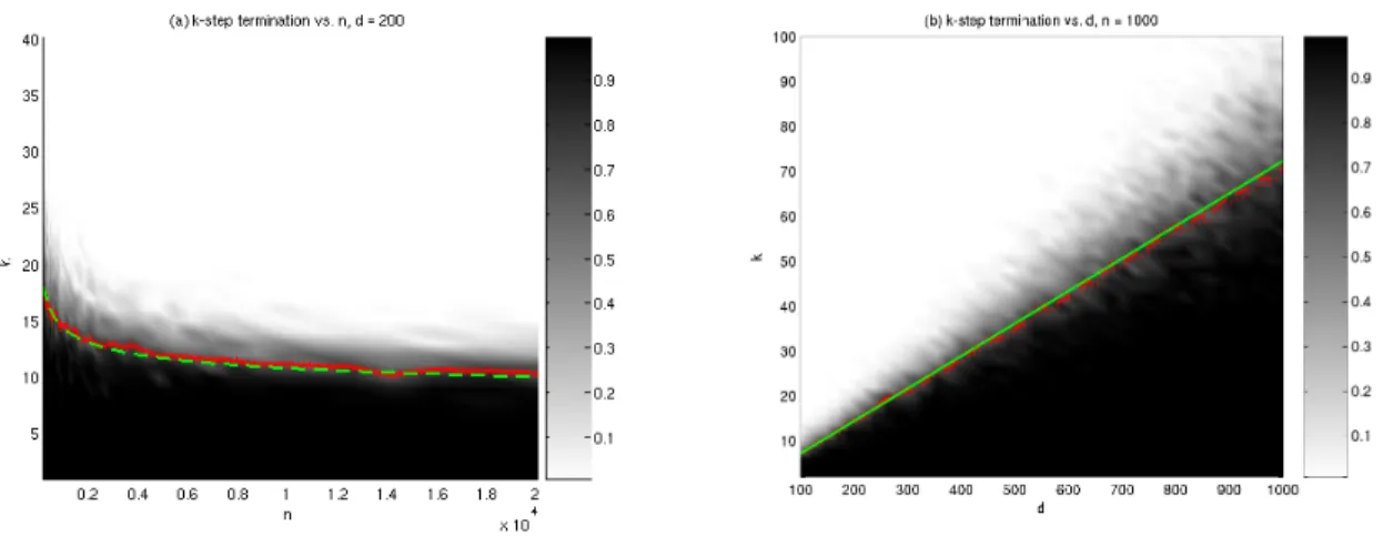
Figure 4: k-Step Solution Property of Homotopy for the Problem Suite

S(USE,Uniform;d, n, k). Shaded attribute is the proportion of successful terminations,

out of 100 trials, in the case: (a) k= 1. . .40,d= 200, andn= 200. . .20000; (b)k= 2. . .100,

d= 100. . .1000, and n= 1000. Overlaid are curves ford/(2 log(n)) (solid), ˆk₀d,n_.25 (dashed), and

the confidence bound for ˆk₀d,n_.25 with 95% confidence level (dotted).

briefly describe the experimental setup. For (d, n, k) given, we generated a problem instance

(A, y) drawn from the problem suite S(USE,Uniform;d, n, k). To this instance we applied the

Homotopy algorithm, and recorded the outcome of the response variable Y_kd,n. We did so in

two cases; first, fixing d= 200, varying nthrough 40 log-equispaced points in [200,20000] and

kthrough 40 equispaced points in [1,40]; second, keepingnfixed at 1000, varying dthrough 40

equispaced points in [100,1000] andkthrough 40 equispaced points in [2,100]. For each (d, n, k)

instance we ran 100 independent trials. To estimate the regression coefficients β0, β1 in (5.11),

we used maximum likelihood estimation [34].

Figure 4 displays two phase diagrams, giving a succinct depiction of the simulation results.

Panel (a) displays a grid of (k, n) values, k ∈ [1,40], n∈ [200,20000]. Each point on this grid

takes a value between 0 and 1, representing the ratio of successful outcomes to overall trials;

these are precisely the observedE{Y_kd,n}, on a grid of (k, n) values, with dfixed. Overlaid are

curves for the estimated ˆkd,nη for each nwith η = 0.25, and the theoretical bound d/(2 log(n)).

Panel (b) has a similar configuration on a (k, d) grid, with nfixed at 1000. Careful inspection

of these phase diagrams reveals that the estimated ˆkηd,n closely follows the curve d/(2 log(n));

Panel (a) shows the logarithmic behavior of the phase transition asnvaries, and panel (b) shows

its linear behavior asdvaries.

Table 3 offers a summary of the results of this experiment, for the three nonzero ensembles

used in our simulations: Uniform, Gauss, and Bernoulli. In each case, two measures for

statistical goodness-of-fit are reported: the mean-squared error (MSE) and the R2 statistic.

The MSE measures the squared deviation of the estimatedkvalues from the proposed formula

d/(2 log(n)). The R2 statistic measures how well the observed phase transition fits the

theo-retical model; a value close to 1 indicates a good fit. These statistical measures give another indication that the empirical behavior is in line with theoretical predictions. Moreover, they

support the theoretical assertion that thek-step solution property of theHomotopyalgorithm

is independent of the coefficient distribution.

Coefficient Ensemble M SE R2

Uniform 0.09 0.98

Gauss 0.095 0.98

Bernoulli 0.11 0.98

Table 3: Deviation of estimated ˆkd,nη from d/(2 log(n)) for S(USE,V;d, n, k), for different

coef-ficient ensembles V.

0.2 0.4 0.6 0.8 1 1.2 1.4 1.6 1.8 2 x 104

−1.5

−1

−0.5

0

n

(a) Regression coefficient β₁ vs. n, d = 200

5 10 15 20 25 30 35 40 0

0.2 0.4 0.6 0.8 1

k

(b) Estimated Logistic Response, n = 200, d = 200

5 10 15 20 25 30 35 40 0

0.2 0.4 0.6 0.8 1

k

(c) Estimated Logistic Response, n = 20000, d = 200

Figure 5: Sharpness of Phase Transition. The top panel shows the behavior of the regression

coefficientβ1of (5.11) ford= 200 andn= 200. . .20000. The bottom panels show two instances

of the fitted transition model, for (b) d= 200, n= 200 and (c) d= 200, n= 20000.

transition and the bound d/(2 log(n)), even for very modest problem sizes. We now turn to

examine the sharpness of the phase transition as the problem dimensions increase. In other

words, we ask whether for large d, n, the width of the transition band becomes narrower, i.e.

n in (1.2) becomes smaller as nincreases. We note that the regression coefficient β1 in (5.11)

associated with the predictor variable k dictates how sharp the transition from πd,n_k = 1 to

π_kd,n = 0 is; a large negative value for β1 implies a ‘step function’ behavior. Hence, we expect

β1 to grow in magnitude as the problem size increases. This is indeed verified in panel (a) of

Figure 5, which displays the behavior ofβ1 for increasingn, anddfixed at 200. For illustration,

panels (b) and (c) show the observed mean response Y_kd,n vs. k forn= 200, with β1 ≈ −0.35,

and n= 20000, with β1 ≈ −1.1, respectively. Clearly, the phase transition in panel (c) is much

sharper.

5.3 Correct Term Selection and Sign Agreement

In Section 4, we have identified two fundamental properties of the Homotopy solution path,

namely, correct term selection and sign agreement, that constitute necessary and sufficient

con-ditions for the k-step solution property to hold. We now present the results of a simulation

study identifying phase transitions in these cases.

In detail, we repeated the experiment described in the previous section, generating problem

instances from the suiteS(USE,Uniform;d, n, k) and applying theHomotopyalgorithm. As

Figure 6: Phase diagrams for (a) Correct term selection property; (b) Sign agreement property,

on a k-n grid, with k = 1. . .40, d = 200, and n= 200. . .20000. Overlaid are curves for ˆkd,n_0.25

(dashed), and the confidence bound for ˆkd,n_0.25with 95% confidence level (dotted). Panel (a) also

displays the curved/(√2·log(n)) (solid), and panel (b) displays the curved/(2 log(n)) (solid).

The transition on the right-hand display occurs significantly above the transition in the left-hand display. Hence the correct term selection property is the critical one for overall success.

algorithm selected only terms from among{1, ..., k}as entries to the active set }, and next, the

property {At each iteration of the Homotopyalgorithm, the signs of the residual correlations

on the active set match the signs of the corresponding solution terms }. Finally, we estimated

phase transitions for each of these properties. Results are depicted in panels (a) and (b) of Figure 6. Panel (a) displays a phase diagram for the correct term selection property, and Panel (b) has a similar phase diagram for the sign agreement property.

The results are quite instructive. The phase transition for the correct term selection property

agrees well with the formula d/(2 log(n)). Rather surprisingly, the phase transition for the sign

agreement property seems to be at a significantly higher threshold,d/(√2·log(n)). Consequently,

the ‘weak link’ for the Homotopyk-step solution property, i.e. the attribute that dictates the

sparsity bound for thek-step solution property to hold, is the addition of incorrect terms into the

active set. We interpret this finding as saying that the Homotopy algorithm would typically

err first ‘on the safe side’, adding terms off the support of α0 into the active set (a.k.a false

discoveries), before removing correct terms from the active set (a.k.a missed detections).

5.4 Random Signs Ensemble

Matrices in the Random Signs Ensemble (RSE), are constrained to have elements of constant amplitude, with signs independently drawn from an equi-probable Bernoulli distribution. This ensemble is known to be effective in various geometric problems associated with underdetemined systems, through work of Kashin [36], followed by Garnaev and Gluskin [28]. Previous work [55, 56, 54] gave theoretical and empirical evidence to the fact that many results developed in the USE case hold when the matrices considered are drawn from the RSE. Indeed, as we now

demonstrate, the RSE shares the k-step solution property with USE.

To show this, we conducted a series of simulations, paralleling the study described in Section

5.2. In our study, we replaced the problem suite S(USE;d, n, k) by S(RSE;d, n, k). Just as

Figure 7: k-Step Termination of Homotopy for the problem suite S(RSE,Uniform;d, n, k). Shaded attribute is the proportion of successful terminations, out of 100 trials, in the case: (a)

k= 1. . .40, d= 200, andn= 200. . .20000; (b) k= 2. . .100, d= 100. . .1000, and n= 1000.

Overlaid are curves for d/(2 log(n)) (solid), ˆk₀d,n_.25 (dashed), and the confidence bound for ˆkd,n_0.25

with 95% confidence level (dotted).

points in [200,20000] and k through 40 equispaced points in [1,40]; second, keeping n fixed at

1000, varyingdthrough 40 equispaced points in [100,1000] andkthrough 40 equispaced points

in [2,100]. The resulting phase diagrams appear in panels (a),(b) of Figure 7. Careful inspection

of the results indicates that the empirical phase transition for RSE agrees well with the formula

d/(2 log(n)) that describes the behavior in the USE case. This is further verified by examining

Table 4, which has MSE and R2 measures for the deviation of the empirical phase transition

from the thresholdd/(2 log(n)), for different coefficient ensembles. In summary, these empirical

results give strong evidence to support the conclusion that the Homotopyalgorithm has the

k-step solution property when applied to the the problem suite S(RSE;d, n, k) as well. An

important implication of this conclusion is that in practice, we may use matrices drawn from the RSE to replace matrices from the USE without loss of performance. This may result in reduced complexity and increased efficiency, as matrices composed of random signs can be generated and applied much more rapidly than general matrices composed of real numbers.

Coefficient Ensemble M SE R2

Uniform 0.12 0.98

Gauss 0.11 0.98

Bernoulli 0.08 0.99

Table 4: Deviation of estimated ˆkd,nη from d/(2 log(n)) forS(RSE,V;d, n, k), for different

coef-ficient ensembles V.

6

Fast Solution with Partial Orthogonal Ensembles

We now turn our attention to a class of matrices composed of partial orthogonal matrices, i.e. matrices constructed by sampling a subset of the rows of an orthogonal matrix. In particular, we will be interested in the following three ensembles: