DiplThesisJena07

(1)

Geometry Implementation of the Feature Geometry

Abstract Specification (ISO19107) of the Open

Geospatial Consortium

by

Sanjay Dominik Jena

Thesis submitted to the Faculty of Informatics (Fakultät für Informatik) of the University of Applied Sciences Cologne (Fachhochschule Köln)

in partial fulfillment of the requirements for the degree of Diplom-Informatiker (FH)

January 2007

(2)

Title of thesis: Geometry Implementation of the

Feature Geometry Abstract Specification

(ISO19107) of the Open Geospatial Consortium

Sanjay Dominik Jena

Diplom-Informatiker (FH), January 2007

Thesis directed by: Prof. Dr. Jackson Roehrig

Institute of Technologies in the Tropics, University of Applied Sciences Cologne (Fachhochschule Köln)

Prof. Dr. Marco Antônio Casanova Pontifical University of Rio de Janeiro

(3)

ABSTRACT

Distributed Geographic Information Systems (GIS) constitute the foundation of the exchange of geographic information; as such they have gained consider-able economic and strategic importance. However, the reuse of geodata is still cumbersome and error-prone, as systems, data formats and semantic continue to be heterogeneous. The Open Geospatial Consortium (OGC) has addressed the problem of non-interoperability by creating a series of specifications. Such speci-fications or standards become increasingly accepted by the GIS community. The OGC’s Feature Geometry Abstract Specification (ISO19107) defines a 3D geometry data model, which is accepted as an international standard by the ISO/TC211. A geometry is the bottom layer of a GIS; it represents real-world instances by geometric objects, which can be analysed through spatial operations. Given that there are only a few free 3D capable GIS available in the market, there is a market gap which is filled by the ISO19107.

(4)

KURZFASSUNG

Verteilte Geographische Informationssysteme (GIS) bilden die Grundlage zum Austausch von geographischen Informationen und gewinnen daher zunehmend an wirtschaftlicher und strategischer Bedeutung. Die Weiterverwendung von Geodaten wird durch heterogene Systeme, Datenformate und Semantik erschw-ert. Das Problem mangelnder Interoperabilität wurde durch das Open Geospatial Consortium (OGC) anhand einer Serie von Spezifikationen aufgegriffen, welche innerhalb der GIS Gemeinschaft auf hohe Akzeptanz stösst. OGC’s Feature Geom-etry Abstract Specification (ISO19107) definiert das Datenmodell einer Geometrie und ist internationaler Standard nach ISO/TC211. Als unterste Schicht eines GIS repräsentiert sie Instanzen aus der realen Welt durch geometrische Objekte und bietet räumliche Analyse-Operationen auf diesen an. Das 3D basierte Datenmod-ell schliesst eine grosse Lücke des GIS Marktes, welcher nur wenige ausgereifte 3D fähige Systeme bietet.

(5)

ACKNOWLEDGMENTS

First, I wish to acknowledge my supervisor, Prof. Dr. Jackson Roehrig, whose research has inspired and influenced me throughout many years of my gradua-tion studies; and to express my deep gratitude for his dedicagradua-tion and continuous advice, guidance and encouragement.

I also gratefully acknowledge the guidance and support offered by Prof. Dr. Marco Antônio Casanova of the PUC-Rio, who supervised me during my stay in Brazil, and would like to thank all the students and researchers of the TecGraf institute for their support and assistance.

My appreciation also goes to the whole of the GeoTools and GeoAPI communi-ties, in particular to Martin Desruisseaux, for their extensive support and several discussions, and to the JTS developers, the JTS developer mailing list and to those, who will make use of and continue the implementation accomplished in my thesis.

I also would like to thank the DAAD (Deutscher Akademischer Austauschdi-enst) for their financial support, and my employer, AXA Germany, particularly my line manager Michael König, for their full support throughout my studies and interest in the study and research I carried out in Brasil.

(6)

List of Figures

1.1 Overview of the OGC Abstract Specifications (from [OGC05]) . . . . 3

2.1 Interoperability Level . . . 10

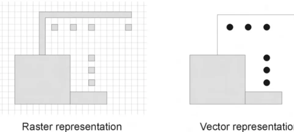
3.1 Geometric objects represented in Raster and Vector format . . . 17

3.2 Geometric objects can be represented in three different dimensions: 2d (a), 2.5d (b) [imgb] and 3d (c) . . . 18

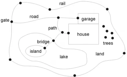
3.3 Example of a geographic map: a site with house and lake . . . 19

3.4 Examples of linestrings: simple linestring (a), simple closed linestring (b), non-simple linestring (c), non-simple closed linestring (d) . . . 20

3.5 Examples of Spline Curve and Bezier . . . 21

3.6 Polygons: simple convex polygon (a), simple concave polygon (b), simple polygon with hole (c), complex (non-simple) polygon (d) . . . 21

3.7 Geometry Collection Examples: MultiPoint (a), MultiLine (b), Mul-tiPolygon (c) and GeometryCollection (d) . . . 22

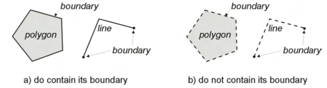
3.8 Geometric objects do or do not contain their boundaries . . . 23

3.9 Example of a Triangle Irregular Network . . . 23

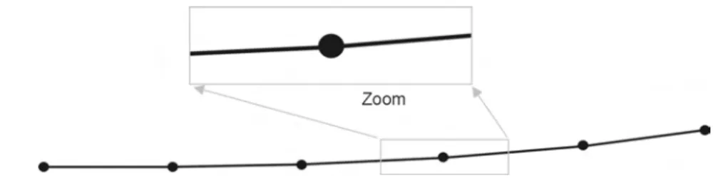
3.10 The polyline seems locally straight, but not straight at all . . . 29

3.11 Exact geometric computation in map overlay [BH98] . . . 30

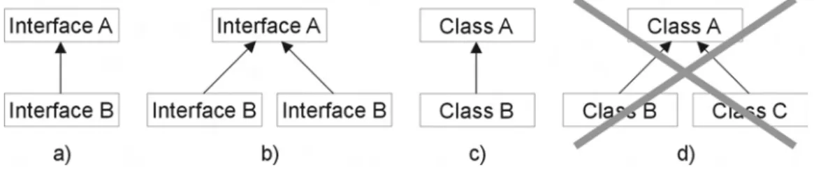
4.1 Inheritance in Java: Java supports multiple interface inheritance, but not multiple class inheritance . . . 34

4.2 Geometry in the conceptual model . . . 36

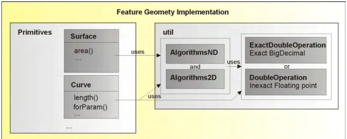
4.3 Metric operations are based on elementary operations, which use optionally floating point arithmetic or exact integer arithmetic . . . . 39

5.1 Object Hierarchy of the Feature Geometry . . . 42

(10)

6.1 The Doubly-Connected Edge List . . . 52 6.2 Vector and point translation to the origin of the coordinate system

for the orientation test of a point and a line segment . . . 54 6.3 Ring orientation test: if the the highest point, its predecessor and

its successor are ccw oriented, the whole ring is ccw oriented (a); in case of collinearity the x value order of its predecessor abd successor decides (b) . . . 55 6.4 The Point-In-Ring Test counts the intersections of the ring segments

with the straight line from the point into a direction: p1 and p4 lie outside the ring and have an even number of intersections. p2 and p3 lie within the ring and have an odd number of intersections. . . . 57 6.5 Example of a Map Overlay: Three thematic maps with country, city

and river information are overlaid into one map [imga] . . . 59 6.6 Set Operations between two surfaces . . . 60 6.7 Different types of Noding: The union of two curves (1) can be

noded partially in topologically equivalent representations (2) or completely (3) . . . 61 6.8 Theoretically, set operations like difference can produce non-closed

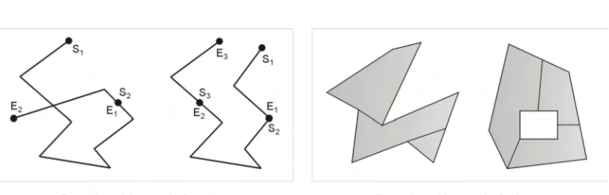
sets . . . 61 6.9 Merging ambiguousness: The lines in (a) and (b) are topologically

equivalent, but are defined by a different sequence of control points. The union of the curves in (c) is shown in (d). The object type of its final representation is ambiguous. . . 62 6.10 The difference between two CompositeSurfaces can result in objects,

which are not representable in conformance to the Abstract Specifi-cation . . . 63 6.11 The sweep line moves down to the next event point: As the event

point is an intersection point, the involved segmentsskandslmust

be tested against their new neighbours . . . 66 6.12 A noded graph with directed edges . . . 67 6.13 Finding all intersections in the overlay operation using the plane

sweep algorithm . . . 69 6.14 Internal graph representation . . . 70 6.15 The 4-Intersection matrix: its different configurations describe eight

topological relations between two regions (From [ECF94]) . . . 72 6.16 Interior, Boundary and Exterior of two Polygons: Polygon A

(11)

6.17 The 9-Intersection matrix: regions with holes can be separated ex-actly into the eight specified topological relations by additional dis-tinction of the polygon exterior (from [EH91]). . . 75 6.18 Disjoint geometric objects . . . 77 6.19 Examples of Touches relationships: Surface/Surface(a),

Surface/-Line (b), Surface/Point (c), Curve/Curve(d), Curve/Point(e) . . . 79 6.20 Examples of the Within / Contains relationship: Surface/Surface

(a), Surface/Curve (b), Surface/Point (c), Curve/Curve(d) and Curve/Point (e) . . . 80 6.21 Examples of the overlaps relationship . . . 80 6.22 Examples of the crosses relationship . . . 81 6.23 Examples of buffers: a positive buffer can be performed on a curve

(c2) and surface (s2), a negative buffer only on a surface (s3) . . . 83 6.24 Examples of centroids of geometric objects: a point set (a), a straight

line (b), a curve (c), a simple polygon (d) and a simple polygon with a hole (e) . . . 84 6.25 Centroid of a triangle (a) and centroid of a surface computed by the

centroids of the surface triangulation . . . 85 6.26 Triangulation by choosing a fixed point instead of partitioning the

surface . . . 86 6.27 Triangulation of a hole within a surface . . . 86 6.28 Examples of convex hulls: Surface (a), MultiSurface (b), MultiPoint

(c), straight Curve (d), Curve(e) and MultiCurve(f) . . . 88 6.29 The Graham’s scan algorithm computes the upper and lower hull

separately from left to right and deletes points which do not result in a right turn . . . 89

7.1 Hierarchy of TestSuites and TestCases . . . 93

B.1 Examples of Monotones Chains (from [viv03b]) . . . 103

(12)

1 Introduction

1.1 Context and Scope

With more than 80% of worldwide digital data making some reference to loca-tion or time [BLM00], the significance ofGeographic Information Systems (GIS)has rapidly increased in the last two decades. GIS are software systems which store, analyze, visualize and manage spatial data (a.k.a. geodata or geospatial data). Examples of such data range from traditional digital map data to survey data, satellite imagery, aerial imagery, GPS, sensor webs cell phone locations or any tabular database which uses location contents such as addresses, phone numbers, IP addresses, landmark names, and place names [OGC03]. The process of any type of digital computing using geographic data is calledgeoprocessing. Geocomputing is the umbrella term for both, geoprocessing and geodata.

In the past few decades, several geocomputing systems have been developed to store, visualize and analyse geodata, commercial GIS as well as free and open source GIS. The benefits of sharing geodata are manifold. However their reuse is often a cumbersome and error-prone task because of poor documentation, obscure semantics, diversity of data sets, and the heterogeneity of existing sys-tems in terms of data modelling concepts, data encoding techniques and storage structures [SL03].

(13)

Information systems’ ability to freely exchange all kinds of spatial informa-tion about the Earth and about objects and phenomena on, above, and below the Earth’s surface, and to run (cooperatively, over networks) software which manipulate such information, is calledGeographic Interoperability[OGC02]. Inter-operability has become an important issue to GIS vendors, providers and users. Generally, interoperability is achieved by standards. In research areas such as automobiles, televisions and radio, or the internet there are worldwide standards driven by industry. The gap in industry standardization of geographic informa-tion makes interoperability impossible.

As a result of the problem of non-interoperability, the Open Geospatial Con-sortium (OGC) was founded in 1994. It initialized the OpenGIS projectwith the goal of achieving a national and global infrastructure which allows geospatial data and geoprocessing to move freely and fully integrated with modern dis-tributed computing technologies accessible to everyone. Today, OGC has more than 330 government, academic, and private sector organization members [OGC], and it works together with theInternational Organization for Standardization (ISO) [wwwe]. The OGC is by far the most important standardization organization on geographic data and information systems.

(14)

Figure 1.1:Overview of the OGC Abstract Specifications (from [OGC05])

The Simple Feature Implementation Specification (SFS) [SFS05a] is an Implemen-tation Specification for the Feature Geometry Abstract Specification (FGAS) (topic 1) [OGC97]. It focuses on Distributed Computing Platforms (DCP) and specifies a simplified data model based on points, lines and polygons in two Euclidean dimensions. The SFS turned into a widely accepted geometry definition and was absolutely sufficient as a geometry implementation in many two dimensional open GIS. However, there are many applications where the representation and analysis of three dimensional data is needed, such as the calculation of drainage areas or flood and weather prediction. The only serviceable GIS solutions are commercial ones (such as ArcGIS). Three dimensional free or open source GIS are rare (for instance, GRASS or SAGA) and are either not based on open standards or functionally limited. The FGAS specifies a high variety of geometric objects to rep-resent real world entities more realistically, in up to three Euclidean dimensions. As the FGAS is an international ISO standard and provides codeable interfaces, it has a great potential to turn into an important data model definition for three dimensional geographic information.

(15)

further implementations. Up to date, no open source implementations of the FGAS GeoAPI interfaces, or of the FGAS in general have been completed or usable. The implementation of an international standard as free open source software, instead of commercial software, has many advantages. Open source software brings ben-efits to everybody involved:

• to the user: many governmental, academic and institutional organizations do not have the financial capabilities to invest in expensive software licenses.

• to the success of the project: open source software is transparent for users and developers. The risk of parallel efforts is minimized and there is a poten-tial contribution from and collaboration with other developers with the same intentions. Furthermore, an open source project may have good chances to be continued by other developers afterwards.

• to the developer: open source projects are likely to be spread and used worldwide, because they are free. If such a project provides an established solution, the developer’s reputation will benefit significantly.

GeoTools[wwwc] is a large open source GIS library; it works in close collabora-tion with the GeoAPI project and implements their interfaces wherever possible. GeoTools is used in many open source applications and has a vital community of developers. As there is a high potential for projects to benefit from the efforts and contributions of other developers and groups, the hosting of a new implemen-tation of the FGAS as a subproject in the namespace of GeoTools brings optimal conditions for the project’s success.

1.2 Objectives of this work

(16)

project.

The complex data model specified by the FGAS cannot be fully implemented within the scope of a graduation thesis. Therefore, the objective of this work is to provide an implementation of the FGAS, which can substitute an implementation of the SFS (as the SFS defines a simplified subset of the FGAS). At the same time, the proposed implementation should not be constraint to further development. Spatial analysis algorithms of three dimensional (3d) data are unproportionally more complex than the ones for two dimensional data (2d). The implementation of this thesis should be able to store 3d data in all implemented data types, but only support 2d spatial analysis. However, the design of the implementation’s architecture should allow algorithms which support 3d data to be later extended.

This work follows earlier implementations [RJ05] covering mainly the root object as well as the primitive and the coordinate package. In the current work, these packages were reviewed, extended and tested. Furthermore, missing spatial operators were designed, implemented and tested, including the analysis of oper-ators envolving complexes and primitives.

An important issue in this work is the reuse of existing code and the consid-eration of former research results on this area. That is, a research, as complete as possible, of the existing work in open source FGAS and SFS implementations to benefit from that work and create a high quality open source implementation. One of the most used foreign source codes in this thesis is the one of the JTS (see Chapter 2.3.2). At some parts of the implementation of spatial analysis operators, JTS source code was copied and modified under LGPL terms.

The objectives of this implementation can be summarized as follows:

• Implementation of basic FGAS data types, particularly of the primitive and coordinates package. The implementation should be able to store and anal-yse 2d geographic data in an extension functionally comparable to the SFS.

(17)

• The implementation should be extendable and support the implementation of three dimensional analysis operations. Therefore, it shouldprovide the differentiation of dimensionalityof geographic data.

• Analysis of thepossibilities of numeric precisionand selection of the most appropriate precision for the implementation.

• Robustness is an often faced problem in numerical algorithms. All algo-rithms should be implemented in a robust manner.

• Many geometry implementations result in memory problems when loading large data sets. The implementation should consider a solution to realize

persistencefor a future implementation.

A geometry implementation is a technologically complex task. As a result of the limited time for a thesis, this research does not include all issues regarding such an implementation:

• This research focuses on the geometry of the FGAS. The topology data types defined by the FGAS are not considered.

• The focus of the data types is on primitives and coordinates. Complexes and aggregates are not aimed at being implemented.

• The FGAS defines a manifold ofGM_CurveSegments. This implementation will exclusively implement theGM_CurveSegmenttypeGM_LineString. The remainders, such as Splines, Arcs and Beziers will not be implemented.

• This implementation does not consider the implementation of a Coordinate Reference System.

1.3 Thesis Structure

The remainder of this thesis is organized as follows.

(18)

Chapter 3 introduces geometric fundamentals. It starts with raster and vec-tor models and the dimensionality of geographic data. It also demonstrates the possibilities of geometric modelling in order to represent geographic information. Finally, the large research area of computational geometry will be shortly intro-duced and implementation relevant aspects such as robustness and performance will be analysed.

Chapter 4 discusses the general implementation aspects and design decisions in this work’s implementation. The topics are separated into programming lan-guage, implementation interoperability, the design of a dimension and precision model, and data storage and persistence.

Chapter 5describes the data model defined by the Feature Geometry Abstract Specification, its hierarchy and its dependencies. The geometry root object, prim-itives, aggregates, complexes and the coordinate support types are discussed, particularly in terms of the implementation.

Chapter 6 discusses structural and algorithmic issues necessary to realize the spatial analysis operators. The chapter discusses an appropriate data structure for a topological graph, geometric predicates and basic algorithms, set theoretic operations, relational Boolean operators, and constructive and metric operations. Specially in the discussion of set operations and relational Boolean operators, it explains design decisions and demonstrates possible weak points of the FGAS.

Chapter 7comments on the testing methodology used to verify the implemen-tation of the data types and spatial analysis operations.

(19)

2 Interoperability

2.1 Background

Interoperability has been a basic requirement for modern information systems for the past two decades [On]. It brings together heterogeneous and distributed infor-mation systems [SL03]. Although work is becoming constantly more specialized, there is a rising need to reuse and analyse data in different work areas. As a result of great progress in interconnection through the Internet, data and information sharing has gained increasing attention. Progress achieved in computing and com-munication technology constantly surpasses technology’s capabilities; hardware becomes faster and smaller, memory gains more capacity, network performance rises and the diversity of input and output devices seems unlimited. Such tech-nologic advances have changed the GIS trend from mainframe GIS to desktop GIS, from desktop to client/server GIS, and from client/server to omnipresent Distributed GIS (DGIS). The trend to DGIS was only logical as hardware, software, operation system, user and data are inherently dispersed in the environment.

Distributed Computing offers the potential to improve availability, reliability, performance, scalability and data sharing. From the point of view of software engineering, interoperability in DGIS yielded two research topics [Chu01]:

• Geodata sharing: this involves research on metadata standards, semantics, autogeneration, management and simplification in order to make geodata usable and understandable for all users.

• GIS service accessing: this topic is engaged in the question ’how a client can access services and geodata from the web’. Currently there are two pos-sibilities to transfer Geodata from the server to the client: images or vec-tor data. The W3C and OpenGIS recommendations and standards on dis-tributed architectures gain much research attention.

(20)

availabil-ity through replication, performance through parallelism and flexibilavailabil-ity and scalability through modularity, which are typical of distributed computing. Furthermore, distributed systems can be dynamically configured during the running time.

Approaches to GIS interoperability can be divided into three categories [Chu01]:

• Open Geodataimproves the interoperability between geographic data. This is accomplished with the use of standardized data formats such as XML or GML.

• Open Geoprocessing is any kind of digital computing using geographic data, e.g. service models or application logic models.

• Open Geocomputingis the umbrella term for Open Geodata and Open Geo-processing to support a neutral, geocomputing environment.

2.2 Interoperability Levels

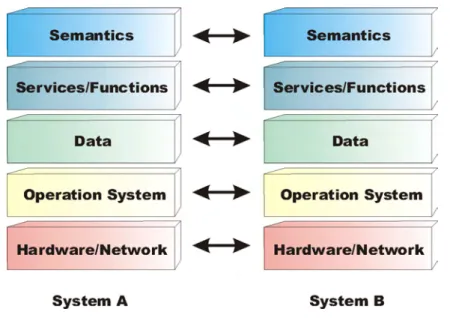
Interoperability can be achieved at certain levels. Goodchild et al. [On] defines a model which distinguishes between three generations of system interoperability: System, data and information/knowledge. However, particularly for interoper-ability between two or more geographically distributed GIS, such a model is able to distinguish levels in more detail. Figure 2.1 shows a distinction into five levels [Chu01].

Hardware and networkis on the lowest level. The interoperability at this level is given by network interface cards within computers, cables connecting the cards and network protocols, which provide a standardized communication language to encode and decode the data. Examples of this type of interoperability are TELNET or ISO standardizations such as TCP/IP (Transmission Control Protocol/Internet Protocol), which secure interoperable communication over the Internet. The hard-ware and network level refers to the data link and network layer of the ISO/OSI reference model.

(21)

Figure 2.1:Interoperability Level

system. This level refers to the application layer of the ISO/OSI reference model.

Data interoperability is on the middle level. It involves the interoperability of spatial data, which can be downloaded or interchanged based on a metadata standard (for instance, the TC211 metadata standard). If interoperability is on this level, the system identifies the data format and translates it to the user’s. Data access through database queries such as SQL is also referred to as data interoper-ability. Given that data model and data semantics are unknown; the main problem in this level is the need for prior knowledge about which data is available and how to extract real information from them.

The fourth level describes interoperability at the stage ofservices and functions, i.e. the interoperability between components, modules and methods. OGC’s specifications are efforts to realize this level of interoperability and to provide a global data model with knowledge about available spatial analysis functions and GIS services. In the context of the FGAS, methods are provided to access data’s properties and analysis of and between data objects. Although users can access all properties and analysis results through functions, knowledge of the data semantics is still required.

(22)

the semantics of data, i.e. complete interoperability in data, information, rules and knowledge. This kind of interoperability is hard to achieve as most of the data models conceptualize properties of the world in different manners. There are still no established approaches at this level of interoperability.

The lower two levels are typical IT (Information Technology) issues, whereas the upper three levels are typically assigned to GIS research. Therefore, these three levels are also refered to as GIS interoperability.

2.3 Interoperability Approaches

Distributed GIS and the sharing of geographic data are up-to-date issues as the market’s demand shows. For example, there are worldwide government pro-grams to establish infrastructures for geographic information on a high level as well as on a low level. The project INSPIRE (Infrastructure for Spatial Informa-tion in Europe) is a program of the European Union (EU) to establish a unified infrastructure for European geographic data. In Germany several States maintain similar projects, often in cooperation with one another (for instance, GDI-NI1_and GDI-NRW2). Almost all of those programs are based on seminal standards for GIS interoperability, such as those published by the OGC.

GIS interoperability can be characterized as follows:

• Openness and Transparency: GIS software designers and developers should provide open models and systems.

• Extensibility and Exchangeability: GIS service providers should design data and functionality in a way that is easy to exchange among GIS.

• Simplicity and Similarity: GIS users should be able to easily migrate from one GIS application to another. The graphical user interface (GUI) of an application should be usable with common knowledge and experience.

All efforts which aim at GIS interoperability should strongly consider these aspects in order to become a worldwide-spread and accepted interoperability norm. The most important approaches in GIS interoperability which follow these aspects are listed below.

1_{Geodatenportal Niedersachsen}

(23)

2.3.1 ISO/TC211

The International Organization for Standardization (ISO) [wwwd] is the world’s largest developer of international standards. The preparation of international standards is normally realized by ISO technical committees, divided into sev-eral subjects. TheISO/TC211 Geographic information/Geomatics[wwwe] is the ISO technical committee dedicated to the standardization of digital geographic infor-mation, i.e. information concerning objects or phenomena that are directly or indirectly associated with a location relative to the Earth.

In 1998, ISO/TC211 and OGC signed an agreement so that both organizations could take full advantage of mutual contributions. One part of their collaboration is the inclusion of ISO/TC211 documents into the Abstract Specifications of OGC. In turn, OGC can submit Implementation Specifications as proposals for interna-tional standards ([OGC05], page 3).

2.3.2 Open Geospatial Consortium

The Open Geospatial Consortium (OGC) is an international non-profit trade industry organization, which is currently composed of more than 330 companies, government agencies and universities. OGC supports interoperable solutions to "geo-enable"the Internet, wireless and location-based services, and mainstream IT.

Vision and Goals. The vision of OGC is the full benefit of society, economy and science through the integration of digital spatial resources into commercial and institutional processes worldwide. OGC’s strategic goals are to [OGC]:

• Provide free and openly available standards to the market.

• Be the worldwide leader in the creation and establishment of standards that allow geospatial information and services to be seamlessly integrated into business, civic, web and enterprise applications.

• Facilitate the adoption of open, spatially enabled reference architectures in enterprise environments.

(24)

• Accelerate market assimilation of interoperability research through collabo-ration.

Specifications. The OGC uses specifications to achieve geospatial interoperabil-ity. Those specifications define [Chu01]:

• Open Geodata Model, which is a general set of geographic data types to model geodata.

• OpenGIS Web Services, firstly, to access and process geographic types defined in the open geodata model, and secondly, to support the sharing of geodata within communities which use a common set of feature definitions and the translating of geodata between communities which use different sets of feature definitions.

• Information Community Model to help communities maintain their defini-tions and catalogue data sets they share, and to provide an efficient and accurate way to help communities with different feature definitions share geodata.

OGC certificates implementations if they are in compliance with an OGC stan-dard. Implementations of the OpenGIS Specifications can be categorized into Compliant Productsand Implementing Products. Compliant products are software products which comply with OGC’s OpenGIS Specifications. These products have been tested and verified through the OGC Testing Program and will be registered as a compliant on the OGC site. Implementing Products are software products which implement OGC’s OpenGIS Specifications, but have not been verified yet. Most of the products are implementing products, since there are not compliance tests available for all OGC specifications.

(25)

aspects. Therefore, independently developed implementations of an Implementa-tion SpecificaImplementa-tion should be absolutely interoperable.

Feature Geometry Abstract Specification. The geometry layer is located at the lowest level of a GIS. It translates geographic entities, which represent Fea-tures (i.e. real world objects), into geometric entities and allows special analysis functions on and between them. TheFeature Geometry Abstract Specification (FGAS) [OGC97] is the OGC document which defines the reference model of this layer. It separates geometric objects into primitives, aggregates and complexes in up to three Euclidean dimensions. In contrast to traditional GIS geometries, it provides a great diversity of objects to describe geographic data (such as the use of curvilin-ear curve segments) and hence has the potential to describe the form and position of real world objects as realistic as possible. The ISO approved the FGAS as an international standard (ISO19107). As a result, the standard has gained more and more research interest [PvOV00][Kuh05]. Throughout this thesis, the FGAS is also referred to as theAbstract Specification.

The FGAS implementation approaches researched in this work are still not fin-ished. TheGeoOxygeneproject [cog06] aimed at providing a complete DGIS. The project is on hold, because too many members moved into other projects. The deegreeproject provides a set of OGC compliant web services and implements a set of classes specified by the FGAS. However, its implementation is based on the JTS, a 2d geometry implementation which is explained below. Hence, the degree project is not 3d data type compatible. The GeoTools project (also explained below) started a similar project, wrapping JTS classes into the data model of the FGAS.

Simple Geometry Implementation Specification. The Simple Geometry Implementation Specification (SFS) is an Implementation Specification based on the FGAS. It focuses on Distributed Computing Platforms (DCP) and is based on a simplified 2d data model which represents geographic data in points, linestrings and surfaces. It defines a general architecture [SFS05a] and three implementation specifications for the DCPs SQL [SFS05b], CORBA and OLE/COM.

(26)

com-pliant to the SFS. It is a robust and running time efficient implementation and is used worldwide in several open source projects such as JUMP, UDig and GeoTools. However, JTS does not support any type of persistence, consequently it sometimes faces memory problems when loading large data sets. Another implementation of the SFS was done in the master thesis of Fei [Chu01]. Other implementations may be available, however the JTS is the most used one.

2.3.3 GeoAPI and GeoTools

Abstract Specifications do not provide so clear semantic definitions of the data types’ functions and attributes as Implementation Specifications do. A clear def-inition of the semantics is necessary in order to provide interoperability between implementations of Abstract Specifications. The GeoAPI project [wwwb] is ded-icated to this task, specifying and publishing interface class-files which shall be the basis for further interoperable implementations by the GIS community. These interfaces, published by the GeoAPI project, have been generated directly from the TC211 documentation. Attributes of geometric objects and some of the anal-ysis operators can be accessed bygetter andsetter methods to conform with the conventions of JavaBeans.

(27)

3 Geometric Fundamentals

One of the most basic aspects inGeographic Information Scienceis how to represent geographic information. Datasets showing a small portion of the Earth are usu-ally projected to the classical Cartesian Coordinate System, the Euclidean spaces. Since a flat projection cannot show the whole world in an uniform scale, there are several kinds of projections [Goo00]: azimuthal projectionusing a plane tangent to the Earth in the centre of the area which shall be mapped, conical projection (like Alber’sandLambert’s projection) and cylindrical projection using a cylinder tangent to the Earth. In theMercator projection this cylinder is tangent along the Equator, in theTransverse Mercator projectionit is tangent along a line of longitude.

Another discussion is about the definition of a global reference system. There are many approaches like the division of the Earth in several subdivisions which are mapped separately. However, the following part of this thesis will assume that geographic data is always mapped into the Euclidean plane.

3.1 Spatial Data Representation types

Since the beginning of raster and vector models, there has been discussion about which modes better represents spatial data. It is the choice between an entity based view, where space consists of single objects with its geometry and attributes, and a space based view, where each point in space has properties [FPM]. Both approaches have their advantages and disadvantages.

(28)

Figure 3.1:Geometric objects represented in Raster and Vector format

on a raster model: small units allow higher precision, but need more memory. Bigger units save memory but neglect precision. In spatial analysis, raster models offer advantage in operations such as the intersection of two geometric objects. In contrast, access methods to locate certain objects are difficult to realize.

Avector modelis entity oriented. The entities are represented by their geometry and attributes. Early versions sometimes saved collections of geometries without internal structure and relations. Those models are derogatively called spaghetti models. Actual vector models are well structured and may even explicitly store topological relationships among entities. Vector models achieve a good level of accuracy. Objects can be located efficiently, for example in spatial databases using the entities as search keys. On the other hand, operations like the buffer computa-tion are less efficient in pure vector models.

Today’s commercial GIS often offer hybrid systems which combine both the raster and vector model and support the necessary conversion between them. Since the Feature Geometry Abstract Specification defines the vector model within theOpenGISapproach, the rest of this thesis will be focused on the vector model.

3.2 Dimensionality

(29)

valuesxandy). Thethree dimensional Euclidean spaceadds information of height by a third coordinate valuez. Three dimensional data is distinguished intwo point five dimensional (2.5d)data and realthree dimensional (3d) data. It is important not to confuse theEuclidean dimensionwith thetopological dimension, also known as the Lebesgue covering dimension. The topological dimension of a point is zero, of a line is one, of a region is two and of a solid is three.

Figure 3.2:Geometric objects can be represented in three different dimensions: 2d (a), 2.5d (b) [imgb] and 3d (c)

Figure 3.2 shows examples for the different models. Two dimensional data is located on the surface of the Earth (see illustration (a)). A 2d data model is sufficient to represent most of today’s geographic data since it does not depend on height information. Typical examples are street or vegetation maps. A dig-ital representation by 2.5d data (see illustration (b)) is also called Digital Terrain Model (DTM)or Digital Elevation Model (DEM). These data models are used in all areas where the height information is necessary, for example for the calculation of drainage areas or flood or weather prediction. A three dimensional data model represents the real world’s objects best as it can model objects on top of each other like a riverbed, the height of the water surface and a bridge above (see illustration

(30)

Traditional vector based GIS usually use a two dimensional data model, based on the vast difference of complexity between analysis algorithms for 2d and 3d data. For many problems there are still no efficient algorithms which work in three dimensions. Many systems offer terrain models in order to visualize surfaces bet-ter. Real 3d GIS are still very rare. Particularly there are almost no useful Open Source products. However, there is a high need of representation and analysis of data in 3d and hence its representing data structures and algorithms will be a hot field of research in the next years. The Feature Geometry Abstract Specification supports objects up to three dimensions and is accordingly able to fulfil the actual needs of the GIS community. Since it is the only ISO standard for a 3d geometry model, it will gain more attention and importance in future.

The trend of GIS could lead to the fourth dimension which represents the time. Objects can modify their spatial properties and their attributes by time. This mod-ification can be saved in fourth dimension values. The majority of actual GIS do not treat the time aspect but may in future since it is an important point which gains more and more attention due to rising application possibilities.

3.3 Geometric Modelling

3.3.1 Spatial Entities and relationships

Figure 3.3:Example of a geographic map: a site with house and lake

(31)

geometric entities are more complex, like solids. Figure 3.3 shows a geographic map represented by geometric objects.

Figure 3.4:Examples of linestrings: simple linestring (a), simple closed linestring (b), non-simple linestring (c), non-non-simple closed linestring (d)

(32)

the analysis of and the operation on continuous curves are disproportionately more complex and complicated, most of the data structures assume that lines are composed of straight line segments.

Figure 3.5:Examples of Spline Curve and Bezier

Figure 3.6:Polygons: simple convex polygon (a), simple concave polygon (b), simple poly-gon with hole (c), complex (non-simple) polypoly-gon (d)

(33)

but implicate a raise of complexity and complication of its analysis.

Figure 3.7:Geometry Collection Examples: MultiPoint (a), MultiLine (b), MultiPolygon (c) and GeometryCollection (d)

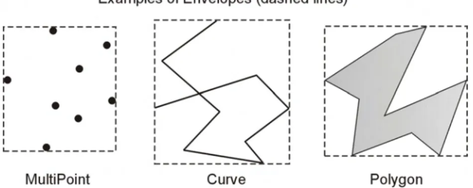
Some geographic objects may be separated, i.e. not physically connected, or by other reason not be representable as a single point, line or region. In order to represent such geographic entities as a single geometric objects,geometry collections were introduced (see figure 3.7). In general, they are an unordered set of geometric objects. A MultiPoint contains only points (see example(a)), a MultiLine contains only lines (see example (b)) and a MultiPolygon is composed only of polygons (see example(c)). A geometry collection can hold points, lines and polygons (see example(d)). In some definitions the entities within a collection may intersect, in others they have to be disjoint. Their names may differ in other publications. For example, the FGAS specifies them within theAggregatefamily asMultiPrimitives: MultiPoint, MultiCurve andMultiSurface. Geometry collections are often used to describe a set of single instances as trees, streets, countries or even a whole site as in the example in figure 3.3 above.

(34)

Figure 3.8:Geometric objects do or do not contain their boundaries

do not. This depends on the definition of the data model. Figure 3.8 illustrates examples of a polygon and a line which do contain their boundary (see example (a)) and a polygon and a line which do not contain their boundary (see example (b)). The latter are drawn with dashed boundary lines.

Another property of geometric objects is theirorientation. In general, the orien-tation of a line reflects its direction. A line which is negative oriented is called the twin(ormate) of a positive oriented line with the same control points. The orien-tation of regions generally refers to the direction in which the region’s upper side points.

3.3.2 Cell Complexes

ASubdivisionis the resulting graph from a subdivision of edges of a GraphG, i.e. a selection of edges of G. A subdivision of a topological space can be seen as a subset of the entities or its components within this topological space. In algebraic topology, there is a well-established theory which represents subdivisions of the topological space ascells.

(35)

Simplicial complexes are a special type of cells. They are composed of points, lines and triangles. Simplicial complexes have been used by GIS to represent simply-connected polygons, such as TINs (Triangle Irregular Network). Figure 3.9 illustrates a TIN. This technique is elegant, however, it is very space consuming because of the possibility of a large number of triangles represented by edges and points. A similar approach uses convex cells to represent features. Suchregular cell complexes correspond to planar subdivisions (such as simple polygons) and are commonly used in CG. Cell complexes are suitable to model maps that do not contain points or lineal features.

The most general cell structure in algebraic topology is theCW-complex[AL69]. In a two dimensional space a CW-complex is a subdivision which does not contain its limiting boundary. CW-complexes are capable of representing features such as the ones with cuts incidents in the boundary. However, CW-complexes only rep-resent simple regions, therefore they cannot reprep-resent certain features essential to GIS, such asislands1. Some efforts have been undertaken to adapt CW-complexes to GIS data, but no substantial progress in data structures or computational tech-niques has been made so far [FPM].

3.3.3 Topological Data Structures

Topology is the structure of space. Relationships between subdivisions such as proximity relationship, intersections or equality are calledtopological relationships. [Rös98] thoroughly discusses such topological relationships in GIS. Section 6.4 illustrates examples which involve this implementation.

Data structures, representing the geometry of an object as well as its topological relationships in a subdivision, are calledtopological data structures. These structures can help turn computational geometry problems, for instance the point-in-polygon containment, into combinatorial problems. Because those structures already store such topological relationships; they need only be evaluated. Therefore, a well chosen topological structure can bring tremendous performance benefits to spatial operations.

Examples of topological structures are the Doubly-Connected Edge List (DCEL) (which is discussed in section 6.1) by Preparata [PS85] and thehalf-edge structureby

1_{A divided region, i.e. two disconnected regions which represent a single feature, is also referred}

(36)

Mäntylä [Män87]. In addition, there are structures which have been specially cre-ated for certain representations such as triangulation. For instance, a topological structure for a triangulated surface may store each triangle together with its three neighboured triangles to provide fast access to all components in spatial opera-tions. Moreover, the FGAS also defines a topological structure in close accordance with its data model.

3.4 Computational Geometry

3.4.1 Application domains

Computational geometry (CG) is the study of algorithms to solve problems rep-resented in terms of geometry. The rapid advances in computer hardware and visualization systems over the past few decades has multiplied the possibilities of CG in geometric computing. Thus, CG plays a key role in almost every area of science and engineering, from design and manufacturing to molecular biology (see [For96]). In the following, a small overview of the most common application domains [dBvKOS97] is given.

Computer Graphics. Computer graphicsdeal with the creation images of mod-elled scenes for display on a screen or other output device. The scenes can vary from two dimensional maps to three dimensional realistic constellations which include light sources, textures etc. Since the objects in the scene are geometric objects, CG plays a big role in computer graphics and allows algorithms to com-pute images such as computing light diffusion, shadows, views from different angles and so on.

Robotics. Roboticsis the study of the design and use of robots. Robots act in three dimensional space. Both the robots and their environment are geometric objects. CG supports the field of robotics by offering algorithms that optimize the robots’ behaviour (e.g. find optimal paths, movements or order of actions) and attributes (e.g. position of fixed robots).

(37)

simulations. Once a product is designed,computer aided manufacturing (CAM)can help to manufacture the product. This involves many geometric problems.

Geographic Information Systems. Geographic information systems store geo-graphical data like shapes of countries, streets, rivers or buildings, height of moun-tains, type of vegetation or population density. All these entities are internally rep-resented by geometric objects like points, lines and polygons. CG is the medium that gives a GIS the power to analyse the stored data for the purpose of deriving new information, extracting results or understanding its nature and significance. For example, CG algorithms can find all countries that contain a certain river, cal-culate the drainage area in case of big rain storms, simulate flooding in order to help in decisions how to prevent them, simulate wind and cloud development in order to provide a weather prediction and much more.

Other application domains. CG has become a central component in many more areas. Examples are molecular biology, where molecules are represented by collections of intersecting balls (atoms) and CG algorithms could perform the surface computation of a molecular, or pattern recognition like letter recoginition in scanning programs.

CG can be divided into two types:Combinatorial computational geometryand

numerical computational geometry. The latter one is typically used in geometric modelling like CAD/CAM. The former one is generally known as computational geometry or algorithmic geometry and includes all kinds of algorithms that deal with geometric entities. Many examples of the numerical CG can be found in the GIS area, where Boolean operations on polygons, closest pair of points, convex hull, Delaunay triangulation, line segment intersection, minimal convex decom-position, polygon triangulation and point in polygon tests are typical algorithms. [FPM] introduces into the wide field of CG application in GIS.

Since the implementation of CG algorithms is a focus in the implementation of this work, most of the used algorithms are explained in detail in the course of this thesis.

3.4.2 Robustness and Performance

(38)

sufficiently. Accuracy is an issue of how to collect high quality data. In GIS, one can consider horizontal and vertical accuracy to measure the accuracy of a geo-graphic position. In contrast, precision is the level of exactness of the information digitally represented in a digital database or data type (for example a concrete floating-point or integer arithmetic implementation). Hence, data may be very precise, but still inaccurate. As the development of GIS components such as a geometry is not directly engaged in the collection of data, the sequel of this section will be focused on precision issues.

There are several possibilities of precision, i.e. how and where to store infor-mation. In GIS, such types of precision are sometimes calledprecision models. The most common precision models are:

• Fixed precision.The value will be rounded according to a scale factor: point.x = round( point.x * scale ) / scale

point.y = round( point.y * scale ) / scale

A scale greater than one means that the precision point is to the right of the decimal point, i.e. we have a high precision (more bits). A scale smaller than one means that the precision point is to the left of the decimal point, i.e. we have a smaller precision (less bits). Result values of computation will be rounded by the rules above and have the same number of digits as its input values. Raster models always accord to fixed precision, because they use a homogeneous unit scale.

• Floating point precision. The values will use the full precision provided by the according floating-point data types based on the IEEE floating-point standard (seeIEEE Floating-Point Standardin Appendix B). In Java, these are the elementary data types floatanddouble. Computation results may have more digits than the input values.

• Exact precision. Exact arithmetic is the general term for arithmetic which realize exact results for input data in computation without loss of precision by rounding. In general, this is achieved by integer and rational arithmetic. Exact geometric computation is discussed below (seeExact geometric compu-tation) in detail.

(39)

can set axioms of arithmetic out of order [Sch98]. For instance, the evaluation of the term

3·0.4 = 1.9999999999999999

(evaluated with JDK 1.5) is a typical floating-point rounding error. However, floating-point computation is hardware-supported (see IEEE Floating-point stan-dard, section B) and hence very fast. A comprehensive work about floating-point arithmetic and its weak points was given by Goldberg [Gol91].

Such rounding-errors are responsible for robustness problems. Inexact results can be used in combinatorial computations and make the complete algorithm fail. Schirra defines that ".. implementation of an algorithm is considered to be robust if it produces the correct result for some perturbation of the input. If the perturbation is small an implementation is called stable ..." [Sch98]. As such stability is referred to numerical computation it is also called numerical stability. Schirra and [LY01] review robustness and precision issues in a broad and detailed manner.

A wide spread approach on how to implement algorithms in a stable way is the use of athreshold value Epsilon (). This technique follows the rule of thumb "If something is close to zero it is zero". A trigger valueis added to a numerical value to test whether this value is (almost) equal to another numerical value. The original intention is that the difference between two numerical values can be that small that, in practice, both values can be assumed to be equal. A big problem is the choice of. In practice it is a tiny constant which value is found following the Try-and-Error process until all current tests work for the input data and no errors occur. The technique of finding anvalue is calledepsilon-tweaking[Sch98].

(40)

Figure 3.10:The polyline seems locally straight, but not straight at all

Consequently, the use of Epsilons can help in some situation, but may result in later robustness problems. Typical examples of robustness problems occur in the computation of the intersection point between two line segments, the Point-Line Orientation test and the Point-In-Ring test (seeGeometric Predicatesin section 6.2). Another problem, which occurs in practice is thedimensional collapse: Due to miss-ing precision or roundmiss-ing errors the topological dimension of an operation result is lower than the expected dimension. For instance, in the event that the precision is not high enough, the intersection between two very small regions may result in a single point or a line instead of a region (see [viv03b] for further explication).

The following part of this section addresses possibilities to avoid rounding errors without using Epsilons.

Exact geometric computation. The field of exact geometric computation has turned into one of the biggest issues in CG research. Exact geometric computation means the algorithms make correct decisions for all input data, not only for some perturbation of it. It is an approach to secure the robustness of algorithms.

There are many approaches for the realization of exact computation:

• Integer arithmetic.Integer arithmetic is based on binary representation and binary arithmetic operations. It can result in an overflow, but not in rounding errors. The use of arbitrary precision integers eliminates the overflow prob-lem. Since integral input is usually bounded in size (as the 16-bit elementary data typeint), some approaches use multiple precision integer with a fixed precision according to the binary size of the input data.

(41)

In general, divisions are typical reasons for rounding errors. Rational arith-metic avoids divisions, or better, they are postponed: a_b ÷_dc = a·d_b·c

• Homogeneous Coordinates.Homogeneous coordinates can be used to rep-resent the input data. Homogeneous coordinates use an additional ordinate, which can serve as a common denominator, and therefore avoid divisions.

• Symbolic and implicit representation. The result data is not directly com-puted, but only represented by its original input data. A numerical number as a result of complex computation can be represented by an expression tree which reflects the history of the computation of this numbers [MNU97]. An intersection point, for example, can be represented by the two line segments which intersect.

Figure 3.11 shows the map overlay process suggested by Brinkmann and Hin-richs [BH98]. As the algorithm uses the exact input data, result data must be rounded to the internal geometry precision afterwards.

Figure 3.11:Exact geometric computation in map overlay [BH98]

(42)

replaced a floating-point arithmetic package by a rational-arithmetic package in a Delaunay triangulation implementation. The results of the experiment showed that the implementation using rational arithmetic was about 10.000 times slower than the floating-point implementation. However, Güting presented an integer arithmetic based geometric domain calledREALM[GS93] [RHG], which underlies the spatial data types and seems to be more efficient.

Often not all operations must be implemented in a robust way and computed exactly. In fact, to construct complex robust algorithms or algorithms which offer the correct result for the majority of cases, only a few operations need to be imple-mented in a robust manner. This theory was adapted by the second approach. It considers certain geometric primitives which are implemented by a hidden technique to assure exact results. Thus, the exact computation is not implemented at every level of elementary arithmetic operations (Addition, Multiplication, etc.). The package of basic algorithms of Fortune and van Wyk follows this technique [FW96] and shows an immense run-time advantage in comparison to the first approach.

Adaptive Evaluation. As mentioned above, geometric algorithms based on floating-point arithmetic compute correct results most times and fail only in spe-cial cases. However, in practice, algorithms work correctly with floating-point arithmetic most of the time as well. Hence, the substitution of all floating-point computations by exact computations would result in a huge performance over-head which is unnecessary. Adaptive Evaluation tries to evaluate exact results only when needed. Stefan Schirra [Sch98] gives detailed explanation and a broad overview of implementations for this technique, which is also calledlazy evalua-tion.

(43)

In [BH98], Brinkmann and Hinrichs implement a floating-point filter and show how to combine imprecise floating-point arithmetic with exact integer arithmetic to achieve exact computation of determinant signs. Implementation experiments showed that the integer arithmetic implementation is about 50 times slower. Thus, the overhead of error-bound-computation is by far the better solution.

There are more approaches of exact computation like the interval arithmetic which is based on approximation and error bound, defining an interval that con-tains the exact result. [Sch98] reviews this idea as well.

As stated before, not all algorithms have to be implemented in a robust manner to achieve sufficient results for the practice. In most of the cases, approximated results, which may be rounded numeric floating-point values, are sufficient so that floating-point algorithms deliver correct results and only fail occasionally. [Sch98] states correctly that this is given by the fact that almost all input data in geometric algorithms arerealsgiven in floating-point or even integer arithmetic. The selec-tion of the algorithms, which shall be implemented robustly, depends on its later application. For example, it might not be noticeable when a single point of a con-vex hull is lightly slighted aside, but a test which determines whether a point lies on the left or right side of a line segment can result in extensive errors if it is not cal-culated correctly. Generally, the implementation of an algorithm in a robust way is recommended if the procedure creates decisive input data for another algorithm.

(44)

4 Implementation Aspects

A geometry data model is a complex data structure. The correct implementation of all semantic properties and relations of and between geometric objects requires a deep understanding of the data model. Though the data model is a core aspect in a geometry implementation, it is not the only one. Many GIS have shown weak points. This chapter discusses implementation relevant aspects which address the problems turned up in the development and use of previous GIS geometries (i.e. their data model) and explain how this implementation deals with them.

4.1 Programming language

One of the most basic and important choices is the one of the programming lan-guage. This should not only be the one which covers best the needs of the actual problem, but should also consider the language of the environment in which the geometry will work. A system with heterogeneous languages make object translations from one language to another necessary. In distributed systems, those aspects are not often a problem, but do still cost performance and, in practice, a geometry rarely will be installed separated from its above GIS layers.

By the nature of its problem, the object oriented (oo) technology is the most appropriate to implement the data model. The data model specifies data types which shall represent real world objects and follow a clear hierarchy with object inheritances. Object oriented features likemethod overloadingare ideal to define a general solution for higher objects (i.e. objects on top of the hierarchy), and more specialised solutions for certain types in a lower position within an inheritance hierarchy.

(45)

superclasses. This is not possible in Java (see illustration (d) in figure 4.1). How-ever, Java overcomes this limitation by allowing multiple interface inheritance, instead of multiple class inheritance (see illustration (b) in figure 4.1).

Figure 4.1:Inheritance in Java: Java supports multiple interface inheritance, but not mul-tiple class inheritance

The implementation in this work was done in Java due to its advantages spe-cially in portability. C++ is a high-performance language, but its code depends on the operation system on which it runs. Java source code is platform independent and will be compiled and translated into machine specific code by theJava Virtual Machine (JVM). Platform independency is one of the main requirements on OGC technologies [OGC03]. Furthermore, Java has one of the largest internet commu-nities. Many GIS, which often contain components based on OGC specifications, were implemented in this seminal oo language. The free open source toolEclipse was used to organize and develop the implementation of this work. It is a power-ful and widespread Java IDE (Integrated development environment) which offers a comprehensive list of functions to support the developer.

Coding Conventions. Open source software is usually not programmed by a single person, but rather by a community of programmers from different places, often even from different countries. This implementation works as a basis for future work by the GIS community (for example GeoTools). Coding conventions have become a de facto standard. They are important for a number of reasons (from [Sun06]):

• 80% of the lifetime cost of a piece of software goes to maintenance.

• Hardly any software is maintained for its whole life by the original author.

(46)

• If one ships a source code as a product, one needs to make sure it is as well packaged and clean as any other product created.

The source code of this implementation conforms to the SUN coding conven-tions [Sun06] in order to make it uniform and understandable. The following naming conventions were defined by SUN:

Type Rules Examples

Packages Package names have to be written in lower com.sun.eng

case ASCII letters and should be one of the org.geotools.geometry.iso top level domain names, followed by names

according to the organization’s internal own naming convention

Classes Class names should be nouns with the first class Curve;

& letter of each internal word capitalized. class DimensionModel; Interfaces The name should be simple and descriptive.

Methods Method names should be verbs. The first getLength(); letter in lowercase and the first letter isCycle();

of each internal word capitalized. computeIntersectionPoint(); Variables Variable names should start with a lower int i;

case letter; first letter of each internal char c;

word is capitalized. They should not start GeometryGraph graph; with underscore (_) or dollar sign ($) List<Ring> surfaceBoundary; characters, even though both are allowed. Ring externalBoundary; The names should be short yet meaningful.

One character variables should only be used for temporary variables, for example i, j, k, m, and n for integers; c, d, and e for characters.

Constants Constant names should be all uppercase static final int MIN = 4; with words separated by underscores (_). public static String

WKT_POINT = "POINT";

Table 4.1:SUN Naming Conventions for Java

(47)

4.2 Implementation interoperability

An implementation of theFeature Geometry Abstract Specificationmust implement publicly accessible and accepted interfaces in order to secure interoperability. This work implements the GeoAPI (see section 2.3.3 Interfaces and will therefore be compatible to further OGC compliant GIS.

Figure 4.2:Geometry in the conceptual model

In general, there are several possibilities for instantiation of geometric objects. The easiest way is the direct use of the object constructor. But in order to secure interoperability, the constructor methods would have to be specified. A more common approach is the use of factories, which own specified meth-ods to instantiate the geometric objects. The parameters of such methmeth-ods are usually Java native objects or elementary data types, combined with auxiliary objects (supporting light weight classes) defined by the geometry. GeoAPI defines the factoriesPrimitiveFactoryandGeometryFactoryto instantiate primitives and auxiliary coordinates. The additional factories ComplexFactory and AggregateFactory were added in this implementation to encapsu-late the instantiation of complexes and aggregates and will be submitted to the GeoAPI project. All factory instances are managed by a main factory FeatureGeometryFactory. Figure 4.2 shows the possible context of a

geom-etry within a GIS. In this work, the geomgeom-etry is directly accessed through the GeoAPI layer by its above laying application.

(48)

of the Feature Geometry published by GeoAPI lie within the namespace org.opengis.spatialschema.geometry. This package contains four

sub-packages, one for each specified in the Abstract Specification: aggregate, complex, primitive and geometry (refers to the coordinate package). This work’s implementation of these interfaces is hosted in the namespace of GeoTools and begins with the package name org.geotools.geometry.iso. Hosting our implementation in the namespace of an open source GIS community, gives it the possibility of feedback and to be basis of future development and discussions.

4.3 Dimension Model

The dimension of geometric data was one of the principal aspects in the design of this implementation, which should be easily extendable to 3d data. The geom-etry must be able to distinguish between 2d, 2.5d and 3d data (see examples in figure 3.2). Analysis algorithms usually are different for 2d, 2.5d and 3d data. 3d algorithms work for 2d and 2.5d data, but are unnecessarily complex. The use of algorithms specially designed for 2d or 2.5d data is strongly recommended. An algorithm can easily detect whether data is 2d or 3d through the number of its used ordinates. However, the number of ordinates is not enough to distin-guish between 2.5d and 3d data. This makes it necessary to explicitly store the dimension model. There are several possibilities to define an according dimension model. Geometric data with different dimensions can be allowed to be compatible or not. If the use of mixed dimension data is allowed, the compatibility can be limited to certain operations or a certain level.

The dimensional model implemented in this work stores the actual dimension 2d, 2.5d or 3d. It does not allow the use of data of different dimensions as this is of no meaning in practice and would only complicate the implementation. Hence, operations also do not support data with different dimensions. The three possible dimension models are defined as follows:

• A 2D model works in two dimensional Euclidean space with the coordinates xandy. Geometric objects in that dimension model do not store any infor-mation about height in their geometry attributes.

(49)

holds one height information. This relation can be defined by the bijectional functionf(x, y)→z.

• A 3D model works in three dimensional Euclidean space with the coordi-natesx, yandz. Since we are in real three dimensional space, coordinates with the samexandyvalues, but different z values are allowed. This pro-vides the representation of overlaying objects like bridges over a river or tunnels through a mountain.

The dimension model is represented in the class DimensionModel and is instantiated by the main factory.

4.4 Precision and Robustness

The precision model defines with which precision data is stored, i.e. fixed preci-sion, floating single precision or floating double precision (seePrecisionin section 3.4.2). The model is represented by the classPrecisionModel and is instanti-ated by the main factory. Its actual configuration always chooses floating double precision and uses all digits of the elementary data typedouble. In consequence, computation results may have more digits than the input data.

As discussed in section 3.4.2, elementary operations (e.g. multiplication, divi-sion) in floating-point arithmetic may result in rounding errors. Slightly inaccurate results are acceptable in most of the applications in practice. However, algorithms should not totally fail due to rounding errors. Thus, algorithms were implemented in a stable manner, which means that most of the basic operations are robustly implemented so that the complete algorithm will not fail. Most of the robustly implemented operations are geometric predicates in section 6.2) as theEvaluation of Signs of DeterminantsorLine Segment Intersection Point Computation(seeGeometric Predicates and Basic Algorithms).