HEALTH IMPACTS OF TRANSPORTATION AND THE BUILT ENVIRONMENT: A QUANTITATIVE RISK ASSESSMENT
Theodore J. Mansfield
A dissertation submitted to the faculty at the University of North Carolina at Chapel Hill in partial fulfillment of the requirements for the degree of Doctor of Philosophy in the Department of
Environmental Sciences and Engineering in the Gillings School of Global Public Health.
Chapel Hill 2016
Approved by:
Jacqueline MacDonald Gibson
Daniel Rodriguez
William Vizuete
Richard (Pete) Andrews
ABSTRACT
Theodore J. Mansfield: Health Impacts of Transportation and the Built Environment: A Quantitative Risk Assessment
(Under the direction of Jacqueline MacDonald Gibson)
The design of urban transportation networks can affect three kinds of human health risks: (1)
motor vehicle crashes, (2) air pollution from automobiles, and (3) physical inactivity occurring when
motor vehicles replace walking and cycling as the main means of transportation. However, the relative
magnitude of each of these risks in relation to the way cities are designed is poorly understood, and tools
and methods that simultaneously assess all three risks are limited. Furthermore, available tools rely on
static methods that fail to account for cumulative health impacts over time. This work developed the first
dynamic micro-simulation model for quantifying all three risks and then applied the model to compare
transportation health risks between neighborhood groups of varying designs within the
Raleigh-Durham-Chapel Hill region. The model combines information on crash risk as a function of vehicle miles traveled,
demographic and built environment variables routinely collected by the US Census Bureau, modeled
estimates of fine particulate air pollution arising from traffic computed at the census block scale, and
baseline public health data from the North Carolina State Center for Health Statistics in order to estimate
premature mortality risks from each of the three transportation-risk sources at the census block group
scale. The model estimates that the combined health impacts of transportation are lowest in block groups
with designs that encourage walking for transportation (18.4 annual excess deaths per 100,000 persons on
average over 10 years, compared to 22.9 in the least walkable block groups). While air pollution health
impacts are higher in the most walkable block groups (2.14 annual excess deaths per 100,000 persons
iv
per 100,000 compared to 6.66 and 13.5 compared to 15.1, respectively). Similarly, net individual risks of
premature mortality are lower among those who walk, bike, or ride transit to work due to increased
physical activity and decreased risk of fatal crashes. These results illustrate that designing neighborhoods
ACKNOWLEDGEMENTS
I am grateful to my advisor, Jackie MacDonald Gibson, for her thoughtful mentorship,
guidance, and advice.
I am thankful for the support, insight, and thought-provoking suggestions from the
membership of my committee.
I thank the National Institutes of Health and the University of North Carolina Graduate
School for providing financial support for this work.
Thank you to my friends, family, and colleagues that supported and encouraged me
vi PREFACE
TABLE OF CONTENTS
LIST OF TABLES ... xii
LIST OF FIGURES ... xiv
LIST OF ABBREVIATIONS ... xviii
LIST OF SYMBOLS ... xx
CHAPTER 1: INTRODUCTION ... 1
1.1. Overview of this research ... 1
1.2. Historical perspective ... 3
1.3. Transportation health risks today ... 6
1.4. Air pollution exposure ... 7
1.4.1. Health risks of air pollution exposure ... 7
1.4.2. Air pollution exposure and the built environment ... 8
1.5. Physical inactivity... 9
1.5.1. Health risks of physical inactivity ... 9
1.5.2. Physical inactivity and the built environment ... 10
1.6. Motor vehicle, bicycle, and pedestrian crashes ... 12
1.6.1. Health risks motor vehicle, bicycle, and pedestrian crashes ... 12
1.6.2. Motor vehicle, bicycle, and pedestrian crashes and the built environment ... 12
1.7. Frameworks for comparing competing transportation health risks ... 14
1.8. Study region ... 16
viii
CHAPTER 2: HEALTH IMPACTS OF INCREASED PHYSICAL ACTIVITY FROM CHANGES IN TRANSPORTATION INFRASTRUCTURE:
QUANTITATIVE ESTIMATES FOR THREE COMMUNITIES ... 18
2.1. Introduction ... 18
2.2. Materials and methods ... 20
2.2.1.Site selection (screening) ... 21
2.2.2.Selection of health outcomes (scoping) ... 22
2.2.3.Health impacts model (assessment) ... 22
2.2.3.1. Baseline population and health data ... 25
2.2.3.2. Relative risks ... 26
2.2.3.3. Baseline active transportation behavior ... 27
2.2.3.4. Estimating changes in active transportation behavior ... 27
2.2.3.5. Economic valuation ... 30
2.3. Results ... 30
2.3.1.Health outcomes ... 30
2.3.2.Economic valuation ... 34
2.3.3.Comparison of DYNAMO-HIA and HEAT ... 34
2.4. Discussion ... 37
2.4.1.Comparison with active recent transportation HIAs ... 38
2.4.2.Limitations ... 40
2.5. Conclusion ... 42
CHAPTER 3: ESTIMATING ACTIVE TRANSPORTATION BEHAVIORS TO SUPPORT HEALTH IMPACT ASSESSMENT IN THE US ... 44
3.1. Introduction ... 44
3.2. Materials and methods ... 46
3.2.1.National Household Travel Survey ... 46
3.2.1.2. Outliers ... 47
3.2.1.3. Missing Data ... 48
3.2.2.Transportation physical activity estimation framework ... 50
3.2.2.1. Daily trip count models ... 51
3.2.2.2. Trip purpose probability models ... 52
3.2.2.3. Trip duration models ... 52
3.2.2.4. Marginal effects ... 53
3.2.2.5. Model validation ... 53
3.2.3.Applying the model to estimate physical activity for population subgroups ... 54
3.2.4.Applying physical activity estimates to the population ... 55
3.2.5.Health impact estimates ... 55
3.2.6.Hypothetical HIA application ... 57
3.3. Results ... 57
3.3.1.Number of walking and biking trips ... 57
3.3.2.Walking and biking trip purposes ... 61
3.3.3.Duration of walking and biking trips ... 64
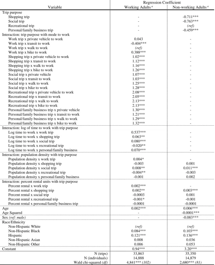
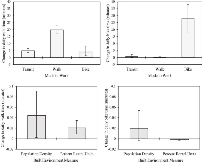
3.3.4. Effect of commuting method and built environment variables on physical activity ... 69
3.3.5.Model validation ... 71
3.3.6.Health impacts of active transportation in the case study region ... 73
3.3.7.Hypothetical HIA application ... 75
3.4. Discussion ... 76
3.4.1.Overall significance ... 76
3.4.2.Comparison to previous studies ... 78
3.5. Limitations ... 79
x
CHAPTER 4: EXPLORING COMPETING TRANSPORTATION HEALTH RISKS AT THE NEIGHBORHOOD SCALE: DEVELOPMENT AND
APPLICATION OF A NOVEL DYNAMIC MICROSIMULATION MODEL ... 82
4.1. Introduction ... 82
4.2. Materials and methods ... 83
4.2.1.Study area ... 85
4.2.2.Demographic data ... 85
4.2.3.Baseline health data ... 87
4.2.4.Exposures ... 88
4.2.4.1. Mobile-source PM2.5 ... 88
4.2.4.2. Transportation physical activity ... 88
4.2.4.3. Motor vehicle, pedestrian, and bicycle crashes ... 88
4.2.5.Health impact model ... 89
4.2.5.1. Baseline transitions ... 90
4.2.5.2. Linking exposures to transition probabilities ... 91
4.2.5.3. Adjustment to avoid double-counting ... 93
4.2.5.4. Health impacts ... 94
4.2.5.5. Model validation ... 94
4.2.6.Neighborhood scale risk comparisons ... 95
4.2.6.1. Built environment measures ... 95
4.2.6.2. Comparisons between groups ... 96
4.3. Results ... 96
4.3.1.VMT regression model ... 96
4.3.2.Health impacts model validation ... 97
4.3.3.Transportation-related exposures ... 98
4.3.4.Transportation health impacts ... 104
4.5. Conclusions ... 115
CHAPTER 5: CONCLUDING REMARKS ... 117
5.1. Key findings ... 117
5.2. Policy implications ... 118
5.3. Limitations ... 121
5.4. Future research ... 124
5.5. Conclusions ... 126
APPENDIX A: SUPPLEMENTARY MATERIAL FOR CHAPTER 2, HEALTH IMPACTS OF INCREASED PHYSICAL ACTIVITY FROM CHANGES IN TRANSPORTATION INFRASTRUCTURE: QUANTITATIVE ESTIMATES FOR THREE COMMUNITIES ... 128
APPENDIX B: SUPPLEMENTARY MATERIAL FOR CHAPTER 3, ESTIMATING ACTIVE TRANSPORTATION BEHAVIORS TO SUPPORT HEALTH IMPACT ASSESSMENT IN THE UNITED STATES ... 140
APPENDIX C: SUPPLEMENTARY MATERIAL FOR CHAPTER 4, EXPLORING COMPETING TRANSPORTATION HEALTH RISKS AT THE NEIGHBORHOOD SCALE: DEVELOPMENT AND APPLICATION OF A NOVEL DYNAMIC MICROSIMULATION MODEL ... 162
xii
LIST OF TABLES
Table 2.1. Relative risks ... 27
Table 2.2. Summary of findings, with 95% confidence intervals based on uncertainty in relative risk parameters ... 33
Table 3.1. Model for estimating daily number of walking trips ... 59
Table 3.2. Model for estimating daily number of biking trips ... 60
Table 3.3. Model for estimating walk trip purpose ... 62
Table 3.4. Model for estimating bike trip purpose ... 63
Table 3.5. Model for estimating walk trip duration ... 66
Table 3.6. Model for estimating bike trip duration ... 67
Table 3.7. Effects of population density on transportation physical activity and estimates of preventable premature deaths relative to the walkable neighborhood counterfactual ... 75
Table 3.8. Transportation physical activity and health benefits estimated for hypothetical built environment changes ... 76
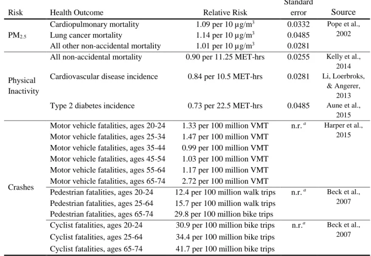
Table 4.1. Relative risk functions (for PM2.5 and physical inactivity) and fatality rates (for crashes) linking exposure to changes mortality risk and disease incidence ... 93
Table 4.2. Regression model for estimating VMT ... 96
Table 4.3. Means and pairwise comparisons of transportation risks between neighborhood groups ... 103
Table 4.4. Means and pairwise comparisons of transportation health impacts between neighborhood groups, year 10 of simulation ... 108
Table A.1. Case study location characteristics ... 131
Table A.2. BRRC focus groups ... 131
Table A.3. Winterville and Sparta meeting participants ... 131
Table A.4. Summary of BRRC focus groups and Winterville and Sparta community meetings ... 132
Table A.5. Baseline disease functions ... 135
Table A.7. Baseline transportation physical activity survey characteristics ... 137
Table A.8. Economic valuation assumptions... 138
Table B.1. Unweighted descriptive statistics, person data ... 142
Table B.2. Unweighted descriptive statistics, active trips (NHTS only) ... 143
Table B.3. Walk trip count models specification tests, from Long and Freese countfit command ... 145
Table B.4. Bike trip count models specification tests, from Long and Freese countfit command ... 146
Table B.5. Average marginal effect daily walk and bike trip count models ... 148
Table B.6. Baseline five-year (2009-2013) average deaths per 100,000 persons, by age, sex, and county ... 152
xiv
LIST OF FIGURES
Figure 1.1. Dynamic and static modeling approaches are first compared (Objective 1), exposure to transportation-related health risks are estimated (Objective 2), and novel health impacts model is used to estimate transportation health impacts for different types of
neighborhoods (Objective 3) ... 16
Figure 1.2. Population density in the study region, illustrating multiple nodes of relatively dense development surrounded by large areas of
low- to moderate-density development ... 17
Figure 2.1. DYNAMO-HIA model schematic representing simulation of one time step. Each circle represents a population state. Solid lines represent possible transitions between states at each time step, whereas dotted lines represent staying in the same state during a time step.
The variables P1-P9 represent transition probabilities between states ... 24 Figure 2.2. Estimated health impacts per 1,000 persons for each community
(solid lines), with 95% confidence intervals reflecting uncertainty
in relative risk parameters (dashed lines) ... 32
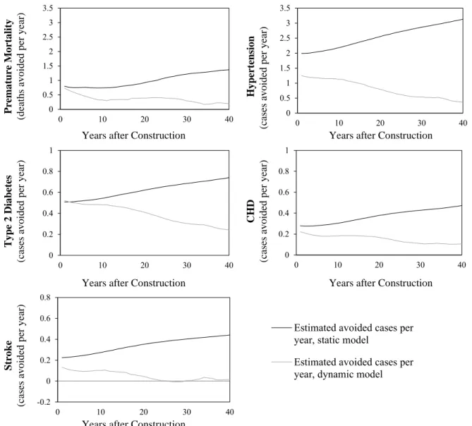
Figure 2.3. Estimated health impacts per year obtained using the HEAT (static) model (solid black lines) and DYNAMO-HIA (dynamic) model
(solid grey lines) for the BRRC case study ... 35
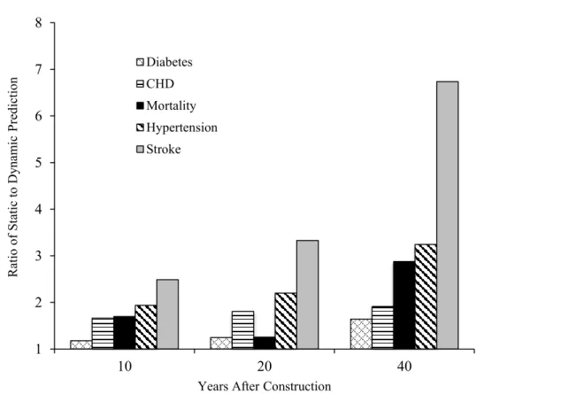
Figure 2.4. Ratio of cumulative health impact estimates from HEAT (static) and DYNAMO-HIA (dynamic) models at 10, 20, and 40 years
after construction ... 37
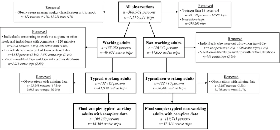
Figure 3.1. Flowchart illustrating data cleaning and stratification of the 2009
NHTS dataset into working and non-working adults ... 49
Figure 3.2. Regression estimates of daily walking and biking time as a function of age, population density, and percent rental units. In each plot,
median values are used for all other variables ... 68
Figure 3.3. Effects of commuting method on daily time spent walking (top left) and biking (top right) relative to the reference category (driving a private vehicle to work), and effects of one-unit changes in built environment measures on daily walking (bottom left) and biking
(bottom right) time ... 70
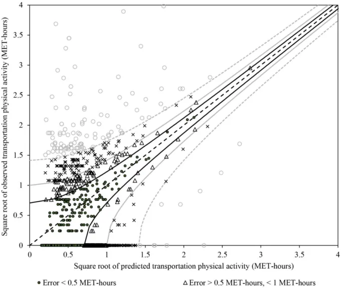
Figure 3.4. Predicted versus observed transportation physical activity for the validation dataset. Dashed black line: perfect agreement. Solid black lines and circular markers: predictions within 0.5 MET-hours per day of observed values. Solid grey lines and triangular markers:
predictions within 1 MET-hour per day of observed values. Dashed grey lines and x-shaped markers: predictions within 2 MET-hours per day of observed values. Hollow circle markers: predictions more than
Figure 3.5. Study region population density (top left), proportion of commuters walking or biking to work (top right), estimated weekly
transportation physical activity (bottom left), and preventable mortality per 100,000 people in 2013. Special districts indicated
in the maps include an international airport and a state park ... 74
Figure 4.1. Individual-level exposure estimates are combined with demographic, health, and relative risk information to estimate health impacts at the individual level using a dynamic microsimulation model and these
estimates are aggregate to explore population-scale health impacts ... 84
Figure 4.2. Population density in the study region, illustrating multiple nodes of relatively dense development surrounded by large areas of low- to
moderate-density development ... 85
Figure 4.3. Population states (h, cvd, and d), mortality states (m1-6), and transition
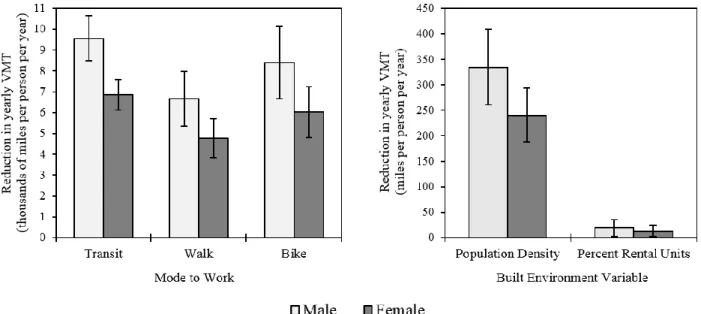
probabilities 𝑃𝑖(𝑆 → 𝑆′) in the Markov chain health impacts model ... 90 Figure 4.4. Average marginal effects (reductions) of a change in mode to work
(left) and a one-unit change in built environment variables (right)
on yearly VMT for women and men... 97
Figure 4.5. Model predicted values (solid lines) versus observed data (markers) for diabetes and CVD prevalence (left) and log-transformed death
rates for men and women (right) ... 98
Figure 4.6. Distribution of PM2.5 from automobiles (top left), transportation
physical activity (top right), per capita yearly VMT (middle left), walk trips (middle right), and bike trips (bottom left). For all
exposures, darker coloring indicates high risk ... 100
Figure 4.7. Neighborhood groups (LW, MLW, MW, MHW, and HW) defined
by quintiles of the walkability index ... 101
Figure 4.8. Box plots illustrating the distributions of each transportation health
risk within the LW, MLW, MW, MHW, and HW neighborhood groups ... 102
Figure 4.9. Estimated cumulative mortality (top left) and excess cases of CVD and diabetes (top right) per 100,000 persons and excess deaths (bottom left) and new cases of CVD and diabetes bottom right) per year per 100,000 persons in the study region associated
with transportation health risks ... 105
Figure 4.10. Mean excess death rates (premature deaths per 100,000) associated with transportation health risks in each neighborhood group 5, 10,
and 20 years from the beginning of the simulation ... 107
Figure 4.11. Cumulative cases of CVD (top left) and diabetes (top right) per 100,000 persons avoided over time and number of new cases of CVD (bottom left) and diabetes (bottom right) per year per 100,000 persons
xvi
Figure 4.12. Attributable mortality rates by transportation risk and mode to work. Negative attributable mortality rates indicate health benefits
relative to the counterfactual scenario (i.e., baseline physical
activity exceeding 37.4 minutes per week) ... 110
Figure 4.13. Transportation-related death rates (left four groups of columns) and excess cases of CVD and diabetes per year (right two groups of columns) by age group ... 111
Figure A.1. Winterville existing pedestrian facilities (left) and proposed improvements (right) ... 128
Figure A.2. BRRC existing open spaces and trails (left) and proposed open space, trails, and improved sidewalks (right) ... 129
Figure A.3. Sparta proposed downtown streetscape improvements ... 130
Figure A.4. Case study population distributions ... 133
Figure A.5. Economic valuations over time ... 139
Figure B.1. Distribution of non-zero observed walk and bike trips counts and descriptive statistics showing little evidence of overdispersion for non-zero counts ... 141
Figure B.2. Comparison of model error (predicted probability minus observed) for each model form (Poisson, negative binomial, and zero-inflated Poisson) for walk and bike trip count models for working adults and non-working adults ... 144
Figure B.3. Predicted probabilities of weekly walk and bike trips. Solid black lines illustrate predicted probabilities and observed trip counts are represented by the dashed black line ... 147
Figure B.4. Average marginal effects of commute mode to work on the probability that a given trip is for one of five purposes (listed across the bottom axis) by race/ethnicity relative to the reference group (private automobile to work) ... 149
Figure B.5. Average marginal effects of trip purpose on walk trip duration for four trip purposes (listed across the bottom axis) relative to work trip duration, by commute mode to work and race/ethnicities ... 150
Figure B.6. Average marginal effects of trip purpose on bike trip duration for four trip purposes (listed across the bottom axis) relative to work trip duration, by commute mode to work and sex ... 151
Figure B.7. Predictions of typical weekday walk trips for a non-Hispanic Black working adult living in the example block group ... 154
Figure B.9. Predictions of weekday walk trip durations by purpose for a non-Hispanic Black working adult who takes transit in work
living in the example block group ... 157
Figure B.10. Predictions of weekday walking time by commute mode to for a non-Hispanic Black working adult who takes transit in work
living in the example block group ... 158
Figure B.11. Distribution of population for males and females in the example block group ... 159 Figure B.12. Distribution of population race for males in the example block group ... 160 Figure B.13. Distribution of commute mode to work, including non-workers,
for a White male in the example block group ... 160
Figure C.1. Estimates of transition rates into the labor force for men (left) and women (right) ... 162
Figure C.2. Estimates of prevalence (top left panel), incidence (top right panel),
and 𝑅𝑅𝑚,𝑑|𝑑 for CVD and diabetes for women, obtained using DisMod II ... 163
Figure C.3. Estimates of prevalence (top left panel), incidence (top right panel),
xviii
LIST OF ABBREVIATIONS
ACS American Community Survey
BRFSS Behavioral Risk Factor Surveillance System BRRC Blue Ridge Road Corridor
CDC Centers for Disease Control and Prevention
CHD Coronary heart disease
CI Confidence interval
CVD Cardiovascular disease
DOT Department of Transportation
DYNAMO-HIA Dynamic Model for Health Impact Assessment
DOT Department of Transportation
EPA Environmental Protection Agency
GEE General estimating equations
GLM Generalized linear models
HEAT Health Economic Assessment Tool
HIA Health impact assessment
HW High walkability
LW Low walkability
MET Metabolic equivalent
MHW Medium-high walkability
MLW Medium-low walkability
MW Medium walkability
N Sample size
NEPA National Environmental Policy Act
OR Odds ratio
P Probability
PA Physical activity
PEF Pedestrian environment factor PM2.5 Fine particulate matter
RR Relative risk
SES Socio-economic status
TPA Transportation physical activity
US United States
USDOT United States Department of Transportation
VMT Vehicle-miles travelled
xx
LIST OF SYMBOLS
𝑨𝑭𝑻𝑷𝑨 Fraction of mortality avoidable by additional active transportation(unitless)
𝑨𝑴𝑻𝑷𝑨 Avoided mortality due to active transportation(avoided premature deaths)
𝑫𝑹𝒃 Baseline death rate(deaths per year per 100,000 persons)
𝑬(𝒕𝒎,𝒊) Expected daily number of trips take using mode m for individual i (trips)
µg/m3 Micrograms per cubic meter
𝜷 Regression coefficient (unitless)
dp,m Trip duration for a trip taken by individual i for purpose p using mode m (minutes) 𝑫𝒔,𝒃𝒆𝒇𝒐𝒓𝒆 Density of sidewalks before construction (km/km2)
𝑫𝒔,𝒂𝒇𝒕𝒆𝒓 Density of sidewalks before construction (km/km2)
𝒇𝒆𝒔𝒕(𝑻𝑷𝑨) Current probability distribution of transportation physical activity (MET-hrs/week)
𝒇𝒄𝒇(𝑻𝑷𝑨) Probability distribution of transportation physical activity in the counterfactual scenario (MET-hrs/week)
𝑶𝒘,𝒃𝒆𝒇𝒐𝒓𝒆 Odds of walking given the density of sidewalks before construction (unitless)
𝑶𝒘,𝒂𝒇𝒕𝒆𝒓 Odds of walking given the density of sidewalks before construction (unitless)
𝝅𝒊 Probability that daily walk or bike trip counts always equals zero (unitless)
𝑬(𝒕𝒎,𝒊) Expected daily number of trips take using mode m for individual i (trips)
𝒈(𝒙) Link function (unitless)
𝑷𝑺,𝑴,𝒕𝒊𝒎𝒆−𝟏 Modeled prevalence of state S in the previous time step in a model with no intermediate disease pathways (unitless)
𝑷𝑺,𝑴+𝑫,𝒕𝒊𝒎𝒆−𝟏 Modeled prevalence of state S in the previous time step in the adjusted model (unitless)
Pr(pm) Probability that a trip taken by individual i using mode m is for purpose p (unitless) 𝑷𝒓 (𝒚𝒊 = 𝒑) Probability of trip purpose p for individual I (unitless)
𝑷𝒊(𝑺 → 𝑺′) Probability that individual i transitions from state S to state S’ during a time step 𝑷𝒘,𝒃𝒆𝒇𝒐𝒓𝒆 Probability that an individual takes at least one walk trip per week before
𝑷𝒘,𝒂𝒇𝒕𝒆𝒓 Probability that an individual takes at least one walk trip per week after construction (unitless)
𝑹𝑹𝑴(𝑻𝑷𝑨) Relative risk of all-cause mortality as a function of transportation physical activity (unitless)
𝑹𝑹𝑴(𝑷𝑴) Relative risk of all-cause mortality as a function of transportation PM2.5 (unitless)
𝑹𝑹𝑺′|𝒆𝒙𝒑𝒐𝒔𝒖𝒓𝒆𝒓,𝒊 Relative risk of state S’ occurring for individual i given exposure to risk r. activity i
(unitless)
𝑻𝑷𝑨𝒊 Daily physical activity from walking and biking for individual i (minutes)
𝑻𝑻𝒎,𝒊 Daily minutes spent traveling using mode m for individual i (minutes) 𝒙 Vector of regression coefficients (unitless)
𝒁𝑭𝑨𝑹 Z-score for retail floor area (unitless)
𝒁𝒊𝒏𝒕𝒆𝒓𝒔𝒆𝒕𝒊𝒐𝒏 Z-score for the number of intersections divided by land area (unitless)
𝒁𝒍𝒂𝒏𝒅−𝒖𝒔𝒆 Z-score land-use diversity (unitless)
1
CHAPTER 1: INTRODUCTION
1.1. Overview of this research
Characteristics of the built environment have a well-documented link to transportation behavior.
The mix of different land uses, the density of land use, access to destinations, physical design, and
availability of public transit services affect the number of trips individuals take, the choice of
transportation mode for trips, and characteristics of trips themselves, such as trip length (Ewing &
Cervero, 2010). In turn, these transportation choices and trip characteristics impact air quality via
emissions from automobiles, physical activity levels via transportation walking and biking, and exposure
to injury risk from crashes for all transportation modes. Today, physical inactivity is associated with
234,000 premature deaths per year in the US (US Burden of Disease Collaborators, 2013). Fatal injuries
from crashes result in an additional 32,000 annual US deaths (US Burden of Disease Collaborators,
2013). Exposure to ambient air pollution is associated with an additional 108,000 annual premature
deaths, nearly half of which are associated with fine particulate matter (PM2.5) emitted by motor vehicles
and other mobile pollution sources (US Burden of Disease Collaborators, 2013; Caiazzo et al., 2013).
These three health risks related to transportation systems—air pollution exposure, physical inactivity, and
fatal injuries from crashes—are linked to both characteristics of the transportation system itself as well as
characteristics of the built environment that influence transportation choices. While the built environment
affects travel behavior, and transportation behaviors impact public health, decisions about transportation
systems and the built environment rarely consider health impacts beyond those associated with traffic
accidents.
The interplay between transportation systems and built environment characteristics results in
emissions are distributed across urban areas in idiosyncratic manners defined by the shape and extent of
the roadway network and commuting patterns within a city. Individuals living near major roadways are
thus exposed to higher levels of air pollution than other residents (Spira-Cohen et al., 2010). Compact
neighborhoods support increased walking and biking for transportation, yet may increase health risks
from air pollution (Hankey, Marshall, & Brauer, 2012). Limited methods currently exist to untangle the
competing effects of transportation health risks in urban areas at the population level. Models considering
a single individual or sub-populations have shown that the health benefits of transportation physical
activity can outweigh other risks. For example, Woodcock et al. demonstrated that physical activity
benefits to individuals using the London bike share system outweighed risks associated with accidents
and air pollution exposure (2014). Population-level models have typically relied on coarse spatial
characterization of exposures to quantify risk (Woodcock et al., 2009; Maizlish et al., 2013). In addition,
population-scale models typically have considered only a single point in time (Mueller et al., 2015).
Given the spatial heterogeneity and dynamic nature of transportation health risks in urban areas,
models that are able to provide dynamic estimates at high spatial resolution are important in untangling
competing risks. This research develops and applies a novel dynamic microsimulation model to estimate
population-level health impacts of transportation systems at high spatial resolution. This model will
support future assessments of transportation health impacts, help improve understanding of the
interactions between the built environment and public health, and could be used to incorporate health
considerations into routine decision-making practices that share transportation system and the built
environment. This research is structured around three objectives:
Objective 1: Apply a dynamic health impact model to estimate the health impacts of increases in
transportation physical activity after a change in the built environment, and compare estimates
from the dynamic model to estimates from a traditional static model.
Objective 2: Develop and demonstrate a statistical model for characterizing baseline
3
from the 2009 National Household Travel Survey to data routinely collected in the American
Community Survey.
Objective 3: Develop and demonstrate a novel dynamic microsimulation health impact model to
estimate population-level health impacts of automobile emissions, physical activity, and fatal
crashes at the Census block group scale.
1.2. Historical perspective
A brief review of historical links between public health and urban planning and the subsequent
divergence of these disciplines along with the suburbanization of US metropolitan areas provides context
for this research. In its formative stages, the field of public health placed a strong emphasis on the built
environment as a risk for poor health. The sanitation movement, a formative force in the
professionalization of public health in the late 19th century, attributed poor health to poor sanitation
conditions based on the theory that foul odors were the mechanism for disease transmission (the “miasma
theory”). As the sanitation movement spread in the US public health departments were increasingly
tasked with urban sanitation (Andrews, 2006). Scientific advancements, specifically the discovery of
microbial pathogens as the mechanism for disease transmission, invalidated the miasma theory that had
formed the basis of early sanitation-focused public health efforts. Subsequently, public health shifted its
focus away from urban planning and toward disease prevention through individual-level interventions,
such as vaccination. By 1925, less than 25% of US cities tasked their public health departments with
urban sanitation (Melosi, 1980).
As the focus of public health shifted towards individual-level disease prevention during the 20th
century, new environmental health risks were emerging in US cities. The industrialization of US cities
brought new urban air quality problems. Lacking a federal regulatory structure to manage air quality,
Industrial emissions were often considered within a common-law framework; however, the courts often
considered the benefits of industrial activities that generated emissions alongside the harms caused by
pollutants (Andrews, 2006). While some cities adopted local air pollution controls, often such policies
statewide efforts to regulate air quality emerged as well; however, these regulatory frameworks were
generally weak (Tarr, 1985). Common-law precedent, the ability of industry to relocate to avoid local
emissions regulations, and the role of upwind pollutions sources made early state and municipal efforts to
manage air quality difficult to implement (Tarr, 1985). These difficulties were in stark contrast to the
success of the urban sanitation movement, which required actions by municipal governments and had
easily identifiable benefits. Air pollution regulations required action by firms and had less discernible
immediate benefits. However, in the wake of highly visible air pollution events, federal air quality
regulations coalesced in the mid-20th century, building to the passage of the Clean Air Act and subsequent
amendments. Implementation of the Clean Air Act greatly improved air quality in cities and further
reduced health risks in urban areas (Melosi, 1980). Subsequent environmental regulations on automobile
emissions and vehicle efficiency further improved air quality in urban areas (EPA, 2011).
While public health shifted towards a more individual-centered approach and environmental
regulations coalesced to address emerging air pollution health risks in US cities, substantial changes in
urban development patterns were occurring. Suburbanization began in the US in the 19th century as
wealthy enclaves began to emerge outside of central cities, enabled by transportation innovations such as
the invention of the streetcar (Fishman, 1989). Interestingly, the same factors that brought about the
sanitation movement motivated early suburbanization, at least in part. For example, the first planned
community in the US, Riverside, Illinois, was designed by two prominent landscape architects of the day,
Frederick Law Olmsted and Calvert Vax, and shared many design characteristics with their grand urban
parks. This development was marketed as a means to have the conveniences of urban life along with the
healthy environment of country living (Kirkman, 2010).
A second transportation innovation—mass production of the Model T—made automobile
ownership affordable to many Americans starting in the 1910s. Investment in infrastructure to support
this new form of mobility quickly followed. Federal aid was first provided for roadway construction in
1916; by 1929, nearly all states in the US had levied gasoline taxes to fund roadway construction
5
ownership. The Federal Housing Authority was created in 1934 and tasked with reinsuring mortgage
loans to make them more affordable (Andrews, 2006). The GI Bill, passed in 1944, further subsidized
home ownership for returning veterans from the Second World War. In 1950, construction began on more
than one million single-family homes in the US (Melosi, 1980). In 1951, the construction of Levittown,
NY, demonstrated how mass production principles could be applied to urban development, providing the
foundation for a fundamentally different urban form than previously existed in the US. In 1956, the
Federal Highway Act pledged the federal government to build a 42,500-mile interstate highway system
(Andrews, 2006). Transportation innovations enabling greater personal mobility through use of
automobiles, substantial investment in infrastructure to support this new form of transportation, and
financial incentives for homeownership provided a suite of complementary forces supporting large-scale
suburbanization in the US.
In contrast to rapid growth of the suburbs, US urban areas were in decline during much of the 20th
century. The Federal Housing Authority was granted the power to differentiate loan guarantees based on
perceived risk. In practice, this power was often used to make federal loan guarantees difficult, if not
impossible, to obtain in neighborhoods with high proportions of minority populations and older housing
stock, a process known as redlining (Jackson, 1985). Redlined urban neighborhoods languished while
many wealthier urban residents moved to the suburbs. Declining urban tax bases made it difficult for
municipal governments and urban school districts to provide quality services. In contrast, suburban
governments and schools reaped the benefits of suburbanization in their own districts. School quality is a
primary driver of household location choice (Bayoh, Irwin, & Haab 2006). Thus, the coupled process of
suburban growth and urban decline was, to some degree, self-reinforcing.
The new urban forms emerging in suburban America differed markedly from traditional urban
development patterns. Land-use regulations rooted in nuisance claims in dense urban environments
coalesced into broader regulations segregating incompatible land uses. Suburban areas were developed on
new sites; however, the same adherence to strict use-based zoning was often applied to suburban
in dense urban areas in low-density developments on new land led to highly segregated land uses—a
characteristic of the built environment that is associated with increased driving, reduced walking and
cycling, and increased trip generation (Ewing & Cervero, 2010).
With the rise of the suburbs and the decline of urban neighborhoods, large shifts were occurring
in health risks related to the built environment. Environmental regulations, motivated by public health
goals, reduced emissions from point-sources. However, increases in vehicle-miles travelled introduced
new air quality issues in cities like Los Angeles. Over time, stricter regulations for motor vehicles helped
address poor air quality from automobiles (Andrews, 2006). However, other health risks increased over
this period. Increased per capita VMT has caused fatality rates from automobile crashes to remain high
despite substantial improvements in vehicle safety and increased efficacy of seat belt laws (Litman,
2014). Today, Americans drive an average of 9,600 miles per year, an increase of over 300% since
1950—the same year in which construction began on more than one million single-family homes
(USDOT, 2016).
1.3. Transportation health risks today
With the fundamental shifts in urban form, environmental regulations, and travel behavior that
occurred in the 20th century, the nature of health risks in US urban areas changed dramatically. While
suburban areas offered an escape from the historically polluted cities, the low-density development and
segregated land-use patterns that typified suburban America did not support walking and biking for
transportation. As environmental regulations evolved and urban air quality improved, health risks in
urban neighborhoods declined. However, emerging health risks from increased automobile dependence
remained or worsened. These broad changes in urban form and environmental quality have generated
complex spatial distributions of competing transportation health risks in urban areas. Not only do these
risks respond to built environment variables in different directions and with different magnitudes, but the
nature of risk-risk tradeoffs is temporally dynamic. Further, transportation health risks may also
disproportionally impact population with low socio-economic status (SES). Historically, the fields of
7
fields diverged at the same time as transportation systems and the built environment changed in ways that
created new health risks. Possibly as a result of the current separation of urban planning and public health,
health-based regulatory frameworks to address the multiple risks that arise from modern urban and
transportation systems have yet to emerge.
Although a regulatory framework for substantively considering the health implications of
transportation and built environment decisions is lacking, urban and transportation planners are
increasingly interested in incorporating health considerations into built environment decisions. Policy
frameworks have emerged in both local and state-level transportation agencies (USDOT, 2012; USDOT,
2014). Health impact assessment (HIA), a structured process for incorporating health considerations into
decision-making, is gaining prominence in the transportation sector (Dannenberg et al., 2014). However,
lacking a compulsory regulatory framework, HIAs are conducted on a largely ad hoc basis. Health-based
standards do interact with transportation decision-making in certain cases. For example, air pollution
exposure is a more routine consideration, including established processes for hotspot analysis triggered
when a region is in violation of national ambient air quality stands (EPA, 2013). In nonattainment areas,
the Congestion Mitigation and Air Quality Improvement Program also provides funds for projects to
reduce transportation emissions; however, these funds make up only a fraction of transportation funding
and are available based on air pollution risks (USDOT, 2016). For crash injury risk, transportation
decision-making often considers VMT exogenous in making decisions about road safety, focusing on
reducing traffic fatalities per VMT rather than traffic fatalities per person. Thus, increases in per capita
VMT due to automobile-dependent urban forms may nullify health gains that would otherwise occur due
to increasing vehicle safety (Litman, 2014).
1.4. Air pollution exposure
1.4.1 Health risks of air pollution exposure
Convincing epidemiological evidence links exposure to ambient air pollutants to a range of health
impacts. Epidemiological studies that consider acute air pollution exposure (e.g., daily or hourly pollutant
respiratory symptoms in response to higher daily PM2.5 concentrations (Brook et al., 2010). Conversely,
epidemiological studies that consider chronic air pollution exposures (e.g., annual average concentrations)
typically assess mortality outcomes, such as increased risk of lung cancer mortality (Pope et al., 2002).
While both acute and chronic exposure to a number of individual pollutants have demonstrated links to
health outcomes, chronic exposure to PM2.5 has an especially strong link to cardiopulmonary and lung
cancer mortality (Pope et al., 2002). Recent scientific reviews conducted by the EPA have concluded that
long-term exposure to PM2.5 is causally linked to increased mortality (EPA, 2012; EPA, 2009).
Interestingly, the effects of long-term exposure to pollutants in ambient air on disease risk is not well
understood despite strong links to cause-specific mortality outcomes in large US cohort studies.
Urban air contains a mixture of airborne pollutants. While each pollutant may pose some health
risk, multi-pollutant risk assessments typically find substantially higher health impacts for PM2.5 exposure
relative to other air pollutants (US Burden of Disease Collaborators, 2013). A recent assessment of
mortality associated with PM2.5 and ozone exposure in the ten most populous US counties found that most
of the risk for premature mortality was associated with exposure to PM2.5 (Fann et al., 2011). Because of
the consistently high health impacts of PM2.5 relative to other pollutants in ambient air, the use of PM2.5 as
a surrogate measure of air quality is common in quantitative risk assessments of air pollution exposure
(e.g., MacDonald Gibson, 2013).
1.4.2 Air pollution exposure and the built environment
A large body of work has investigated the connections between characteristics of the built
environment and air quality. Broadly, this body of evidence can be divided into two categories:
inter-urban studies that compare aggregate built environment measures to average air pollution concentrations
between cities and intra-urban studies that compare neighborhood-scale built environment features to air
pollution concentrations within a single city. In inter-urban studies, more compact urban forms are often
associated with improved air quality (Bereitschaft & Debbage, 2013; Clark et al., 2011). However,
intra-urban variations in air quality suggest an opposite relationship—compact neighborhoods often have
9
Marshall, & Brauer, 2012; Hoek et al., 2011; Moore et al., 2007; Ross et al., 2007; Schweitzer & Zhou,
2010). While compact urban forms are associated with reduced total pollutant mass emissions, compact
neighborhoods may be located in closer proximity to transportation corridors and thereby suffer from
decreased air quality (Spira-Cohen et al., 2010).These effects may be countered via improved vehicle
efficiency (e.g., hybrid/electric vehicles or stricter emissions controls); however, studies reaching such
conclusions often assume aggressive uptake of these technologies in the vehicle fleet (Song et al., 2008).
Previous research has also revealed relationships between poor air quality and indicators of low
SES (Abel & White, 2011; Briggs et al., 2008; Grineski et al., 2013; Buzzelli & Jerrett, 2007; Hajat et al.,
2013).For example, in neighborhoods near the Port of Long Beach, parcels with high concentrations of
mobile-source PM2.5 are more likely to have a high percentage of minority populations (Houston et al.,
2014).A study of neighborhood-scale exposure to NO and O3 in Vancouver, B.C., reached similar
conclusions (Marshall et al., 2006). De Ridder et al. found more sprawling future development would
increase exposure to O3 and PM10 for individuals living in core urban areas but decrease exposure for
those who move from core urban areas to new developments in the urban periphery (2008).A study using
high-resolution air quality estimates in Detroit found that mortality and asthma risks from PM2.5 exposure
were significantly higher in vulnerable than in less-vulnerable populations (Fann et al., 2011). In sum, the
spatial distribution of air pollution risks is complex, is associated with built environment characteristics,
and may affect vulnerable populations disproportionately.
1.5. Physical inactivity
1.5.1. Health risks of physical inactivity
A growing body of evidence links physical activity to a range of health outcomes, including
cardiovascular disease, diabetes, cancers, and all-cause mortality (Aune et al., 2015; Robsahm et al.,
2013; Zhong et al., 2015; Kelly et al., 2014). In addition to studies linking total physical activity to health
outcomes, a subset of studies has documented a preventive relationship between health outcomes and
physical activity accrued specifically from transportation (i.e., walking and cycling for transportation)
exposure to PM2.5 and physical inactivity can affect similar health outcomes, including mortality risks
from pulmonary and cardiovascular diseases as well as all-cause mortality.
1.5.2. Physical inactivity and the built environment
Multiple studies have demonstrated that characteristics of the built environment influence
walking and biking for transportation (Ewing & Cervero, 2010; Bauman et al., 2012). Such studies have
used both stated (i.e., collected via surveys) and objectively measured (e.g., with pedometers) physical
activity (Hirsh et al., 2013; Cerin et al., 2014). Further, studies have shown that built environment
features that encourage transportation physical activity do so independently of effects on recreational
activity—that is, that increases in transportation physical activity associated with more walkable
neighborhoods to not lead to offsetting reductions in recreational physical activity (Ding & Gebel 2012;
Bauman et al., 2012). In addition, studies have shown that a positive relationship between built
environment characteristics and physical activity remains when self-selection (i.e., households sorting
into neighborhoods that match their preferences for physical activity) is introduced as a control in
statistical models (Beenackers et al., 2012; Ding et al., 2012; Saelens et al., 2012; Sallis et al., 2009;
Badland et al., 2012). Longitudinal studies also reveal a positive relationship between built environment
factors and physical activity after controlling for other factors (Giles-Corti et al., 2013). Additionally, a
recent study in Charlotte, NC, compared health outcomes before and after the construction of a light rail
line using a propensity score matching approach and showed that changing one’s commute to light rail
increased physical activity and reduced the risk of obesity (MacDonald et al., 2010).
A complicating factor in the literature is the potential presence of a non-additive, “sum greater
than the parts” relationship between built environment factors measured in different dimensions and
physical activity outcomes. That is, high residential population density and increased mixing of different
land uses may increase physical activity independently; however, the joint effect of the two factors may
be greater than the sum of independent effects. To account for such a relationship, a number of studies
have employed multi-dimension walkability indices (Frank et al., 2010). Similarly, WalkScore has been
11
multi-level designs to account for potential interactions between built environment factors at the regional
and neighborhood scales (Clark et al., 2014).Some studies have developed unique neighborhood
typologies using techniques such as cluster analysis to define comparison groups within an urban area
(Zahabi et al., 2013). Although cluster analysis and multi-dimension indices may have more power to
identify significant relationships, they are unable to identify specific built environment factors that
explain observed differences in physical activity levels between neighborhoods. Thus, studies using
cluster analysis have limited generalizability while multi-dimension indices mask the effect of specific
dimensions, such as increased population density holding all else constant, on physical activity. Because
of the complexity of measuring built environment factors associated with walkability, associations
between physical activity and built environment measures depend in part on the specific built
environment measures employed.
Physical activity levels vary significantly between socio-economic groups in the US: in an
analysis of accelerometry data from the 2005–2006 National Health and Nutrition Examination Survey,
African-Americans were 36% more likely to be inactive than European-Americans, and those living in
low-income households were 94% more likely to be inactive than those living in high-income households
(Sisson et al., 2012). While low-SES populations may be more likely to participate in labor-intensive jobs
and depend on public transportation for mobility, high-SES populations may be more likely to engage in
recreational physical activity. Further, evidence suggests that low- and high-SES populations may
respond to neighborhood amenities in different ways: Sallis et al. found that income residents in
low-walkability neighborhoods have higher levels of transportation physical activity than their high-income
counterparts; however, low-income residents in high-walkability neighborhoods have significantly lower
transportation physical activity levels than high-income residents (2009). Other evidence in the literature
is mixed. Wen et al. found that neighborhood factors do not mediate differences in walking by race
(2007).Several studies have also found associations between body mass index, neighborhood design, and
access to public transit (MacDonald et al., 2010; Carlson et al., 2012; Hess & Russell, 2012). However, a
in disadvantaged populations (Pearce et al., 2011). While the evidence is mixed, modifiable built
environment factors may mediate observed health disparities in vulnerable populations. Thus, exploring
the potential mediating effect of the built environment on physical activity has important environmental
justice implications.
1.6. Motor vehicle, bicycle, and pedestrian crashes
1.6.1. Health risks of motor vehicle, bicycle, and pedestrian crashes
Compared to epidemiological studies of air pollution and physical activity health risks,
epidemiological approaches to assessing health risks from crashes are limited by less readily available
data to characterize exposure. For motor vehicle fatalities, exposure is typically characterized by the total
length of travel (e.g., VMT); however, data on walking and biking are much more limited. Thus, studies
that assess risk for pedestrians and cyclists use less refined measures of exposure, such as number of
walking or biking trips (Beck, Dellinger, & O’Neil, 2007). National-level traffic fatality and travel data
have been linked in a number of studies to estimate fatality risk as a function of distance traveled and/or
trips taken by population sub-groups (Harper, Charters, & Strumpf 2015; Beck, Dellinger, & O’Neil,
2007). National-level studies have found evidence of differential risk for some populations, such as higher
crash fatality risk per VMT for younger males who may engage in riskier driving behaviors (Harper,
Charters, & Strumpf, 2015). As an alternative to national-level studies, Grabowski and Morrisey used
state-level data to show that reductions in gas prices and concomitant increases in VMT explain increased
fatality rates (2004). At a more refined spatial scale, a study in San Antonio also revealed a strong
relationship between VMT assessed at the neighborhood scale (census block groups) and fatal crashes
(Dumbaugh & Rae, 2009).
1.6.2. Motor vehicle, bicycle, and pedestrian crashes and the built environment
Built environment factors play a substantial role in modifying the risk for fatal pedestrian and
bicycle crashes but have mixed effects on fatalities from motor vehicle crashes. Area-level studies have
found associations between built environment characteristics and risks for pedestrians and cyclists. For
13
associated with motor vehicle traffic volumes within Census tracts, controlling for other built
environment variables (Gladhill & Monsere, 2012; Wier et al., 2009). Associations have also been
demonstrated between the total number of pedestrians and reductions in individual risk, a phenomenon
known as the safety-in-numbers theory (Jacobsen, 2003). However, the safety in numbers theory has been
criticized because it may be that increased walking and biking are responses to unobserved built
environment factors that reduce risk rather than the mechanism for risk reduction (Bhatia & Wier, 2011).
Conversely, built environment variables, including population density, public transit usage, and
volume-to-capacity ratio on streets, have mixed effects on risk estimates (Clark & Cushing, 2004; Simpson et al.,
2014). While area-level studies are useful in targeting interventions to reduce pedestrian and cyclist
fatalities in high-risk locations, limited conceptualization of individual-level dose (i.e., walk trips per
person) in these studies limits their usefulness in population-level assessments of health risks from traffic
crashes.
From an environmental justice perspective, individuals who rely on active modes of
transportation may be exposed to greater risk compared to individuals with access to a private automobile
for mobility— especially if low-income neighborhoods are less walkable than more affluent
neighborhoods. However, motorists with long commutes may also be exposed to greater risk from motor
vehicle fatalities if fatality risk is a function of VMT. Further, advances in vehicle safety have resulted in
heterogeneity within the vehicle fleet: new vehicles are generally safer than older vehicles (Farmer &
Lund, 2006). The potential for disparities in risk for road injury is great, especially considering recent
trends in the US such as the suburbanization of poverty (Steven & Stoll, 2010). Studies in New York
City; British Columbia, Canada; and Chicago have found significant relationships between road injuries
and indicators of vulnerability, including minority status, education, unemployment, and income
(Ukkusuri, Hasan, & Aziz, 2011; Bell et al., 2012; Cottrill & Thakuriah, 2010). Lower-income
individuals, especially those living in low-walkability, suburban, and/or rural neighborhoods with long
1.7. Frameworks for comparing competing transportation risks
While transportation systems alter health risks through automobile emissions, fatal crashes, and
physical activity, quantitative methods to explore the health implications of these risks are limited.
Hankey, Marshall, and Brauer estimated the relative health impacts of air pollution exposure and physical
activity in Los Angeles (2012). Comparing these two risks, the authors found a nearly one-to-one risk
tradeoff between walkable and non-walkable neighborhoods—that is, while residents of walkable
neighborhoods are exposed to greater air pollution levels, increased physical activity counterbalances
these health risks.. Comparing the health impacts of potential future changes in transportation behaviors,
Woodcock et al. used a multi-risk framework to demonstrate that the health benefits of encouraging
increased transportation physical activity were greater than the benefits of reducing automobile emissions
in San Francisco, London, and Delhi (Maizlish et al., 2013; Woodcock et al., 2009). This same
framework was used to estimate the health benefits to individuals who use the London bike share system
(Woodcock et al., 2014). Replacing short motor vehicle trips with bicycle trips substantially benefited
health for users of the system. Finally, De Nazelle, Rodriguez, and Crawford-Brown developed a
microsimulation framework to assess changes in energy expenditures and pollutant inhalation given
hypothetical changes to the built environment to find that physical activity and air pollution inhalation
may both increase given hypothetical changes to the built environment (2009).
Previous multi-risk frameworks have explored competing transportation risks in urban areas.
However, population-level studies have relied on coarse characterization of exposure (e.g., using large
gird cells to estimate air pollution exposure) (Maizlish et al., 2013; Woodcock et al., 2009). Other studies
have assessed impacts in specific sub-populations, such as users of the London bike share (Woodcock et
al., 2014) or individuals (De Nazelle, Rodriguez, & Crawford-Brown, 2009), but have not estimated
population-level health impacts of transportation systems. Using survey data collected for a large sample
of individuals in Los Angeles, Hankey, Marshall, and Brauer presented a framework that begins to bridge
the gap between individual-level and population-level studies, but this framework does not estimate
Population-15
level estimates of health impacts are useful for exploring the role of the built environment in influencing
transportation health risks, while individual-level studies offer richer understanding of competing health
pathways (e.g., comparing an active to a non-active commuter in a polluted neighborhood). However,
individual-level health impact models have not been used to estimate population-level health impacts
associated with transportation systems. In other sectors, population-level health impacts of interventions
such as smoking cessation and body mass index reduction have been explored using individual-level
microsimulation models (Lhiachimi et al., 2010). In sum, while frameworks to explore competing
transportation health risks have emerged in recent years, no such framework exists for comparing air
pollution, physical inactivity, and fatal injury risk from crashes in a dynamic population-scale model.
This research builds upon previous work assessing the competing health risks of transportation
systems by developing an advanced micro-simulation model and applying the model to estimate
transportation health risks across the Raleigh-Durham-Chapel Hill metropolitan area. This research is
divided into three principal objectives (Figure 1). First, an existing dynamic modeling tool is used to
estimate the health benefits of increased physical activity from transportation in a single neighborhood in
the study region. These estimates are then compare to estimates obtained using a more traditional risk
assessment approach that uses a static calculation of health benefits (Objective 1). Regression models are
then used to predict transportation physical activity at the Census block group geography across the study
region (Objective 2). Then, a novel dynamic multi-risk micro-simulation model tailored to transportation
health risks is developed, combining physical activity, walk and bike trip, VMT, and high-resolution air
pollution estimates. This model is then applied across the study region to estimate transportation health
risks at the Census block group geography. Finally, estimated health risks are compared between
Figure 1.1. Dynamic and static modeling approaches are first compared (Objective 1), exposure to
transportation-related health risks are estimated (Objective 2), and novel health impacts model is used to
estimate transportation health impacts for different types of neighborhoods (Objective 3).
1.8. Study Region
To demonstrate the methods developed in this thesis, the methods are applied to estimate
transportation health risks at the Census block group scale across the Raleigh-Durham-Chapel Hill region.
This region is a large urban agglomeration in central North Carolina. The region has several nodes of
high-density development surrounded by large suburban areas (Figure 2). The region is highly
auto-dependent, with nearly 90% percent of workers commuting using an automobile in 2013 (US Census
17
Figure 1.2. Population density in the study region, illustrating multiple nodes of relatively dense
development surrounded by large areas of low- to moderate-density development.
1.9. Research Significance
Transportation health risks have significant impacts on population health and are distributed in
complex spatial patterns across urban areas. Yet, tools and methods to estimate the health impacts of
transportation systems are poorly developed. Previous studies exploring competing transportation health
risks in urban areas have used coarse estimates of exposure to transportation risks, employed static health
impact models, and focused on individuals or specific sub-populations without translating findings to the
population scale. This research builds upon previous work by characterizing exposure at the individual
level for all members of the population, estimating health impacts at fine spatial resolution to facilitate
neighborhood-level comparisons of risks with built environment factors, and employing an advanced
dynamic microsimulation model. In doing so, this research supports more rigorous consideration of
transportation health risks and offers more detailed understanding of the complex tradeoffs that occur
CHAPTER 2: HEALTH IMPACTS OF INCREASED PHYSICAL ACTIVITY FROM CHANGES IN TRANSPORTATION INFRASTRUCTURE: QUANTITATIVE ESTIMATES FOR THREE
COMMUNITIES1
2.1. Introduction
In the United States, approximately 234,000 premature deaths are associated with physical
inactivity each year (US Burden of Disease Collaborators, 2013). The built environment influences
walking and biking for transportation and, in turn, total physical activity (Ewing & Cervero, 2010;
Bauman et al., 2012). Many communities in the United States are designed in ways that do not support
walking and biking, thereby contributing to low levels of physical activity (Lee, Ewing, & Sesso, 2009).
Recently, transportation agencies across the United States have sought to integrate health considerations
into decision-making (USDOT, 2014; USDOT, 2012). Health impact assessment (HIA) has emerged as a
systematic framework for considering how decisions, such as modifications to the built environment, may
impact public health and has informed a variety of decisions in the transportation sector (National
Research Council, 2011; Wernham, 2013). However, most transportation HIAs conducted to date have
provided qualitative rather than quantitative estimates of health benefits arising from changes in physical
activity (e.g., indicating that physical activity is expected to increase, without estimating the magnitude of
the increase) (Bhatia & Seto, 2011). Existing research links the built environment to physical activity
levels and health outcomes, but quantitative models to predict the health impacts of modifications to the
built environment remain poorly developed (McCormack & Shiell, 2011; MacDonald et al., 2010; Hess &
Russell, 2012).
1 This chapter previously appeared as an article in BioMed Research International. The original citation is
as follows: Mansfield TJ, MacDonald Gibson J. Health impacts of increased physical activity from changes in transportation infrastructure: quantitative estimates for three communities. Biomed Res Int
19
Within the past four years, two new tools to support quantitative HIAs have emerged. The first
tool, the Health Economic Assessment Tool (HEAT) for cycling and walking, was introduced by the
World Health Organization in 2011 (Kahlmeier et al., 2014). More recently, the European Union Health
Programme released the Dynamic Model for Health Impact Assessment (DYNAMO-HIA) (Lhachimi et
al., 2012). These two tools employ fundamentally different methods; while DYNAMO-HIA is dynamic,
capable of tracking changes in population health over many years, HEAT is static, providing health
impact estimates for a single year. The HEAT method has been used in several HIAs of policies or
projects to promote active transportation (walking or cycling instead of driving) (Mueller et al., 2015).
DYNAMO-HIA has been applied to estimate the health impacts of a ban on alcohol imports in Sweden,
smoking cessation in Great Britain, reduced salt intake in Europe, decreased smoking prevalence in
Copenhagen, and body mass index reduction in Netherlands (Lhachimi et al., 2012; Hendriksen et al.,
2015; Holm et al., 2014; Boshuizen et al., 2012). However, to our knowledge, DYNAMO-HIA has not
yet been applied to predict the health impacts of increased physical activity arising from changes in the
built environment. Further, the estimates from these two methods have not been compared.
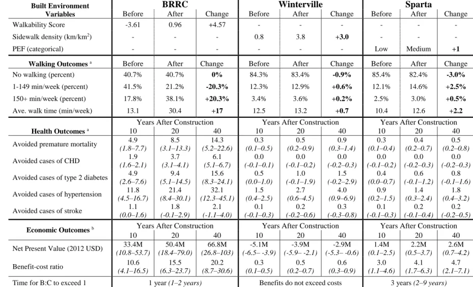
To demonstrate the use of quantitative tools for estimating the health effects of physical activity
in HIAs of the built environment, this paper describes quantitative HIAs of proposed changes to the built
environment in three North Carolina communities. All three HIAs used DYNAMO-HIA to estimate the
health effects of increased transportation walking time expected to arise due to modifications to the built
environment. Changes in premature mortality, coronary heart disease (CHD), type 2 diabetes,
hypertension, and stroke were estimated for each community. In addition, each HIA estimated the ratio of
health benefits to expected project costs. For one of the case studies, we additionally compared results
obtained from DYNAMO-HIA with those obtained from the HEAT model. Our objective in making this
comparison was to determine whether the health impact estimates differ when using a dynamic approach
(as in DYNAMO-HIA) as compared to a static approach (as in HEAT). We hypothesized that the static
approach may overestimate health benefits by failing to account for overall improvements in population
for which no benefits have yet accrued. Our overall purpose was twofold: first, to demonstrate that
quantitative tools in general may provide objective, evidence-based decision support within the HIA
framework and, second, to provide insight into the advantages and disadvantages of emerging quantitative
tools and methods to conduct HIAs.
The HIAs presented in this study were conducted as examples to support WalkBikeNC, a
statewide bicycle and pedestrian plan developed by the North Carolina Department of Transportation
(NCDOT) in 2013 (NCDOT, 2013). WalkBikeNC presents a unified policy framework to support active
travel statewide, but it does not propose projects. Instead, specific bicycle and pedestrian infrastructure
projects are planned and implemented by local authorities in accordance with WalkBikeNC. Such projects
may be included in a range of local plans, including small-area plans, comprehensive transportation plans,
and bicycle and pedestrian master plans. The three HIAs described in this paper consider pedestrian
infrastructure improvements aligned with the policy framework established in WalkBikeNC at three
planning scales: a small-area plan, a comprehensive plan, and a streetscape plan.
2.2 Materials and Methods
All three case studies followed the six steps of HIA proposed by the US National Research
Council: (1) screening; (2) scoping; (3) assessment; (4) recommendations; (5) reporting; and (6)
monitoring and evaluation (National Research Council, 2011). The first two steps of HIA, screening and
scoping, focus on identifying and characterizing health concerns and disparities in the community. The
third step, assessment, explores how the decision to be made influences these concerns and disparities
through qualitative understanding and/or quantitative modeling of causal pathways as understood in the
scientific literature. The conclusions from the assessment stage inform the fourth stage, recommendations.
Finally, reporting and monitoring and evaluation aim to engage stakeholders, hold decision-makers
accountable, and evaluate the effectiveness of the decision in addressing identified health concerns at
some point in the future. Because this paper focuses on improving the assessment stage through the