Throughput Optimization Routing Under Uncertain Demand for Wireless
Mesh Networks
Yuan Xue, Liang Dai, Bin Chang, Yi Cui
Department of Electrical Engineering and Computer Science, Vanderbilt University {yuan.xue, liang.dai, bin.chang, yi.cui}@vanderbilt.edu.
Abstract—Wireless mesh networks have attracted in-creasing attention and deployment as a high-performance and low-cost solution to last-mile broadband Internet access. Network routing plays a critical role in determining the performance of a wireless mesh network. To study the best mesh network routing strategy which can maximize the network throughput while satisfying the fairness con-straints, existing research proposes to formulate the mesh network routing problem as an optimization problem. These works usually make ideal assumptions such as known static traffic input. Whether they could be applied for practical use under the highly dynamic and uncertain traffic in wireless mesh network is still an open issue.
The main objective of this paper is to understand the effects of traffic uncertainty in wireless mesh networks and consider these effects in throughput maximization routing. It identifies the appropriate optimization framework that could integrate the statistical user traffic demand model into a tractable throughput maximization problem. The trace-driven simulation study demonstrates that our al-gorithm can effectively incorporate the traffic demand uncertainty in routing optimization, and outperform the throughput maximization routing which only considers static traffic demand.
I. INTRODUCTION
Wireless mesh networks [1], [2] have attracted in-creasing attention and deployment as a high-performance and low-cost solution to last-mile broadband Internet access. In wireless mesh networks, local access points and stationary wireless mesh routers communicate with each other and form a backbone network which forwards the traffic from mobile clients to the Internet.
Traffic routing in the mesh backbone network plays a critical role in determining the performance of a wireless mesh network. These existing routing solutions usually fall into two ends to the spectrum. On one end of the spectrum are the heuristic algorithms (e.g., [3], [4], [5], [3]). Although many of such approaches are adaptive to the dynamic environments of wireless networks, they lack the theoretical foundation to analyze how well the network performs globally (e.g., whether the network
resource is fully utilized, whether the flows share the net-work in a fair fashion). On the other end of the spectrum, there are theoretical studies that formulate these network planning decisions into optimization problems (e.g., [6], [7]). Yet these results usually make ideal assumptions towards the network such as known static traffic input, which makes them unsuitable for practical use in the highly dynamic wireless networking environments.
To date, how mesh network could optimize its perfor-mance under dynamic user demand is still an open ques-tion. This question calls for a new framework that could characterize the traffic demand uncertainty and integrate its effect into optimal network routing. To answer this call, this paper investigates the traffic routing problem for throughput optimization with fairness constraint under uncertain demand. In particular, it studies how traffic from(to) local access points could be routed in a mesh network so that the minimum proportion of the demands from all local access points could be maximized.
If the traffic demand from each local access point is known a priori, the throughput optimization problem with fairness constraint could be formulated as a lin-ear programming problem (maximum concurrent flow problem). To incorporate demand uncertainty into this optimization framework, this paper first characterizes the uncertain traffic demand using a random variable. Under this model, the proportions of traffic demands are also random variables for a given routing strategy. Thus this paper extends the maximum concurrent flow problem to a stochastic optimization problem where the expected value of the minimum proportion of all traffic demands is maximized. This paper further presents two fast (1−ǫ )-approximation algorithms for throughput optimization under fixed and uncertain demand respectively.
To evaluate and compare the performance of these two algorithms under realistic network traffic environment, we conduct trace-driven simulation study. In particular, we derive the traffic demands from the access points of campus wireless LANs based on the traces collected at Dartmouth College [8]. These traffic demands are used to
drive the simulation. Our simulation results demonstrate that our statistical problem formulation could effectively incorporate the traffic demand uncertainty in routing optimization, and our algorithm outperforms the con-ventional solution which only considers the static traffic demand.
The original contributions of this paper are two-fold. First, to the best of our knowledge, this is the first work that integrates statistical user traffic demand model into a tractable throughput optimization problem for wireless mesh networks. Second, this paper evaluates the practicability of optimization-based routing solutions using the trace data collected in the real wireless network environments.
The remainder of this paper is organized as follows. Sec. II presents the network and traffic demand model. Sec. III formulates the mesh network routing problem under fixed traffic demand based on maximum concur-rent flow and presents a fast approximation algorithm. Sec. IV extends the routing problem to handle uncertain traffic demand. We show simulation results in Sec. V, present related work in Sec. VI and finally conclude the paper in Sec. VII.
II. MODEL
A. Network Model
Internet
gateway access point
clients
mesh node
local access point
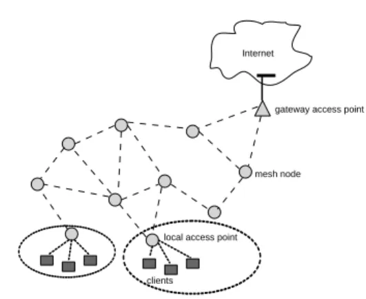
Fig. 1. Illustration of Wireless Mesh Network
We consider a multi-hop wireless mesh network as illustrated in Fig. 1. In this network, local access points aggregate the traffic from mobile clients that are asso-ciated with them. They communicate with each other, also with stationary wireless routers, forming a multi-hop wireless backbone network which forwards the user traffic to a gateway access point connecting to the Internet. In the following discussion, local access point, gateway access point, and mesh routers are collectively called mesh nodes.
We model the backbone of a wireless mesh network as a directed graphG= (V, E), where each nodeu∈V
represents a mesh node. Among these nodes, g ∈ V is the gateway access point that connects to the Internet. A directed edge e = (u, v) ∈ E denotes that u can transmit to v directly. We assume that all mesh nodes have a uniform transmission range denoted by RT. We
denoter(u, v)as the distance betweenuandv. An edge
e= (u, v)∈E if and only ifr(u, v)≤RT. We also use r(e) to represent the length of edge e. Let b(e) bit/sec be the data rate of edgee, which is maximum data that can be carried in a second alonge.
B. Traffic Demand Model
This paper investigates the throughput optimization routing scheme for wireless mesh backbone network. Thus we consider the aggregated traffic among the mesh nodes. In particular, we regard the gateway access points as the source of all incoming traffic and the destination of all outgoing traffic of a mesh network. Similarly, the lo-cal access points, which aggregate the client traffic, serve as the sources of all outgoing traffic and the destinations of incoming traffic. For simplicity, we call the aggregated traffic that shares the same source and destination as a flow and denote it as f ∈ F, where F is the set of all aggregated flows. It is worth noting that although we consider only one gateway access point in this paper, our problem formulation and algorithm presented here could be easily extended to handle multiple gateway routers and inter-mesh-router traffic. Finally, we denote the rate of an aggregated flow f ∈ F as xf, and use
x = (xf, f ∈ F) to represent the aggregated flow rate
vector.
C. Interference Model and Schedulability
In a wireless network, packet transmissions are sub-ject to location-dependent contention, which means that simultaneous transmissions in the proximate region may interfere with each other and result in packet collision. Usually the interference range of a node is larger than its transmission range. Thus we denote the interference range of a node as RI = (1 + ∆)RT, where ∆≥0 is a
constant.
In this paper, we consider the protocol model for packet transmission [9]. In the protocol model, packet transmission from nodeu to v is successful if and only if (1) the distance between these two nodes r(u, v) satisfies r(u, v) < RT; (2) any other node w ∈ V
within the interference range of the receiving node v, i.e., r(w, v) ≤ RI, is not transmitting. Two edges e, e′ interfere with each other, if they can not transmit
simultaneously based on the protocol model. We useI(e) denote the set of edges which interfere with edge e.
To study the throughput optimization routing prob-lem, we first need to understand the constraint of the flow rates. Let y = (ye, e ∈ E) denote the wireless
link rate vector, where ye is the aggregated flow rate
along wireless link e. Link rate vector y is said to be schedulable, if there exists a stable schedule that ensures every packet transmission with a bounded delay. Essentially, the constraint of the flow rates is defined by the schedulable region of the link rate vector y.
The link rate schedulability problem has been stud-ied in several existing works, which lead to different models [10], [11], [12]. In this paper, we adopt the model in [11], which presents a sufficient condition under which a link scheduling algorithm is given to achieve stability with bounded and fast approximation of an ideal schedule. Based on this model, we define S(e) as a subset of I(e) where each e′ ∈ S(e) has a length
r(e′) greater than or equal to r(e). In the following discussion, we refer S(e) as the adjusted interference set of e. Based on the results presented in [11], we have the following claims.
Claim 1. (Sufficient Condition of Schedulability) The
link rate vector y is schedulable if the following condi-tion is satisfied:
∀e∈E, ye+ X
e′∈S(e)
ye′ ≤b(e) (1) where b(e)bit/sec is the data rate of edgee. For ease of exposition, we assume thatb(e) = 1 for alle∈E in the following discussion.
III. FIXEDDEMAND MESHNETWORKROUTING
In this paper, we investigate the throughput opti-mization routing problem for wireless mesh backbone network. The objective of this problem is to maximize the throughput of aggregated flows among local access points and the gateway, while satisfying the fairness constraints. This problem is usually formulated as a maximum concurrent flow problem. In this section, we first study the formulation of throughput optimization routing in wireless mesh backbone network under fixed traffic demand. We then present a fully polynomial time approximation algorithm (FPTAS) for this problem, which finds an ǫ-approximate solution. The problem formulation and algorithm presented in this section serve as the basis of the uncertain demand routing problem discussed in Sec. IV.
Notation Definition
G= (V, E) Network
u∈V Node
g∈V Gateway Router
e= (u, v)∈V An Edge Connecting nodesuandv
f∈F Flow, also known as Commodity
x= (xf, f∈F) Aggregated Flow Rate Vector
y= (ye, e∈E) wireless link flow rate vector
d= (df, f∈F) Flow Demands
Pf Set of Unicast Paths that could Route
Flowf
xf(P) Rate of Flowf over PathP ∈Pf
λ Scaling Factor
Se Interference Set ofe∈E
AeP =|Se∩P| Number of Wireless LinksP passes in
Se
µe Price ofSe
λ(d) = minf∈F{ xf
df} Scaling Factor ford
λ∗ (d) Optimal Value ofλ(d) θ=λ(d)/λ∗( d) Performance Ratio p(d) Probability ofd TABLE I NOTATIONS
Recall that f ∈ F is the aggregated traffic flow between local access points and the gateway. We usedf
to denote the demand of flowf andd= (df, f ∈F) to
denote the demand vector consisting of all flow demands. Consider the fairness constraint that, for each flowf, its throughput being routed is in proportion to its demand
df. Our goal is to maximizeλ(so called scaling factor)
where at least λdf amount of throughput can be routed
for flow f. We assume an infinitesimally divisible flow model where the aggregated traffic flow could be routed over multiple paths and use Pf to denote the set of
unicast paths that could route flow f.
Let xf(P) be the rate of flow f over path P ∈ Pf.
Obviously the aggregated flow rateyealong edgee∈E
is given by ye = Pf:P∈Pf&e∈Pxf(P), which is the
sum of flow rates that are routed through paths P
passing edge e. Based on the sufficient condition of schedulability in Claim 1 (Eq.(1)), we have that
X f:P∈Pf&e∈P xf(P) + X e′∈S e X f:P∈Pf&e′∈P xf(P)≤1 (2)
The throughput optimization routing with fairness constraint is then formulated as the following linear programming (LP) problem:
P: maximize λ (3) subject to X P∈Pf xf(P)≥λdf,∀f ∈F (4) X f:P∈Pf&e∈P xf(P) (5) + X e′∈S e X f:P∈Pf&e′∈P xf(P)≤1,∀e∈E λ≥0, xf(P)≥0,∀f ∈F,∀P ∈ Pf(6)
In this problem, the optimization objective is to maxi-mizeλ, such that at leastλdf units of data can be routed
for each aggregated flow f with demand df. Inequality
(4) enforces fairness by requiring that the comparative ratio of traffic routed for different flows satisfies the comparative ratio of their demands. Thus, the absolute value df is meaningless, as we can easily tune the value
of λ by scaling up/down all demands, while λdf stays
unchanged. Inequality (5) enforces capacity constraint by requiring the traffic aggregation of all flows passing wireless link e ∈ E satisfy the sufficient condition of schedulability. This problem formulation follows the classical maximum concurrent flow problem, which has also been used in Internet traffic engineering and load balancing routing.
This problem could be solved by a LP-solver such as [13]. To reduce the complexity for practical use, we present a fully polynomial time approximation algorithm (FPTAS) for problem P, which finds an ǫ-approximate solution. The key to a fast approximation algorithm lies on the dual of this problem, which is formulated as follows. First we defineAeP =|Se∩P|as the number of
wireless links a pathP passes in the adjusted interference set Se. We assign a price µe to each set Se for e∈E.
The objective is to minimize aggregated price for all adjusted interference sets. As the constraint, Inequality (8) requires that the price Pe∈EAePµe of any path P ∈ Pf for flow f must be at least µf, the price of
flowf. Further, Inequality (9) requires that the weighted flow price µf over its demand df must be at least 1.
D: minimize X e∈E µe (7) subject to X e∈E AePµe≥µf,∀f ∈F,∀P ∈ P(8)f X f∈F µfdf ≥1 (9)
Algorithm I: Mesh Network Routing Under Fixed Demand
1 ∀e∈E,µe←β 2 xf(P)←0, ∀P ∈ Pf,∀f∈F 3 whileP e∈Eµe<1 4 for∀f∈F do 5 d′ f ←df 6 whileP e∈Eµe<1andd′f >0do
7 P ←lowest priced path inPf usingµe
8 δ←min{d′ f,mine∈P A1 eP} 9 d′ f ←d ′ f−δ 10 xf(P)←xf(P) +δ 11 ∀es.t.AeP 6= 0,µe←µe(1 +ǫδAeP) 12 end while 13 end for 14 end for TABLE II
ROUTINGALGORITHMUNDERFIXEDDEMAND
Based on the above dual problem D, our fast ap-proximation algorithm is presented in Table II. The algorithm design follows the idea of [14]. To start with, we initialize the price on each adjusted interference set
Se as β (Line 1). We also zero the traffic on all paths P ∈ Pf (Line 2). Then for each flow f, we route df
units of data. We do so by finding the lowest priced path in the path set Pf (Line 7), then filling traffic to
this path by its bottleneck capacity (Lines 8 to 10). Then we update the prices for physical edges appeared in this path based on the function defined in Line 11. We keep filling traffic to flow f in the above fashion until all
df units are routed. This procedure is repeated until the
aggregate price of interference sets Se for all e ∈ E
weighted by the capacity cexceeds 1 (Line 3).
We make following notes to our algorithm. First, it completes in finite time, which is guaranteed by the asymptotic link price update function defined in Line 11. ǫ here is the step size, which controls the growing speed of the link price. Second, as one might see, the algorithm in fact routes more traffic than the network is able to afford. Therefore, a scaling procedure is needed to scale down the routed traffic so it fits the capacity of each physical link in the network. We formally analyze the properties of our algorithm in the following lemmas and theorem. In the analysis, we denotef∗ as the result
returned by the algorithm andOP T as the optimal value ofD as well as P.
Lemma 1: If OP T ≥ 1, scaling the final flow by
log1+ǫ1/β yields a feasible primal solution of value
f∗ = t−1
log1+ǫ1/β, t being the number of phases the
algorithm takes to stop.
Lemma 2: If OP T ≥ 1, then the final flow scaled
when β= (|E|/(1−ǫ))−1/ǫ.
Lemma 3: If OP T ≥ 1 and β = (|E|/(1 −
ǫ))−1/ǫ, Algorithm I terminates after at most t = 1 + OP Tǫ log1+ǫ 1|E−|ǫ phases.
These lemmas require that OP T ≥ 1. The running time of the algorithm also depends on OP T. Thus we need to ensure that OP T is at least one and not too large. Let ζf be the maximum traffic value of flow f
when all other flows have zero traffic. Let ζ = minf ζdff.
Since at best all single commodity maximum flows can be routed simultaneously,ζ is an upper bound onf∗. On the other hand, routing 1/|F| fraction of each flow of value ζf is a feasible solution, which implies thatζ/|F|
is a lower bound on OP T. To ensure that OP T ≥ 1, we can scale the original demands so that ζ/|F| is at least one. However, by doing so, OP T might be made as large as |F|, which is also undesirable.
To reduce the dependence on the number of phases on OP T, we adopt the following technique. If the algorithm does not stop after T = 2ǫlog1+ǫ 1|E−|ǫ phases, it means that OP T >2. We then double demands of all commodities, so that OP T is halved and still at least 1. We then continue the algorithm, and double demands again if it does not stop after T phases.
Lemma 4: Givenζf for each flowf, the running time
of Algorithm I is O(logǫ2|E|(2|F|log|F|+|E|))·Tmp.
Theorem 1: The total running time of Algorithm I
is O(ǫ12[log|E|(2|F|log|F|+|E|) + logU)])·Tmp.
We delay proofs to the above lemmas and theorem to the appendix.
IV. UNCERTAINDEMANDMESH NETWORKROUTING
Now we proceed to investigate the throughput opti-mization routing problem for wireless mesh backbone network when the aggregated traffic demand is uncertain. We model such uncertain traffic demand of an aggregated flowf ∈F using a random variableDf. We assume that Df follows the following discrete probability distribution P r(Df =dif) =qfi (10)
where Df = {d1f, d2f, ..., dmf } is the set of of values
for Df with non-zero probabilities. Let d = (df, df ∈
Df, f ∈ F) be a sample traffic demand vector of all
flows, D be the corresponding random variable, and D be the sample space. We assume that the demand from different access points are independent from each
other. Thus the distribution of D is given by the joint distribution of these random variables as follows.
P r(D=d) =P r(Df =dfi, f ∈F) = Πf∈Fqif (11)
Let us consider a traffic routing solution (xf(P), P ∈
Pf, f ∈F)that satisfies the capacity constraint (Eq. (5)).
It is obvious that the λ is a function ofd:
λ(d) = min
f∈F{ xf df
} (12)
where xf = PP∈Pf xf(P). Further let us consider the
optimal routing solution under demand vector d. Such a solution could be easily derived based on Algorithm I shown in Table II. We denote the optimal value of λ
as λ∗(d). We further define the performance ratio θ of routing solution (xf(P), P ∈ Pf, f ∈F) as follows:
θ= λ(d)
λ∗(d)
Obviously, the performance ratio is also a random variable under uncertain demand. We denote it asΘ. Θ is a function of random variableD. Now we extend the wireless mesh network routing problem to handle such uncertain demand. Our goal is to maximize the expected value ofΘ, which is given as follows.
E(Θ) =P r(D=d)×λ(d)
λ∗d (13)
We abbreviate P r(D=d) asp(d). It is obvious that
P
d∈Dp(d) = 1. Formally, we formulate the throughput
optimization routing problem with fairness constraints for wireless mesh backbone network under uncertain traffic demand as follows.
PU: maximize X d∈D p(d) λ(d) λ∗(d) (14) subject to ∀d∈ D,where d= (df, f ∈F) X P∈Pf xf(P)≥λ(d)df,∀f ∈F (15) X f:P∈Pf&e∈P xf(P) (16) + X e′∈Iˆ(e) X f:P∈Pf&e′∈P xf(P)≤1,∀e∈E λ≥0, xf(P)≥0,∀f ∈F,∀P ∈ Pf(17)
Similar to problem P, the constraints of PU come
network capacity. In particular, Inequality (15) enforces fairness for all demand d ∈ D, and Inequality (16) enforces capacity constraint as (5) in problem P.
Now we consider the dual problem DU of PU.
Similar to D, the objective of DU is to minimize the
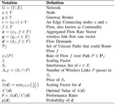
aggregated price for all interference sets. However, in Inequality (20), for each sample demand vector d, the aggregated price of all flows weighted by their demand needs to be larger than the ratio of its probability to its optimal value of λ. DU : minimize X e∈E µe (18) subject to X e∈E AePµe≥µf,∀f ∈F,∀P ∈ P(19)f X f∈F µfdf ≥ p(d) λ∗(d),∀d∈ D (20) where d= (df, f ∈F)
Algorithm II: Mesh Network Routing Under Uncertain Demand
1 ∀e∈E,µe←β
2 xf(P)←0,∀P∈ Pf,∀f∈F
3 loop
4 for∀f∈F do
5 P¯←lowest priced path inPf usingµe
6 µf ←Pe∈EAeP¯µe 7 end for 8 for∀d∈ Ddo 9 µd ←P f∈Fµfdf λ∗(d) p(d) 10 end for 11 µmin←min d∈Dµd
12 dmin←arg mind∈Dµmin
13 ifµmin≥1 14 return 15 for∀f∈F do 16 d′ f ←dminf 17 whiled′ f >0do
18 P ←lowest priced path inPf usingµe
19 δ←min{d′ f,mine∈P A1 eP} 20 d′ f ←d ′ f−δ 21 xf(P)←xf(P) +δ 22 ∀es.t.AeP 6= 0,µe←µe(1 +ǫδAeP ×λ ∗(dmin) p(dmin)) 23 end while 24 end for 25 end loop TABLE III
ROUTINGALGORITHMUNDERUNCERTAINDEMAND
Now we present an approximation algorithm for PU
in Table III. This algorithm (Algorithm II) has the same initialization as the algorithm for problemP(Algorithm
I). Then we march into the iteration, in which we find dmin, the demand whose price µmin is the minimum among others (Lines 4 to 12). If µmin ≥ 1, then the algorithm stops (Lines 13 and 14), since Inequality (8) and (9) would be satisfied for all demand. Otherwise, we will increase the price of dmin by routing more traffic through its node pairs. This procedure (Lines 16 to 22) is the same as what has been described in the lines 4 to 11 of the previous algorithm. Following the same proving sequence for Algorithm I, we are able to prove the similar properties with Algorithm II, which we illustrate the details in the Appendix.
V. SIMULATIONSTUDY
A. Simulation Setup
We evaluate the performance of our algorithms via simulation study. In the simulated wireless mesh net-work, 30 mesh nodes are randomly deployed over a 800×800m2 region, among which 10 nodes are local access points that forward traffic for clients. Node 10 which resides in the center of the deploy region is selected as the gateway router. Each mesh nodes has a transmission range of 250m. The simulated network topology is shown in Fig. 2
0 100 200 300 400 500 600 700 800 0 100 200 300 400 500 600 700 800 Y P osition X Position 0 1 2 3 4 5 6 7 8 9 10 11 12 13 14 15 16 17 18 19 20 21 22 23 24 25 26 27 28 29
Fig. 2. Mesh Network Topology.
B. Traffic Demand Generation
To realistically simulate the traffic demand at each local access point, we analyze the traces collected in the campus wireless LAN network. The network traces used in this work are collected in Spring 2002 at Dartmouth College and provided by CRAWDAD [8].
By analyzing the snmp log trace at each access point, we are able to derive its incoming and outgoing traffic volume in a 5-minute period. We argue that the local access points of a wireless mesh network serve a similar role as the access points of wireless LAN networks at aggregating and forwarding client traffic. Thus, we select
0 0.5 1 1.5 2 2.5 3 3.5 2 4 6 8 10 12 14 16 18 20 Days T
raffic Demand (10Mbits)
0 0.01 0.02 0.03 0.04 0.05 0.06 0.07 0.08 0.09 2 4 6 8 10 12 14 16 18 20 Days T
raffic Demand (10Mbits)
0 0.2 0.4 0.6 0.8 1 1.2 2 4 6 8 10 12 14 16 18 20 Days T
raffic Demand (10Mbits)
0 0.2 0.4 0.6 0.8 1 1.2 1.4 1.6 2 4 6 8 10 12 14 16 18 20 Days T
raffic Demand (10Mbits)
(a) Node 15 (b) Node 16 (c) Node 18 (d) Node 22
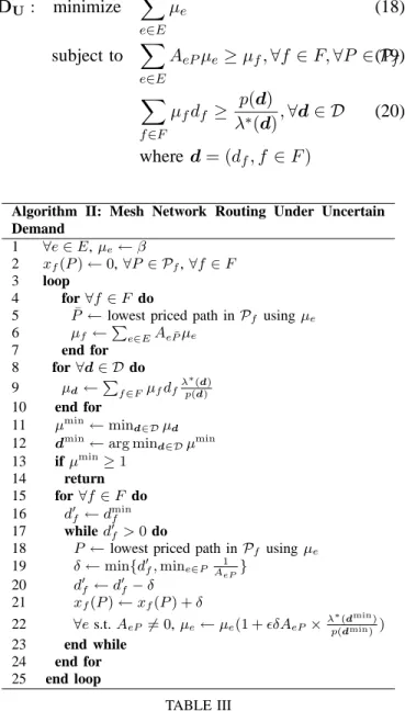
Fig. 3. Traffic Time Series.
10 access points from the Dartmouth campus wireless LAN and assign their traffic traces to the local access points in our simulation. Fig. 3 plots the time series of the traffic volume during one-hour period at the same time of a day (12pm-1pm) from 4 access points for 20 consecutive work days. We remove the weekend days from the traces due to their extreme low traffic volume. From the figure, we observe that the traffic at each access point is highly dynamic and unpredictable due to the insufficient level of aggregation. This observation motivates the need of mesh routing schemes that are aware of the traffic uncertainty.
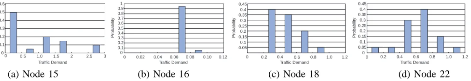
Based on the one-hour traffic volume data from the traces, we further derive the traffic demand distribution for each access point. Essentially, We round the obtained raw traffic volume into finite collection of traffic demand ranges. We treat each piece of traffic volume data as a sample and derive its probability density function. Fig. 4 plots the probability density function for the 4 corresponding access points in Fig. 3.
C. Performance Comparison
We compare the performance of three traffic routing solutions described as follows. In particular, the fist two employ the throughput maximization algorithm under fixed demand (Algorithm I), while the last one employs the algorithm under uncertainty demand (Algorithm II).
• Online Solution: This solution keeps track of the dynamically changing demand and maximizes the throughput based on the current demand of each access point, meanwhile maintaining the fairness among them. Since the access point demand keeps changing, it has to continuously rerun Algorithm I (Table II) to adapt to the new demand. This solution yields the optimal routing result at the cost of frequent routing computation and update.
• Average-Demand-based Solution: This solution es-timates the dynamic traffic demand using the mean value from its probability distribution for each ac-cess point. It computes a fixed route based on this
average demand vector using Algorithm I. Using only the average demand, this solution does not consider the uncertainty of the traffic demand.
• Uncertainty-aware Solution: This solution accom-modates the uncertainty in traffic demand by max-imizing the throughput for all demand vectors nor-malized by their occurring probabilities. In particu-lar, it employs Algorithm II presented in Table III with the traffic distribution derived from the traces.
We evaluate the above three routing solutions under a series of experiments. For each experiment, the traffic demand of each access point is generated based on their probability distribution. We repeat the experiment for 100 times with 100 randomly generated traffic demand vectors. For each experiment, we derive its scaling factor
λ, which is the minimum ratio of throughput and demand among all access points. Fig. 5 plots the sorted values of
λin these100experiments. Evidently, the online solution keeps delivering the optimal scaling factor, at the cost of rerouting for each experiment. Comparatively, average-demand solution provides a single set of routes for all demand vectors, but still achieves a scaling factor no worse than 50% of the optimum, except at the last 5 experiments. Uncertainty-aware solution demonstrate the same trend, but continuously outperforms the average-demand solution by20%. Although there are exceptions in the first 20 experiments when the optimal value of λ
is low, the difference is minor.
After evaluating the overall performance of these so-lutions, we then study them in the granularity of a single experiment. In particular, we are interested to learn the ability of each algorithm at maintaining fairness among different access points. In Fig. 6, we randomly choose one experiment listed in Fig. 5, and plot the scaling factor of aggregated flows achieved on four local access points (node 15, 16, 18, and 22). Here, the average-demand solution achieves the worst fairness among four nodes, as it gives the highest scaling factor for node 18, and
0 0 0.1 0.2 0.3 0.4 0.5 0.6 0.5 1.0 1.5 2 2.5 3 Traffic Demand Probability 0 0 0.1 0.2 0.3 0.4 0.5 0.6 0.7 0.8 0.9 1 0.02 0.04 0.06 0.08 0.10 0.12 Traffic Demand Probability 0 0.05 0.1 0.15 0.2 0.25 0.3 0.35 0.4 0.45 0.2 0.4 0.6 0.8 1.0 1.2 Traffic Demand Probability 0 0 0.05 0.1 0.15 0.2 0.25 0.3 0.35 0.4 0.45 0.2 0.4 0.6 0.8 1.0 1.2 Traffic Demand Probability
(a) Node 15 (b) Node 16 (c) Node 18 (d) Node 22
Fig. 4. Traffic Demand Distribution.
0 0.5 1 1.5 2 2.5 3 3.5 4 4.5 5 0 10 20 30 40 50 60 70 80 90 100 λ Experiment Average Uncertain Online
Fig. 5. Comparison of Three Algorithms
the lowest for 221. On the other hand, online algorithm maintains the best fairness among four nodes, since its result is tuned on-the-fly to the specific demand. Finally, the uncertainty-aware solution trades off well between the former two, by returning the scaling factor which is much higher than average-demand solution (observing node 22), yet only slightly lower than the online solution (observing node 15 and 18).
0 0.5 1 1.5 2 2.5 3 Node 15 Average Uncertain Online
Node 16 Node 18 Node 22
λ
Fig. 6. Comparison of Aggregated Flows from Different Access
Points
In Fig. 7, we compare the aggregated throughput of all local access points enabled by these three solutions. Obviously, throughout all experiments, the aggregated
1Recall in Fig. 5, the scaling factor achieved at each experiment
is the lowest value among all access nodes.
throughput remains the same for average-demand and uncertainty-aware solutions since they stick to only one set of routes. The latter solution outperforms the former one, as confirmed by our observation in Fig. 5 in terms of scaling factor. The online solution, however, results in unstable aggregate throughput over different experiments. While its maximum value is higher than the other two solutions, the minimum throughput is also well below both of them.
0 1 2 3 4 5 6 Min Max Average Uncertain Online Throughput
Fig. 7. Comparison of Aggregated Throughput
In summary, our simulation results demonstrate that our statistical problem formulation could effectively in-corporate the traffic demand uncertainty in routing op-timization, and its algorithm outperforms the algorithm which only considers the static traffic demand.
VI. RELATEDWORK
We evaluate and highlight our original contributions in light of previous related work.
The problem of wireless mesh network routing has been extensively studied in the existing literature. For example, routing algorithms are proposed to improve the throughput for wireless mesh networks via integrating MAC layer information [15], such as expected packet transmission time [4]. Joint solutions for channel alloca-tion and routing are explored in [5] using a centralized algorithm and in [3] in a distributed fashion. These heuristic solutions lack the theoretical foundation to analyze how well the network performs globally (e.g.,
whether the network resource is fully utilized, whether the flows share the network in a fair fashion) under their routing schemes. There are also theoretical studies that formulate these network planning decisions into optimization problems. For example, the work of [6] studies the optimal solution of joint channel assignment and routing for maximum throughput under a multi-commodity flow problem formulation and solves it via linear programming. The work of [16] presents band-width allocation schemes to achieve maximum through-put and lexicographical max-min fairness respectively. [17] presents a rate limiting scheme to enforce the fairness among different local access points. These re-sults provide valuable analytical insights to the mesh network design under ideal assumptions such as known static traffic input. It is not clear whether they will be unsuitable for practical use under highly dynamic traffic situation. Different from these existing works, our work explicitly incorporates traffic uncertainty into the routing optimization, thus better fits the routing need in the dynamic wireless mesh networks.
Trace analysis has been used to study the behavior of wireless networks in many recent works. To name a few, the works of [18], [19] analyze a campus-wide wireless network traffic and its changes in two years. [20] statisti-cally characterizes both static flows and roaming flows in a large campus wireless network. In [21], the flow level traffic pattern is used to design a scheduling algorithm for end-host multi-homing. Different from these existing works, which focus on either user behavior, network flow or link performances, we provide a framework that integrates traffic uncertainty model with its performance optimization.
Our work is also related to dynamic traffic engineer-ing [22] in Internet and oblivious routengineer-ing [23], which also consider the impact of demand uncertainty in make routing decisions. The major difference between our work and these existing works lies in the different net-work models of wireless mesh netnet-work and Internet and the different problem formulations. In particular, traffic engineering tries to minimize the congestion (utilization) of the wired links of a network. In multihop wireless network, wireless link utilization can not be used to characterize the network performance due to the location dependent contention in the vicinity area. The objective of our research is to maximize the ratio between flow throughput and its demand, subject to the schedulability and fairness constraints.
VII. CONCLUSION
This paper studies the throughput optimization routing problem for wireless mesh networks. Different from ex-isting works which assume fixed traffic demand known a priori, this work considers the traffic demand uncertainty. It models such uncertain demand with random variables, extends the classical maximum concurrent flow problem with statistical demand input, and derives approximation algorithms for uncertainty-aware traffic routing. Simu-lation study is conducted based on the traffic demands from the real wireless network traces. The results show that our problem formulation and algorithm could effec-tively incorporate the traffic demand uncertainty.
REFERENCES
[1] “Seattle wireless,” http://www.seattlewireless.net. [2] “Mit roofnet,” http://www.pdos.lcs.mit.edu/roofnet/.
[3] A. Raniwala and T. Chiueh, “Architecture and algorithms for an ieee 802.11-based multi-channel wireless mesh network,” in Proc. of IEEE INFOCOM, 2005.
[4] Richard Draves, Jitendra Padhye, and Brian Zill, “Routing in multi-radio, multi-hop wireless mesh networks,” in Proc. of ACM Mobicom, 2004, pp. 114–128.
[5] A. Raniwala, K. Gopalan, and T. Chiueh, “Centralized channel assignment and routing algorithms for multi-channel wireless
mesh networks,” Mobile Computing and Communications
Review, vol. 8, no. 2, pp. 50–65, 2004.
[6] Mansoor Alicherry, Randeep Bhatia, and Li Li, “Joint channel assignment and routing for throughput optimization in multi-radio wireless mesh networks,” in Proc. of ACM MobiCom, 2005.
[7] Murali Kodialam and Thyaga Nandagopal, “Characterizing
the capacity region in multi-radio multi-channel wireless mesh networks,” in Proc. of IEEE WiMesh, 2005.
[8] “A community resource for archiving wireless data at dart-mouth,” http://crawdad.cs.dartmouth.edu/.
[9] P. Gupta and P.R. Kumar, “The capacity of wireless networks,” IEEE Trans. on Information Theory, pp. 388–404, 2000. [10] K. Jain, J. Padhye, V. Padmanabhan, and L. Qiu, “Impact on
interference on multi-hop wireless network performance,” in Proc. of Mobicom, September 2003.
[11] V. S. Anil Kumar, M. V. Marathe, S. Parthasarathy, and A. Srini-vasan, “Algorithmic aspects of capacity in wireless networks,” in Proc. of ACM SIGMETRICS, 2005, pp. 133–144.
[12] Yuan Xue, Baochun Li, and Klara Nahrstedt, “Optimal
re-source allocation in wireless ad hoc networks: A price-based approach,” IEEE Transactions on Mobile Computing, vol. 5, no. 4, pp. 347–364, April 2006.
[13] “Ilog cplex mathematical programming optimizers,”
http://www.ilog.com/products/cplex.
[14] N. Garg and J. Konemann, “Faster and simpler algorithms for multicommodity flow and other fractional packing problems,” in Proc. of IEEE FOCS, 1998.
[15] Sanjit Biswas and Robert Morris, “Exor: opportunistic
multi-hop routing for wireless networks,” in Proc. of ACM
SIG-COMM, 2005, pp. 133–144.
[16] J. Tang, G. Xue, and W. Zhang, “Maximum throughput and fair bandwidth allocation in multi-channel wireless mesh networks,” in Proc. of IEEE INFOCOM, 2006.
[17] Violeta Gambiroza, Bahareh Sadeghi, and Edward W. Knightly, “End-to-end performance and fairness in multihop wireless backhaul networks,” in Proc. of ACM MobiCom, 2004. [18] David Kotz and Kobby Essien, “Analysis of a campus-wide
wireless network,” in ACM MobiCom, 2002, pp. 107–118. [19] Tristan Henderson, David Kotz, and Ilya Abyzov, “The
chang-ing usage of a mature campus-wide wireless network,” in Proc. of ACM MobiCom, 2004, pp. 187–201.
[20] Xiaoqiao (George) Meng, Starsky H. Y. Wong, Yuan Yuan, and Songwu Lu, “Characterizing flows in large wireless data networks,” in Proc. of ACM MobiCom, 2004.
[21] Nathanael Thompson, Guanghui He, and Haiyun Luo, “Flow scheduling for end-host multihoming,” in Proceedings of IEEE INFOCOM, 2006.
[22] Hao Wang, Haiyong Xie, Lili Qiu, Yang Richard Yang, Yin Zhang, and Albert Greenberg, “Cope: traffic engineering in dynamic networks,” in Proc. of ACM SIGCOMM, 2006. [23] Yossi Azar, Edith Cohen, Amos Fiat, Haim Kaplan, and Harald
Racke, “Optimal oblivious routing in polynomial time,” J.
Comput. Syst. Sci., vol. 69, no. 3, 2004.
VIII. APPENDIX
We show the proofs to the lemmas and theorem in the paper. Here, f∗ is the result returned by the algorithm.
OP T is the optimal value of D as well as P. A. Proof for Lemma 1
Proof: We first make the following denotations. Regarding a set of price assignmentsµe forSe (e∈E),
the objective function of D is Lµe , P
e∈Ec·µe. Let Pµe(f)be the minimum path of the flowf ∈F usingµ
e. µ(Pµe(f)),P
e∈EAePµe(f)µe is the aggregated price
of Pµe(f). Each phase contains |F| iterations, where
traffic for each flow in F is routed according to its demand. In each iteration, the price of an interference set is updated. We use µ(ei)(j) to denote the price of Se for e∈E after thejth iteration of theith phase. Regarding
µ(ei)(j), we simplify the notation Lµ (i)(j) e into L(i)(j), Pµ(i)(j) e intoP(i)(j), andµ(Pµ (i)(j) e )intoµ(P(i)(j)). Based
on the price update function (Line 11 in Tab. II), we have
L(i)(j) = X e∈E µ(ei)(j−1)+ǫ X e∈P(i)(j−1) AeP(i)(j−1)µe(i)(j−1)d(fj) = L(i)(j−1)+d(fj)µ(P(i)(j−1))
The price assignment at the start of the (i+ 1)th phase are the same as that at the end of the ith phase, i.e.,
µ(ei+1)(0) = µ(ei)(|F|). The price of any interference set Se is initialized as µ(1)(0)e =µe(0)(|F|) =β/c. Hence, L(i)(|F|)≤L(i)(0)+ǫ |F| X j=1 d(fj)µ(P(i)(|F|))
since the edge lengths are monotonically increasing.
Let us defineµ(i)(|F|) =P|jF=1| d(fj)µ(P(i)(|F|)). Then
the objective ofDis to minimizeL(i)(|F|), subject to the constraint thatµ(i)(|F|)≥1. This constraint can be easily satisfied if we scale the length of all inference sets by 1/µ(i)(|F|). So D is equivalent to finding a set of infer-ence set lengths, such that Lµ((ii)()(||FF||)) is minimized. Thus
the optimal value ofD is OP T ,minµ(i)(|F|) L (i)(|F|) µ(i)(|F|). Since Lµ((ii)()(||FF||)) ≥OP T, we have L(i)(|F|)≤ β|E| 1−ǫe ǫ(i−1) OP T(1−ǫ) Since L(0)(|F|)=β|E|, we have L(i)(|F|) ≤ β|E| (1−ǫ/OP T)i = β|E| (1−ǫ/OP T)(1 + ǫ OP T −ǫ) i−1 ≤ β|E| (1−ǫ/OP T)e ǫ(i−1) OP T−ǫ ≤ β|E| 1−ǫe ǫ(i−1) OP T(1−ǫ)
where the last inequality assumes thatOP T ≥1. The algorithm stops at the first phasetfor whichL(t)(|F|)≥
1. Therefore, 1≤L(t)(|F|) ≤ β|E| 1−ǫe ǫ(t−1) OP T(1−ǫ) which implies OP T t−1 ≤ ǫ (1−ǫ) lnβ1|−Eǫ| (21) Now consider an interference setSe. For everycunits
of flow routed through Se, we increase its price by at
least a factor(1 +ǫ). Initially, its length isβ/c and after
t−1 phases, sinceL(t)(|F|)<1, the price of Se satisfies µ(et−1)(|F|) < 1/c. Therefore the total amount of flow
through Se in the first t−1 phases is strictly less than
log1+ǫ 1β/c/c = log1+ǫ1/β times its capacity. Thus, scaling the flow by log1+ǫ1/β will yield a feasible solution. Since in each phase, d(f) units of data are routed for each flow, we have f∗= logt−1
1+ǫ1/β.
B. Proof for Lemma 2
Proof: By Lemma 1, scaling the final flow by log1+ǫ1/β yields a feasible solution. Therefore,
OP T
Substituting the bound on OP T /(t − 1) from In Equality (21), we get OP T f∗ < ǫlog1+ǫ1/β (1−ǫ) lnβ1−|Eǫ| = ǫ (1−ǫ) ln(1 +ǫ) ln 1/β lnβ1−|Eǫ| When β = (|E|/(1−ǫ))−1/ǫ, the above in Equality becomes OP T f∗ < ǫ (1−ǫ)2ln(1 +ǫ) ≤ ǫ (1−ǫ)2(ǫ−ǫ2/2) 1 ≤(1−ǫ)3 ≤ (1−3ǫ)
C. Proof for Lemma 3
Proof: From In Equality (22) and weak-duality, we have
1≤ OP T
f∗ <log1+ǫ1/β
Hence, the number of phases t is strictly less than 1 + OP Tlog1+ǫ1/β. If β = (|E|/(1 −ǫ))−1/ǫ, then t≤1 +OP Tǫ log1+ǫ1|E−|ǫ
These lemmas require that OP T ≥ 1. The running time of the algorithm also depends on OP T. Thus we need to ensure that OP T is at least one and not too large. Let ζi be the maximum traffic value of flow fi
when all other flows have zero traffic. Letζ = mini d(ζfii).
Since at best all single commodity maximum flows can be routed simultaneously,ζ is an upper bound onf∗. On the other hand, routing 1/|F| fraction of each flow of value ζi is a feasible solution, which implies that ζ/|F|
is a lower bound on OP T. To ensure that OP T ≥ 1, we can scale the original demands so that ζ/|F| is at least one. However, by doing so, OP T might be made as large as |F|, which is also undesirable.
To reduce the dependence on the number of phases on OP T, we adopt the following technique. If the algorithm does not stop after T = 2ǫlog1+ǫ 1|E−|ǫ phases, it means that OP T >2. We then double demands of all commodities, so that OP T is halved and still at least 1. We then continue the algorithm, and double demands again if it does not stop after T phases.
D. Proof for Lemma 4
Proof: The above demand-doubling procedure is repeated for at mostlog|F|times. Thus, the total number of phases is at most Tlogk. Since each phase contains
k iterations, the algorithm runs for at most kTlogk
iterations.
Now we observe how many steps are within each iteration. For each step except for the last step in an iteration, the algorithm increases the length of some edge (the bottleneck edge on t) by 1 +ǫ. de has initial value
β/ce and value at most 1/ce before the final step of the
algorithm. Otherwise, the stop criterion of the algorithm,
P
e∈Ece·de≥1, would have been reached. This means
that the length of an edge can be updated in at most log1+ǫ 1β = 1ǫlog1+ǫ1|E−|ǫ steps. Therefore, the algorithm contains at most |E| ǫ log1+ǫ1|E−|ǫ ≤ |E| ǫ2 log |E|
1−ǫ such “normal” steps, and kTlogk ≤ 2klogǫ2 klog
|E|
1−ǫ “final” steps. Each step
con-tains a minimum overlay spanning tree operation. E. Proof for Theorem 1
Proof: Computing ζi corresponds to the maximum
flow problem, where fi is the only commodity. The
running time of gettingζi isO(|ǫE2|(logU))·Tmp, where U is the length of the longest unicast route, and Tmp
denotes the running time to find the minimum path. Such an operation has to be repeated for each flow. Also from the result of Lemma 4, we can obtain the total running time as described by the theorem.
F. Proof for Algorithm under Uncertain Demand The proof for the algorithm under uncertain demand follows the same sequence as the proof for the algorithm under fixed demand, with minor modification. We start with Lemma 1. Each phase of the algorithm contains |F|iterations, where traffic for each flow in F is routed according to its demand. We reuse the same denotations defined in the original proof to Lemma 1. We further introduce d(i) as the demand vector chosen at the ith phase.
Based on the price update function (Line 11 in Tab. II), we have
L(i)(j)
= L(i)(j−1)+d(fj)µ(P(i)(j−1))
λ∗(d(i))
p(d(i)) The price assignment at the start of the (i+ 1)th phase are the same as that at the end of the ith phase, i.e.,
µ(ei+1)(0) = µ(ei)(|F|). The price of any interference set Se is initialized as µ(1)(0)e =µe(0)(|F|)=β/c. Hence, L(i)(|F|) = L(i)(0)+ǫ |F| X j=1 d(fj)µ(P(i)(j−1)) λ∗(d(i)) p(d(i)) ≤ L(i)(0)+ǫ |F| X j=1 d(fj)µ(P(i)(|F|)) λ∗(d(i)) p(d(i))
since the edge lengths are monotonically increasing.
Let us define µ(i)(|F|) =
P|F|
j=1d(fj)µ(P(i)(|F|))λ
∗(d(i))
p(d(i)) . Then the objective
of D is to minimize L(i)(|F|), subject to the constraint that µ(i)(|F|)≥1, i.e., Lµ((ii)()(||FF||)) ≥OP T.
The rest of the proof follows the same as the original proof to Lemma 1. The proofs to Lemma 2, 3, 4, and