SRAD: Smart Routing Algorithm Design for
Supporting IoT Network Architecture
Annop Monsakul
Faculty of Information Technology, Thai-Nichi Institute of Technology, Bangkok, Thailand
Abstract: The smart things require applications and services such as speed wireless, definition IP video cameras, and high-bandwidth connectivity. Therefore, Fog computing is responsible reducing the amount of data sent to the cloud with smart router over the core network. The IP/MPLS network design to support unicast traffic under delay constraints is a severe problem. To realize such design, especially for communication networks that can be represented by M/M/1 model, this paper develops an algorithm based on Mesh Network Topological Optimization and Routing (MENTOR)-II was called “Smart MENTOR-II”. The simulation results show that, in almost all test cases, the proposed algorithm yields lower installation cost and delay constraints than the ordinary MENTOR-II.
Keywords: Smart Things, Fog Computing, Cloud Computing, IP/MPLS Network Design, MENTOR-II Algorithm, M/M/1 Model, Unicast Traffic.
1.
Introduction
Nowadays, Internet of Things (IoT) has been enjoying a very rapid growth. In 2020, the evolution of so-called smart things around 50 billion connected devices, which include machines, wearables, sensors and embedded systems. The device connected to WiFi, Bluetooth, ZigBee, UWB, 4G/LTE, NFC, LoRa, Sigfox, and WiMax. The IoT systems use of Internet protocols to run over IP rather than proprietary transports. Also greater adoption and support for IPv4/IPv6 in carrier networks. The smart devices are a part of the broader concept such as agriculture, smart city, industrial automation, smart home, smart grid, healthcare, intelligent buildings, intelligent transportation, and defense. The device is using all IP address based, IP/MPLS [1] is used for the backhaul and core transport networks that connect various end-points. Also, although the current approach toward IoT is being based on centralized management of IoT using cluster of cloud-based servers, it is being recognized that with the fast increase in the number of objects connected to the IoT, the centralized cloud-based management [15]. Fog computing [2] adds a hierarchy approach to computing, storage, control and networking anywhere along the continuum from the cloud to smart things [16], to meet these challenges in high performance and interoperable way. Therefore, a routing algorithm finds the best path on IP/MPLS core network is designed to give effect to service delivery, and service support is significant.
Internet Protocol (IP) network design which concerns unicast routing [3] remains a severe problem. The problem is even more challenging if we choose to manage the traffic by the appropriate setting of link weights in the Open Shortest Path First (OSPF) protocol instead of using the overlay network technique. This kind of problem can be classified as Mixed Integer Linear Programming (MIP) [4].
To reduce the complexity of the network design process, Kershenbaum et al. [5] developed a heuristic algorithm, called MENTOR (Mesh Network Topological Optimization and Routing). The networks designed by this algorithm may be able to give near-optimal routing performance [6]. MENTOR can also be used to design virtual circuit switching and packet switching networks such as Asynchronous Transfer Mode (ATM) and frame relay. However, it cannot be directly used to design routers or Multiprotocol Label Switching (MPLS) networks [7] that employ OSPF or Intermediate-System-to-Intermediate-System (ISIS) routing protocol. This is because MENTOR does not perform an appropriate link weight setting. Cahn [8] improved the MENTOR algorithm such that appropriate OSPF link weights can be set during the design process using Incremental Shortest Path (ISP). This improved version is known as MENTOR-II. We use to design for minimum distance networks has increased complexity. However, it should be noted that almost all the above design algorithms were being developed for networks with only unicast traffic. To efficiently design communication networks with delay constraints, especially the networks that can be represented by M/M/1 model [9], this paper develops an algorithm based on MENTOR-II. Instead of fixing all design parameters as in the ordinary MENTOR-II, this algorithm determines the maximum utilization of a link based on its delay and capacity. It allows us to control directly of the network delay. Here, the performances of networks designed by the proposed algorithm are evaluated regarding installation cost and compared with those of networks designed by the ordinary MENTOR-II for various traffic demands and different numbers of nodes.
The rest of the paper is organized as follows. In Section II, the MENTOR and MENTOR-II algorithms are introduced. In Section III, we explain how the maximum link utilization is determined by the link delay and capacity. In Section IV, an example of 10-node network design is given. In Section V, given a maximum network delay of 5 ms and maximum link delays of 1.712 ms, 3 ms, and 5 ms for 10-node networks, respectively, the cost of networks designed by the proposed algorithm is evaluated and compared with that of networks designed by the MENTOR-II algorithm.
2.
Background
2.1 IoT Network Architecture Layers
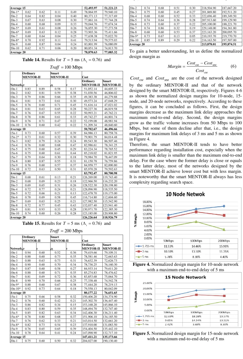
Layer 2: Multi-Service Edge Layer 3: Core Network Layer 4: Data Center Cloud
Layer 1: Embedded Systems and Sensors
Figure 1. The 4 Layers of IoT Network Architecture
1) Embedded Systems and Sensors Layers: the first layer of the IoT architecture is comprised of embedded systems and sensors [17]. As such, these are smart, less smart things, vehicles, and machines. The device connected to wired or wireless technology. Also, although the current approach toward smart things is based on rich (mobile) clients, edge stack, routing, QoS, and CAC.
2) Multi-Service Edge:The variance of smart devices and their potentially enormous numbers highlight the importance of the multi-service edge in the IoT architecture. This layer must support many different protocols, such as Bluetooth, Zigbee, WiFi, 3G, 4G, Ethernet, and PLC to accommodate a variety of smart device. Therefore, the only way to communicate between Edge Router, Access Point, Fog Computing, Storage, Data Management, Control Logic, and Industrial Ethernet.
3) Core Network Layer: The architecture of the core network layer is IP/MPLS architecture. The function of this layer is to provide paths to carry and exchange data and network information between multiple sub-networks as require Low Jitter, Precise Scheduling, Loss-less Convergence, Multi-path switching.In this layer responsible, there are QoS, Multicast, Security, Network Service and Mobile Packet Core. Such as Mobility and Infrastructure Routing, Distributed Data Center, and Fog Service Delivery Support.
4) Data Center Cloud Layer: The architecture of the data center cloud layer is that ensure efficiency agility and openness for your users, applications, and data. Again, cloud services in this layer are Data Center Computer, Storage, Networking, Cloud Computing, Service/Apps Delivery Support, and Cisco’s Apps.
2.2 MENTOR Algorithm
MENTOR is our archetype for a high-quality, low-complexity of core network design s a heuristic algorithm. The total complexity of an intelligent algorithm is onlyO n( 2). The properties of networks designed by this algorithm are: 1) traffic is routed on relatively direct paths, 2) links have reasonable utilization, and 3) relatively high-capacity links are used.
MENTOR starts with clustering process. In this stage, network nodes are classified into end nodes and core nodes using a clustering algorithm. Examples of possible clustering algorithms are threshold clustering and K-mean clustering. Here, we consider only the case where traffic demands are distributed equivalently among all nodes. All the nodes can be considered as core nodes.
Next, a suitable tree is formed to interconnect all (core) nodes. Kershenbaum et al. [11] suggested a heuristic algorithm, which can be thought of as a modification of Prim’s algorithm and Dijkstra’s algorithm to build the tree. This algorithm works similarly to Dijkstra’s algorithm but with a tunable parameter (0≤ ≤ 1). Note that = 0 and 1 correspond to Minimum Spanning Tree (MST) and Shortest Path Tree (SPT), respectively.
Given a tree, the objective of MENTOR is to add a direct link between each pair of nodes if the amount of traffic is reasonable. Let be the maximum link utilization, and hence the minimum link utilization can be defined as (1s) where 0 ≤ s ≤ 1 is the slack. Consider a pair of nodes, namely
A and B. Let CAB and lAB be the link capacity and
accumulated load flow between nodes A and B, respectively. If traffic between nodes A and B is too small, i.e., lAB <
(1s) CAB, no link is added, and all traffic lAB is
overflowed to the next most direct path. A link is added if traffic is in between the minimum and maximum link utilization, i.e., (1s) CAB≤ lAB ≤ CAB. However, if lAB >
CAB, a direct link is added only when traffic bifurcation
among multiple routes is possible. That is, a new link of CAB
is added to serve a portion of traffic CAB, and the left
portion lAB CAB is overflowed to the next most direct
path. Otherwise, no link is added, and all traffic lAB is
overflowed to the next most direct path. 2.3 MENTOR-II Algorithm
It has to do considerably more work at the direct-link addition stage. Similar to the previous algorithm, MENTOR-II [12] starts with clustering network nodes and building a good spanning tree between core nodes. However, when considering adding a direct link to serve the traffic demand between a pair of nodes, MENTOR-II calculates an appropriate weight for this link by using Incremental Shortest Path (ISP) algorithm. The concept of MENTOR-II can be described as follows:
1) Set the weight for each link in the selected good spanning tree proportional to the installation cost of the link;
2) Let dspt(A, B) be the shortest path distance between
nodes A and B through the spanning tree, and consider adding a direct link between each pair of nodes in decreasing order of dspt(∙);
3) When considering whether to add a link LAB between
A and B, the weight wAB of the LAB is initially set to a
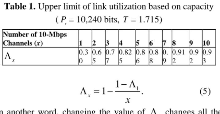
Number of 10-Mbps
Channels (x) 1 2 3 4 5 6 7 8 9 10
x
0.30 0.6 5
0.7 7
0.82 5 0.86
0.8 8
0. 9
0.91 2
0.9 2
0.9 3 through LAB as much as possible by lowering wAB. The
constraint is that wAB should be greater or equal to the
installation cost;
4)
The LAB is added if an eligible value of wAB can befound and the amount of traffic flow though it falls in the reasonable zone defined by , CAB, and
s
.When all possible direct links are considered, they are assigned with appropriate weights which ensure the shortest path routing.
3.
Design parameters
The MENTOR family allows us to construct good mesh networks efficiently. However, it does not give any idea of how to choose the design parameters, e.g., , , and s, to achieve the designed constraints. Hence, one may have to perform an exhaustive search of all possible combination of such parameters to find the optimum solution.
In this paper, focus on the problem of minimizing the installation cost with delay constraints such as the maximum link delay and maximum end-to-end delay, especially for networks that can be represented by M/M/1 model [13]. For this model, the average link delay is given by
T
T
p
T
q p
T
is the propagation delay which depends on the linkdistance, and
T
q is the average queuing delay:
1
s q
P
T
C
U
s
P
is the average packet size in a bit, Uis the link utilization, and Cis the link capacity, i.e., for a network designed by MENTOR,
1
.
s q
P
T
C
It should be noted that, for the ordinary MENTOR, the design parameters such as and
P
s are kept constant for all links. As a consequence, a link with small capacity always suffers more delay than the one with large capacity. To avoid the significant delay of the former link, one should try to keep as small as possible. An algorithm may lead to inefficient utilization of a large-capacity link, which is more expensive. Therefore, from (1) and (3), instead of using the same value of for all links, let be determined by
: 1
P
sT C
TIt is the maximum allowable link delay of the overall network. Based on (4), a link with a large capacity is allowed to have more efficient utilization for given average packet size and maximum allowable link delay, e.g., see Table I. Another advantage of using the variable maximum link utilization of (4) is that the MENTOR search domain can be reduced. Let Cx x Cg where 1 C1 is the capacity of a single-channel link, e.g., 10 Mbps in Table 1. From (4), the upper limit
x of
x for a link of capacityC
xTable 1.Upper limit of link utilization based on capacity (Ps= 10,240 bits, T= 1.715)
1
1
1.
x
x
In another word, changing the value of
1 changes all the values of other
x.
As a result, in the search process, only1
is subjected to be varied to find the optimum solution. In comparison with the ordinary MENTOR-II, the optimum search domain of the maximum link utilization is reduced from all possible
in (0,1) to (0,
1).4.
Experimental Setup
4.1 Requirements
Let us assume that an organization designs a network composed of 10 core nodes as shown in Figure 2, where the distance between any pair of them is within 100 km. Moreover, this network must support unicast traffic. Table 2 shows the unicast traffic demands between core nodes in the network.
Assume further that one or more 10-Mbps channels can be installed in a link. Table 3 shows the installation cost of 10-Mbps channel links between all possible node pairs. Let
P
sbe 12,288 bits. The goal of the network design is to find the network with minimum installation cost, given that the maximum end-to-end delay and maximum link delay are 5 ms and 1.715 ms, respectively.
Table 2. Unicast traffic demands between backbone nodes S\D N1 N2 N3 N4 N5 N6 N7 N8 N9 N10 N1 0 9512 3130 3516 3734 3620 14938 3564 4618 3366
N2 9512 0 4576 3696 3972 5060 6932 4266 6758 5222
N3 3130 4576 0 3834 4466 4448 3182 4824 3970 17572
N4 3516 3696 3834 0 14766 4202 4374 8208 3842 3562
N5 3734 3972 4466 14766 0 3982 4510 6738 3712 4122
N6 3620 5060 4448 4202 3982 0 3866 8042 12420 4360
N7 14938 6932 3182 4374 4510 3866 0 4128 4742 3322
N8 3564 4266 4824 8208 6738 8042 4128 0 5846 4386
N9 4618 6758 3970 3842 3712 12420 4742 5846 0 4092
N10 3366 5222 17572 3562 4122 4360 3322 4386 4092 0 Unit: kbps Table 3. Installation cost of 10-Mbps channel links S\D N1 N2 N3 N4 N5 N6 N7 N8 N9 N10 N1 1896 2224 2282 2118 3180 1238 2674 3994 2176
N2 1896 1638 2272 2086 2422 2588 2358 2902 1520
N3 2224 1638 958 832 1168 2230 922 1988 320
N4 2282 2272 958 396 1392 1900 678 2340 1062
N5 2118 2086 832 396 1434 1814 778 2372 924
N6 3180 2422 1168 1392 1434 3044 934 1150 1240
N7 1238 2588 2230 1900 1814 3044 2374 3968 2242
N8 2674 2358 922 678 778 934 2374 1882 1040
N9 3994 2902 1988 2340 2372 1150 3968 1882 2022
N10 2176 1520 320 1062 924 1240 2242 1040 2022
4.2 Results
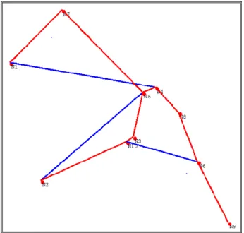
consists of 9 branches: (1,7), (5,7), (3,5), (3,10), (2,10), (4,5), (4,8), (6,8), and (6,9).
4.3 Ordinary MENTOR-II
The ordinary MENTOR-II algorithm runs for all possible values of and s to find a combination that gives the least installation cost while the network delay and link delay are within desired ranges. Since both and s are real numbers that range between 0 and 1, it is not possible to perform an exhaustive search for all possible combinations of them. However, the suboptimum search can be performed as follows. First, and s is initialized to 0.01. Then, they are increased by 0.01 at a time till the maximum value which is set to 0.99.
Figure 2 is shown the resulting network with = 0.73 and
s = 0.93. It achieves a minimum cost of 36,027.29. The network has 12 links of which utilization, load, and capacity are shown in Table 4.
Figure 2. Network designed by the ordinary MENTOR-II
Table 4. Utilization, load, and capacity of the installed links [x,y] U[x,y] load[x,y] C[x,y] [x,y] U[x,y] load[x,y] C[x,y]
[1,4] 0.69 35,188 51,200 [4,5] 0.69 91,258 133,120 [4,1] 0.70 36,084 51,200 [5,4] 0.69 91,258 133,120 [1,7] 0.49 15,066 30,720 [4,8] 0.68 69,594 102,400 [7,1] 0.49 15,066 30,720 [8,4] 0.67 69,082 102,400 [2,5] 0.70 28,506 40,960 [5,7] 0.70 36,080 51,200 [5,2] 0.71 29,018 40,960 [7,5] 0.69 35,184 51,200 [2,10] 0.71 21,744 30,720 [6,8] 0.65 46,728 71,680 [10,2] 0.72 22,128 30,720 [8,6] 0.66 47,112 71,680 [3,5] 0.63 38,450 61,440 [6,9] 0.71 51,152 71,680 [5,3] 0.63 38,834 61,440 [9,6] 0.70 50,128 71,680 [3,10] 0.70 50,092 71,680 [6,10] 0.71 28,944 40,960 [10,3] 0.70 49,836 71,680 [10,6] 0.71 29,072 40,960
4.4 Smart MENTOR-II
The design procedure of the proposed algorithm is somewhat similar to that of the ordinary MENTOR-II except that the search domain of maximum link utilization is limited to all possible values in(0,
1). Since the required link delay T is 1.715, we have
1= 0.3 from (3). An algorithm means the computational complexity of the smart MENTOR-II is about one-third of that of the ordinary one.The figure 3 is shown the resulting network with
1= 0.28 ands
= 0.40. It achieves a minimum cost of 30,368.98. The maximum link utilization for various capacities is listed in Table 5. The network has 20 links of which utilization, load, and capacity as shown in Table 6.Table 5. Maximum link utilization based on capacity Number of 10-Mbps
Channels (x) 1 2 3 4 5 6 7 8 9 10
x
0.28 0.64 0.76 0.82 0.86 0.88 0.90 0.91 0.92 0.93Table 6. Utilization, load, and capacity of the installed links [x,y] U[x,y] load[x,y] C[x,y] [x,y] U[x,y] load[x,y] C[x,y] [1,2] 0.65 20,066 30,720 [4,8] 0.72 29,510 40,960
[2,1] 0.65 20,066 30,720 [8,4] 0.72 29,510 40,960
[1,5] 0.46 14,072 30,720 [4,10] 0.53 16,388 30,720
[5,1] 0.47 14,456 30,720 [10,4] 0.53 16,260 30,720
[1,6] 0.41 8,366 20,480 [5,7] 0.56 11,398 20,480
[6,1] 0.41 8,494 20,480 [7,5] 0.54 11,142 20,480
[1,7] 0.72 22,126 30,720 [5,8] 0.77 31,622 40,960
[7,1] 0.72 21,998 30,720 [8,5] 0.77 31,622 40,960
[2,8] 0.46 9,454 20,480 [5,10] 0.57 11,672 20,480
[8,2] 0.47 9,582 20,480 [10,5] 0.57 11,672 20,480
[2,10] 0.68 27,846 40,960 [6,7] 0.43 8,864 20,480
[10,2] 0.69 28,230 40,960 [7,6] 0.43 8,736 20,480
[3,5] 0.68 27,982 40,960 [6,8] 0.74 30,222 40,960
[5,3] 0.70 28,750 40,960 [8,6] 0.75 30,862 40,960
[3,10] 0.73 22,276 30,720 [6,9] 0.72 22,164 30,720
[10,3] 0.73 22,404 30,720 [9,6] 0.71 21,908 30,720
[4,5] 0.72 22,244 30,720 [8,9] 0.58 17,882 30,720
[5,4] 0.73 22,500 30,720 [9,8] 0.57 17,498 30,720
[4,7] 0.43 8,758 20,480 [9,10] 0.54 10,978 20,480
[7,4] 0.42 8,630 20,480 [10,9] 0.54 11,106 20,480
Figure 3. Network designed by the smart MENTOR-II
5.
Performance evaluation
5.1 Setup
For all node distributions, the maximum node distance is limited to 100 km. The unicast traffic demands for each requirement set are also generated by DELITE with the following assumptions:
1) All nodes have the same total amount of unicast traffic in and unicast traffic out, denoted by Traff
;
2) The unicast traffic between any pair of nodes is inversely proportional to the distance between them.
The effect of the amount of traffic on the design performance, traffic demand matrices as of 50 Mbps, 100 Mbps, and 200 Mbps are generated for each node distribution. Let for the network traffic including unicast be 10,240 bits.
Assume that one or more 10-Mbps channels can be installed in a link, and for each channel, the fixed installation cost is 250 unit and the variable installation cost is 2 unit per km. For each requirement set, the suboptimum search described in the previous section is performed to find the minimum cost for a maximum end-to-end delay of 5 ms and maximum link delays of 1.715 ms, 3 ms, and 5 ms, i.e.,
1= 0.3, 0.6, 0.76, respectively.5.2 Results
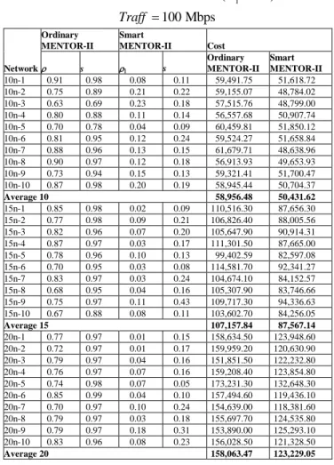
The tables 7-15 present the results obtained by the ordinary MENTOR-II and the modified one for nine combinations of three different traffic volumes, i.e., Traff = 50 Mbps, 100 Mbps, 200 Mbps, and three different link delay requirements, i.e., 1.71 ms, 3 ms, and 5 ms.
Table 7. Results for T 1.715 ms ( 1 0.3) and
50 Mbps Traff
Network Ordinary MENTOR-II
Smart
MENTOR-II Cost
s s
Ordinary MENTOR-II
Smart MENTOR-II
10n-1 0.73 0.94 0.12 0.30 34,887.19 31,446.08 10n-2 0.73 0.93 0.15 0.29 36,027.29 30,368.98 10n-3 0.81 0.97 0.21 0.37 32,627.71 30,296.31 10n-4 0.81 0.94 0.18 0.27 33,198.99 30,686.68 10n-5 0.70 0.84 0.06 0.12 37,771.04 31,913.79 10n-6 0.79 0.85 0.06 0.09 34,472.41 31,853.72 10n-7 0.75 0.94 0.04 0.15 35,142.45 30,684.23 10n-8 0.79 0.98 0.08 0.06 34,682.45 28,582.40 10n-9 0.82 0.96 0.21 0.12 34,207.86 30,351.13 10n-10 0.82 0.94 0.15 0.30 34,120.79 30,926.58
Average 10 34,713.82 30,710.99
15n-1 0.78 0.97 0.12 0.11 65,483.33 51,992.37 15n-2 0.70 0.95 0.08 0.26 64,360.14 54,368.94 15n-3 0.77 0.95 0.04 0.31 59,280.95 57,666.55 15n-4 0.73 0.92 0.14 0.25 61,296.54 53,344.41 15n-5 0.70 0.84 0.12 0.17 56,121.70 50,919.19 15n-6 0.72 0.96 0.11 0.33 64,583.81 56,315.37 15n-7 0.71 0.95 0.09 0.36 62,139.69 52,235.30 15n-8 0.76 0.98 0.11 0.12 64,042.71 48,937.85 15n-9 0.73 0.96 0.13 0.35 60,861.57 55,115.65 15n-10 0.02 0.12 0.02 0.12 50,763.14 50,763.14
Average 15 60,893.36 53,165.88
20n-1 0.70 0.96 0.11 0.49 94,930.63 79,940.10 20n-2 0.70 0.97 0.04 0.40 109,442.30 77,317.69 20n-3 0.78 0.97 0.08 0.30 89,418.70 77,744.28 20n-4 0.67 0.97 0.06 0.27 102,415.00 78,825.55 20n-5 0.68 0.95 0.10 0.35 97,181.30 78,957.90 20n-6 0.76 0.97 0.12 0.28 91,542.84 75,411.66 20n-7 0.68 0.94 0.04 0.25 92,195.90 75,022.70 20n-8 0.74 0.97 0.11 0.41 98,989.09 79,575.03 20n-9 0.70 0.96 0.04 0.24 93,472.37 76,080.09 20n-10 0.72 0.96 0.06 0.20 90,520.70 74,813.70
Average 20 96,010.88 77,368.87
Table 8. Results for T 1.715 ms ( 1 0.3) and
100 Mbps Traff
Network Ordinary MENTOR-II
Smart
MENTOR-II Cost
s s
Ordinary MENTOR-II
Smart MENTOR-II
10n-1 0.91 0.98 0.08 0.11 59,491.75 51,618.72 10n-2 0.75 0.89 0.21 0.22 59,155.07 48,784.02 10n-3 0.63 0.69 0.23 0.18 57,515.76 48,799.00 10n-4 0.80 0.88 0.11 0.14 56,557.68 50,907.74 10n-5 0.70 0.78 0.04 0.09 60,459.81 51,850.12 10n-6 0.81 0.95 0.12 0.24 59,524.27 51,658.84 10n-7 0.88 0.96 0.13 0.15 61,679.71 48,638.96 10n-8 0.90 0.97 0.12 0.18 56,913.93 49,653.93 10n-9 0.73 0.94 0.15 0.13 59,321.41 51,700.47 10n-10 0.87 0.98 0.20 0.19 58,945.44 50,704.37
Average 10 58,956.48 50,431.62
15n-1 0.85 0.98 0.02 0.09 110,516.30 87,656.30 15n-2 0.77 0.98 0.09 0.21 106,826.40 88,005.56 15n-3 0.82 0.96 0.07 0.20 105,647.90 90,914.31 15n-4 0.87 0.97 0.03 0.17 111,301.50 87,665.00 15n-5 0.78 0.96 0.10 0.13 99,402.59 82,597.08 15n-6 0.70 0.95 0.03 0.08 114,581.70 92,341.27 15n-7 0.83 0.97 0.03 0.24 104,674.10 84,152.57 15n-8 0.68 0.95 0.04 0.16 105,307.90 83,746.66 15n-9 0.75 0.97 0.11 0.43 109,717.30 94,336.63 15n-10 0.67 0.88 0.08 0.11 103,602.70 84,256.05
Average 15 107,157.84 87,567.14
20n-1 0.77 0.97 0.01 0.15 158,634.50 123,948.60 20n-2 0.72 0.97 0.01 0.17 159,959.20 120,630.90 20n-3 0.79 0.97 0.04 0.16 151,851.50 122,232.80 20n-4 0.76 0.97 0.07 0.16 159,208.40 123,854.80 20n-5 0.74 0.98 0.07 0.05 173,231.30 132,648.30 20n-6 0.85 0.99 0.04 0.10 157,494.60 119,436.10 20n-7 0.70 0.97 0.10 0.24 154,639.00 118,381.60 20n-8 0.79 0.97 0.03 0.18 155,697.70 124,535.80 20n-9 0.79 0.97 0.18 0.31 153,890.00 125,293.10 20n-10 0.83 0.96 0.08 0.23 156,028.50 121,328.50
Average 20 158,063.47 123,229.05
Table 9. Results for T 1.715 ms ( 1 0.3) and
200 Mbps Traff
Network Ordinary MENTOR-II
Smart
MENTOR-II Cost
s s
Ordinary MENTOR-II
Smart MENTOR-II
10n-1 0.85 0.95 0.05 0.29 101,121.70 86,032.13 10n-2 0.71 0.72 0.06 0.22 97,692.93 84,535.94 10n-3 0.73 0.95 0.21 0.17 106,008.90 81,416.01 10n-4 0.91 0.97 0.10 0.15 102,860.30 86,813.88 10n-5 0.70 0.91 0.09 0.14 107,576.30 86,403.66 10n-6 0.89 0.97 0.13 0.47 102,988.90 89,993.66 10n-7 0.86 0.97 0.10 0.11 105,613.60 86,517.41 10n-8 0.83 0.96 0.13 0.18 102,781.80 84,902.51 10n-9 0.71 0.73 0.16 0.23 97,825.80 89,403.36 10n-10 0.85 0.96 0.21 0.19 102,046.80 87,331.73
Average 10 102,651.70 86,335.03
15n-1 0.93 0.98 0.01 0.22 181,565.70 153,366.60 15n-2 0.90 0.99 0.14 0.10 179,082.50 146,707.10 15n-3 0.72 0.96 0.02 0.10 200,360.30 154,377.90 15n-4 0.82 0.97 0.01 0.11 188,468.90 148,541.80 15n-5 0.90 0.99 0.12 0.10 178,222.40 148,418.40 15n-6 0.66 0.96 0.07 0.10 209,886.00 150,968.50 15n-7 0.60 0.77 0.09 0.19 181,601.60 141,567.70 15n-8 0.69 0.90 0.04 0.08 178,344.90 142,380.10 15n-9 0.22 0.26 0.22 0.26 149,625.60 149,625.60 15n-10 0.93 0.99 0.24 0.23 183,820.00 140,293.60
Average 15 183,097.79 147,624.73
20n-1 0.87 0.99 0.28 0.26 288,545.80 199,088.70 20n-2 0.92 0.99 0.17 0.21 265,786.80 196,319.40 20n-3 0.83 0.99 0.24 0.20 317,927.00 206,851.10 20n-4 0.72 0.96 0.24 0.25 277,634.20 202,391.60 20n-5 0.89 0.99 0.17 0.20 284,665.80 201,683.40 20n-6 0.76 0.97 0.21 0.23 281,701.20 200,173.00 20n-7 0.87 0.99 0.21 0.19 272,745.60 198,961.50 20n-8 0.70 0.91 0.22 0.30 271,276.80 204,062.90 20n-9 0.76 0.97 0.28 0.28 289,817.80 203,517.10 20n-10 0.85 0.98 0.20 0.23 269,440.30 203,879.80
From Tables 7-12, we can observe that, for maximum link delays of 1.715 and 3 ms, the network cost incurred by the smart MENTOR-II is always less than that incurred by the ordinary MENTOR-II. Also, it can be seen from Tables 13-15 that, for a maximum link delay of 5 ms, i.e., when the required link delay equals to the maximum end-to-end delay, there are 79 cases (out of 90 cases) where the smart MENTOR-II yields better performance. Considering the average installation cost of 27 groups classified by T, Traff
,
and the number of nodes, the smart MENTOR-II is superior to the ordinary one.
Table 10. Results for T 3 ms ( 1 0.6) and
50 Mbps Traff
Network Ordinary MENTOR-II
Smart
MENTOR-II Cost
s s
Ordinary MENTOR-II
Smart MENTOR-II
10n-1 0.78 0.78 0.39 0.13 30,161.26 28,798.49 10n-2 0.67 0.85 0.39 0.17 31,385.74 28,377.47 10n-3 0.74 0.86 0.52 0.31 30,106.89 27,508.46 10n-4 0.79 0.87 0.45 0.20 30,405.42 28,213.82 10n-5 0.69 0.80 0.49 0.22 32,657.52 28,162.08 10n-6 0.79 0.77 0.52 0.26 30,827.82 29,069.79 10n-7 0.75 0.92 0.37 0.12 32,725.44 28,552.80 10n-8 0.77 0.83 0.48 0.34 30,517.41 27,269.08 10n-9 0.82 0.95 0.58 0.37 33,100.00 28,912.41 10n-10 0.77 0.92 0.20 0.15 34,033.22 29,160.31
Average 10 31,592.07 28,402.47
15n-1 0.76 0.96 0.49 0.32 57,860.46 51,775.32 15n-2 0.77 0.89 0.20 0.19 56,828.19 49,944.96 15n-3 0.77 0.95 0.22 0.30 59,280.95 54,648.11 15n-4 0.73 0.91 0.42 0.30 60,118.92 51,129.56 15n-5 0.70 0.84 0.32 0.15 56,121.70 49,635.13 15n-6 0.76 0.93 0.21 0.24 57,160.23 54,043.84 15n-7 0.77 0.94 0.48 0.48 54,195.08 51,429.17 15n-8 0.74 0.95 0.13 0.35 57,806.19 55,115.65 15n-9 0.76 0.96 0.13 0.35 59,712.71 55,115.65 15n-10 0.72 0.95 0.50 0.33 58,673.05 49,162.85
Average 15 57,775.75 52,200.02
20n-1 0.68 0.90 0.02 0.43 84,782.94 81,533.15 20n-2 0.72 0.94 0.04 0.40 80,421.63 77,317.69 20n-3 0.78 0.97 0.08 0.30 89,418.70 77,744.28 20n-4 0.68 0.96 0.09 0.33 92,266.34 77,674.34 20n-5 0.71 0.94 0.08 0.26 90,605.91 77,273.58 20n-6 0.73 0.95 0.12 0.28 86,132.90 75,411.66 20n-7 0.74 0.97 0.04 0.25 87,507.04 75,022.70 20n-8 0.71 0.98 0.11 0.41 92,823.38 79,575.03 20n-9 0.70 0.94 0.04 0.24 87,379.28 76,080.09 20n-10 0.72 0.93 0.06 0.20 85,793.77 74,813.70
Average 20 87,713.19 77,244.62
Table 11. Results for T 3 ms ( 1 0.6) and
100 Mbps Traff
Network Ordinary MENTOR-II
Smart
MENTOR-II Cost
s s
Ordinary MENTOR-II
Smart MENTOR-II
10n-1 0.75 0.87 0.52 0.15 53,100.91 45,568.93 10n-2 0.78 0.81 0.59 0.47 53,939.52 46,735.53 10n-3 0.88 0.97 0.54 0.21 53,935.42 44,782.13 10n-4 0.81 0.82 0.49 0.22 54,086.53 48,565.01 10n-5 0.70 0.86 0.49 0.21 57,026.52 47,137.84 10n-6 0.84 0.94 0.46 0.23 54,749.67 47,906.80 10n-7 0.78 0.94 0.55 0.22 54,386.51 45,762.21 10n-8 0.78 0.86 0.60 0.33 49,742.27 45,027.44 10n-9 0.71 0.67 0.47 0.22 56,718.08 48,981.94 10n-10 0.83 0.90 0.42 0.22 52,362.77 48,840.60
Average 10 54,004.82 46,930.84
15n-1 0.73 0.89 0.55 0.39 100,474.70 81,837.34 15n-2 0.87 0.95 0.32 0.30 93,804.73 84,014.48 15n-3 0.82 0.79 0.24 0.24 89,543.30 86,507.46 15n-4 0.83 0.94 0.54 0.32 97,095.74 80,494.41 15n-5 0.76 0.92 0.45 0.29 96,326.50 78,765.52 15n-6 0.81 0.89 0.55 0.36 94,434.59 82,503.82 15n-7 0.78 0.94 0.30 0.18 95,893.71 78,447.09 15n-8 0.81 0.88 0.56 0.34 82,841.72 76,732.61
15n-9 0.76 0.85 0.44 0.32 100,221.40 82,620.00 15n-10 0.72 0.86 0.50 0.31 96,679.88 79,592.63
Average 15 94,731.63 81,151.54
20n-1 0.79 0.95 0.13 0.21 146,176.40 119,743.40 20n-2 0.78 0.94 0.23 0.18 139,091.40 116,232.20 20n-3 0.79 0.91 0.31 0.26 146,691.20 120,198.80 20n-4 0.63 0.88 0.24 0.21 149,079.80 118,535.50 20n-5 0.77 0.96 0.21 0.13 151,191.30 119,175.00 20n-6 0.76 0.93 0.53 0.37 144,333.80 113,805.00 20n-7 0.82 0.97 0.25 0.21 135,165.20 115,542.90 20n-8 0.73 0.90 0.45 0.43 136,227.80 123,941.40 20n-9 0.80 0.94 0.33 0.28 148,328.50 122,385.30 20n-10 0.83 0.95 0.26 0.28 138,886.90 120,908.80
Average 20 143,517.23 119,046.83
Table 12. Results for T 3 ms ( 1 0.6) and
200 Mbps Traff
Network Ordinary MENTOR-II
Smart
MENTOR-II Cost
s s
Ordinary MENTOR-II
Smart MENTOR-II
10n-1 0.93 0.93 0.56 0.28 91,632.61 77,818.98 10n-2 0.77 0.60 0.57 0.33 89,368.18 78,168.19 10n-3 0.84 0.66 0.58 0.19 81,346.20 75,334.55 10n-4 0.80 0.60 0.52 0.27 88,867.10 79,583.79 10n-5 0.77 0.60 0.52 0.31 90,187.24 80,277.55 10n-6 0.84 0.82 0.41 0.30 93,590.48 82,926.47 10n-7 0.78 0.71 0.57 0.27 88,852.26 77,578.88 10n-8 0.91 0.90 0.51 0.23 85,184.91 76,491.09 10n-9 0.77 0.60 0.56 0.29 88,912.30 79,883.21 10n-10 0.78 0.60 0.57 0.18 91,460.16 80,432.52
Average 10 88,940.14 78,849.52
15n-1 0.75 0.66 0.58 0.32 150,406.20 135,954.00 15n-2 0.69 0.66 0.42 0.21 154,387.30 136,447.40 15n-3 0.74 0.84 0.34 0.15 172,091.30 145,866.10 15n-4 0.73 0.62 0.52 0.31 149,099.40 134,379.50 15n-5 0.83 0.88 0.47 0.31 150,267.80 136,938.60 15n-6 0.69 0.76 0.53 0.46 170,472.90 137,561.60 15n-7 0.70 0.73 0.33 0.21 154,221.80 132,661.20 15n-8 0.79 0.86 0.58 0.27 155,619.60 129,289.30 15n-9 0.76 0.79 0.50 0.26 162,205.50 137,234.30 15n-10 0.87 0.95 0.41 0.24 148,990.50 132,717.10
Average 15 156,776.23 135,904.91
20n-1 0.75 0.89 0.50 0.32 235,659.50 190,130.40 20n-2 0.80 0.94 0.51 0.30 240,645.10 187,667.20 20n-3 0.82 0.96 0.45 0.27 265,087.20 192,511.20 20n-4 0.70 0.87 0.52 0.33 242,992.40 189,349.50 20n-5 0.84 0.96 0.36 0.28 247,949.70 199,129.90 20n-6 0.77 0.93 0.37 0.22 248,351.90 188,221.70 20n-7 0.87 0.97 0.32 0.19 250,672.40 194,361.80 20n-8 0.78 0.94 0.18 0.20 260,751.60 203,824.20 20n-9 0.76 0.93 0.28 0.49 261,908.90 221,574.60 20n-10 0.85 0.89 0.29 0.22 216,163.50 197,507.00
Average 20 247,018.22 196,427.75
Table 13. Results for T 5 ms ( 1 0.76) and
50 Mbps Traff
Network Ordinary MENTOR-II
Smart
MENTOR-II Cost
s s
Ordinary MENTOR-II
Smart MENTOR-II
10n-1 0.80 0.61 0.62 0.38 28,677.95 27,934.61 10n-2 0.76 0.85 0.76 0.85 29,242.68 29,242.68 10n-3 0.72 0.60 0.52 0.31 29,978.84 27,508.46 10n-4 0.69 0.61 0.60 0.28 30,103.18 27,725.92 10n-5 0.74 0.60 0.49 0.22 31,008.53 28,162.08 10n-6 0.73 0.77 0.52 0.26 30,661.91 29,069.79 10n-7 0.71 0.76 0.37 0.12 30,022.09 28,552.80 10n-8 0.66 0.61 0.48 0.34 29,643.44 27,269.08 10n-9 0.69 0.68 0.61 0.36 31,197.63 28,097.17 10n-10 0.72 0.61 0.20 0.15 31,095.26 29,160.31
Average 10 30,163.15 28,272.29
Average 15 52,493.97 51,221.23
20n-1* 0.62 0.62 0.11 0.49 78,864.95 79,940.10 20n-2 0.64 0.82 0.04 0.40 80,371.13 77,317.69 20n-3 0.67 0.63 0.08 0.30 77,861.16 77,744.28 20n-4 0.60 0.68 0.09 0.33 79,044.76 77,674.34 20n-5* 0.69 0.61 0.08 0.26 76,855.30 77,273.58 20n-6* 0.69 0.63 0.12 0.28 73,903.36 75,411.66 20n-7 0.60 0.64 0.04 0.25 77,638.38 75,022.70 20n-8* 0.70 0.92 0.11 0.41 79,513.94 79,575.03 20n-9 0.60 0.87 0.04 0.24 83,801.99 76,080.09 20n-10 0.62 0.71 0.06 0.20 80,851.34 74,813.70
Average 20 78,870.63 77,085.32
Table 14. Results for T 5 ms ( 1 0.76) and
100 Mbps Traff
Network Ordinary MENTOR-II
Smart
MENTOR-II Cost
s s
Ordinary MENTOR-II
Smart MENTOR-II
10n-1 0.83 0.89 0.58 0.17 51,052.14 44,605.33 10n-2 0.82 0.81 0.59 0.38 51,030.56 46,806.02 10n-3 0.79 0.86 0.66 0.35 49,383.38 44,279.88 10n-4 0.81 0.73 0.61 0.30 49,573.24 47,048.29 10n-5 0.76 0.60 0.71 0.45 51,616.14 47,021.02 10n-6 0.81 0.63 0.65 0.28 50,227.36 46,819.58 10n-7 0.76 0.67 0.55 0.22 50,993.21 45,762.21 10n-8 0.78 0.86 0.61 0.33 49,742.27 44,801.74 10n-9 0.76 0.71 0.47 0.22 52,199.08 48,981.94 10n-10 0.76 0.60 0.42 0.22 51,209.34 48,840.60
Average 10 50,702.67 46,496.66
15n-1 0.73 0.60 0.57 0.39 84,986.13 80,758.76 15n-2* 0.73 0.61 0.32 0.30 79,901.79 84,014.48 15n-3 0.82 0.79 0.24 0.24 89,543.30 86,507.46 15n-4 0.76 0.60 0.68 0.47 82,986.61 78,341.25 15n-5 0.75 0.60 0.45 0.29 83,224.34 78,765.52 15n-6 0.75 0.60 0.61 0.44 85,218.02 81,821.95 15n-7 0.79 0.64 0.30 0.18 79,984.70 78,447.09 15n-8 0.80 0.87 0.55 0.31 81,150.78 76,759.86 15n-9 0.76 0.60 0.57 0.37 84,958.77 82,000.80 15n-10 0.72 0.63 0.50 0.31 85,970.28 79,592.63
Average 15 83,792.47 80,700.98
20n-1 0.68 0.61 0.13 0.21 126,269.00 119,743.40 20n-2 0.68 0.69 0.23 0.18 122,966.50 116,232.20 20n-3 0.69 0.65 0.31 0.26 128,522.30 120,198.80 20n-4 0.72 0.77 0.24 0.21 128,096.90 118,535.50 20n-5 0.72 0.66 0.21 0.13 122,478.70 119,175.00 20n-6 0.78 0.69 0.58 0.45 116,714.80 112,604.60 20n-7 0.69 0.63 0.25 0.21 127,982.50 115,542.90 20n-8 0.72 0.77 0.45 0.43 132,037.40 123,941.40 20n-9 0.81 0.93 0.33 0.28 130,971.70 122,385.30 20n-10 0.74 0.60 0.26 0.28 123,185.00 120,908.80
Average 20 126,226.64 118,926.79
Table 15. Results for T 5 ms ( 1 0.76) and
200 Mbps Traff
Network Ordinary MENTOR-II
Smart
MENTOR-II Cost
s s
Ordinary MENTOR-II
Smart MENTOR-II
10n-1 0.94 0.60 0.52 0.36 79,419.66 79,109.31 10n-2 0.88 0.60 0.73 0.35 78,581.46 72,663.63 10n-3 0.88 0.63 0.73 0.31 76,632.39 72,626.73 10n-4 0.90 0.60 0.70 0.34 78,736.25 76,160.30 10n-5 0.87 0.60 0.58 0.27 84,933.14 79,611.20 10n-6 0.88 0.60 0.71 0.35 85,274.83 78,476.62 10n-7 0.81 0.69 0.72 0.36 83,853.68 75,064.70 10n-8 0.90 0.70 0.66 0.25 77,338.48 74,542.78 10n-9* 0.88 0.60 0.67 0.38 77,444.20 78,219.13 10n-10* 0.92 0.73 0.64 0.18 79,558.13 80,042.09
Average 10 80,177.22 76,651.65
15n-1 0.75 0.66 0.58 0.32 150,406.20 134,374.90 15n-2 0.76 0.60 0.42 0.21 145,302.70 136,447.40 15n-3 0.86 0.82 0.34 0.15 153,168.20 145,866.10 15n-4 0.83 0.80 0.59 0.35 148,494.70 132,747.40 15n-5 0.85 0.82 0.63 0.34 142,406.30 136,211.40 15n-6* 0.78 0.80 0.68 0.37 151,906.10 134,185.50 15n-7 0.76 0.62 0.33 0.21 143,014.50 132,661.20 15n-8* 0.82 0.73 0.54 0.23 137,910.00 131,083.50 15n-9 0.76 0.65 0.65 0.39 154,404.50 135,442.10 15n-10 0.78 0.64 0.41 0.24 147,098.90 132,717.10
Average 15 147,411.21 135,173.66
20n-1 0.75 0.60 0.50 0.32 204,027.00 190,130.40
20n-2 0.74 0.68 0.51 0.30 218,504.90 187,667.20 20n-3 0.75 0.60 0.45 0.27 201,869.80 192,511.20 20n-4 0.68 0.60 0.52 0.33 222,696.40 189,349.50 20n-5 0.74 0.64 0.36 0.28 207,913.60 199,129.90 20n-6 0.73 0.60 0.37 0.22 205,100.00 188,221.70 20n-7 0.74 0.86 0.32 0.19 229,148.00 194,361.80 20n-8 0.68 0.60 0.53 0.37 223,163.20 200,095.70 20n-9* 0.73 0.67 0.13 0.05 210,193.70 219,770.70 20n-10 0.85 0.89 0.29 0.22 216,163.50 197,507.00
Average 20 213,878.01 195,874.51
To gain a better understanding, let us define the normalized design margin as
OM MM
OM
Cost Cost
Margin
Cost
OM
Cost and CostMM are the cost of the network designed by the ordinary MENTOR-II and that of the network designed by the smart MENTOR-II, respectively. Figures 4-6 as shown the normalized design margins for 10-node, 15-node, and 20-node networks, respectively. According to these figures, it can be concluded as follows. First, the design margins decrease as the maximum link delay approaches the maximum end-to-end delay. Second, the design margins grow as the traffic volume increases from 50 Mbps to 100 Mbps, but some of them decline after that, i.e., the design margins for maximum link delays of 3 ms and 5 ms as shown in Figure 4.
Therefore, the smart MENTOR-II tends to have better performance regarding installation cost, especially when the maximum link delay is smaller than the maximum end-to-end delay. For the case where the former delay is close or equals to the latter delay, most of the networks designed by the smart MENTOR-II achieve lower cost but with less margin. It is noteworthy that the smart MENTOR-II always has less complexity regarding search space.
Figure 4. Normalized design margin for 10-node network with a maximum end-to-end delay of 5 ms
Figure 6. Normalized design margin for 20-node network with a maximum end-to-end delay of 5 ms
6.
Conclusions
In this paper, the smart routing algorithm design to cope with delay constraints for communication networks that can be represented by M/M/1 model, the upper limit of maximum link utilization has been introduced in the smart MENTOR-II for supporting the IoT devices. One main advantage of this algorithm over the ordinary MENTOR-II is that the computational complexity regarding search space can be reduced by factor 1
,
i.e., the upper limit of maximum link utilization for a single-channel link. To evaluate the performance of the proposed algorithm, various distributions of 10, 15, and 20 network have been generated. In comparison with the ordinary MENTOR-II, it is found that the network designed by the smart MENTOR-II tends to yield better performance regarding installation cost, especially when the maximum link delay is smaller than the maximum end-to-end delay.This routing performance improvement tends to decrease as the former delay approaches the latter delay. However, the majority of networks designed by the smart MENTOR-II still achieve lower installation cost when the maximum link delay is close or equals to the maximum end-to-end delay.
References
[1] P. Thubert, M. Palattella and Thomas Engel, “6TiSCH centralized scheduling: When SDN meet IoT,” in Proc. IEEE Conference on Standards for Communications and Networking (CSCN), Oct. 2015.
[2] T. Yu, X. Wang and A. Shami, “A Novel Fog Computing Enabled Temporal Data Reduction Scheme in IoT Systems,” in Proc. IEEE Global Communications Conference
GLOBECOM,Dec. 2017.
[3] D. Wang, G. Li and R. Doverspike, “IGP Weight Setting in Multimedia IP Networks,” in Proc. 26th IEEE International Conference on Computer Communications. IEEE INFOCOM 2007, pp.2566-2570, May 2007.
[4] Wang, S. Wang and L. Li, “Robust Traffic Engineering Using Multi-Topology Routing,” in Proc. GLOBECOM 2009. IEEE
Global Telecommunications Conference, Dec 2009.
[5] A. Kershenbaum, P. Kermani, and G. Grover, “MENTOR: An algorithm for mesh network topological optimization and routing”, IEEE Transactions on Communications, vol. 39, no. 4, pp. 503-513, 1991.
[6] A. Sridharan, R. Guerin and C. Diot, “Achieving near-optimal traffic engineering solutions for current OSPF/IS-IS networks,” in Proc.IEEE Societies INFOCOM, July 2003.
[7] N. Wang and G. Pavlou, “Traffic engineered multicast content delivery without MPLS overlay,” IEEE Transactions on
Multimedia, vol. 9, no. 3, pp. 619-628, 2007.
[8] Robert S. Cahn, Wide Area Network Design: Concepts and
Tools for Optimization, Morgan Kaufmann Publisher, San
Francisco, CA, 1998.
[9] Y. Xia and D. Tse, “On the Large Deviations of Resequencing Queue Size: 2-M/M/1 Case,” IEEE Transactions on
Information Theory, Vol. 54, Issue. 9, pp. 4107 – 4118, Aug.
2008
[10]C. Prazeres and M. Serrano, “SOFT-IoT: Self-Organizing FOG of Things,” in Proc. 30th International Conference on
Advanced Information Networking and Applications
Workshops (WAINA), March 2016.
[11]Aaron Kershenbaum, Parviz Kermani, and George A. Grover, “MENTOR: An algorithm for mesh network topological optimization and routing”, IEEE Transactions on
Communications, vol. 39, no. 4, pp. 503-513, 1991
[12]Bernard Fortz, Jennifer Rexford, and Mikkel Thorup, “Traffic engineering with traditional IP routing protocols”, IEEE
Commun. Mag., , pp.118-124, 2002.
[13]Joseph S. Kaufman, “A Recursive Approximation Technique for a Combined Source Queueing Model”, IEEE Journal on Selected Areas in Communications, vol. SAC-4, no. 6, pp. 919-925, 1986.
[14]Robert S. Cahn, The Design Tool: Delite (software), http://www.mkp.com/wand.htm, 1998.
[15]R. Thandeeswaran and M. Durai, “DPCA: Dual Phase Cloud Infrastructure Authentication,” International Journal of Communication Networks and Information Security, pp. 197-202, Vol. 8, No. 3, December 2016.
[16]A. Rehman, S. Rehman2 , I. Khan, M. Moiz and S. Hasan, “Security and Privacy Issues in IoT,” International Journal of Communication Networks and Information Security, pp. 147-157, Vol. 8, No. 3, December 2016.
![Figure 1. The 4 Layers of IoT Network Architecture 1) Embedded Systems and Sensors Layers: the first layer of the IoT architecture is comprised of embedded systems and sensors [17]](https://thumb-us.123doks.com/thumbv2/123dok_us/8123684.2154632/2.892.77.435.92.498/network-architecture-embedded-systems-sensors-architecture-comprised-embedded.webp)