Sharif University of Technology
Scientia IranicaTransactions A: Civil Engineering www.scientiairanica.com
Innovative analytical solutions to 1, 2, and 3D water
inltration into unsaturated soils for initial-boundary
value problems
H.R. Zarif Sanayei
, G.R. Rakhshandehroo and N. Talebbeydokhti
Department of Civil and Environmental Engineering, Shiraz University, Shiraz, Iran.Received 10 January 2016; received in revised form 27 April 2016; accepted 5 July 2016
KEYWORDS Richards' equation; Analytical solution; Inltration; Unsaturated soil; Initial-boundary value problems.
Abstract. Fluid inltration into unsaturated soil is of vital signicance from many perspectives. Mathematically, such transient inltrations are described by Richards' equation: a nonlinear parabolic Partial Dierential Equation (PDE) with limited analytical solutions in the literature. The current study uses separation of variables and Fourier series expansion techniques and presents new analytical solutions to the equation in one, two, and three dimensions subject to various boundary and initial conditions. Solutions for 1D horizontal and vertical water inltration are derived and compared to numerical nite-dierence method solutions, whereby both solutions are shown to coincide well with one another. Solutions to 2 and 3D vertical water inltration are derived for constant, no-ow, and sinusoidal boundary and initial conditions. The presented analytical solutions are such that both steady and unsteady solutions may be obtained from a single closed form solution. The solutions may be utilized to test numerical models that use dierent computational techniques.
© 2017 Sharif University of Technology. All rights reserved.
1. Introduction
Fluid inltration into unsaturated soil is of vital sig-nicance from many perspectives. Hydrogeologists, environmentalists, and water resource planners view water and pollutant inltration into unsaturated zone from their own standpoints. A phreatic aquifer is replenished from above by water from various sources: precipitation, irrigation, articial recharge, etc. In all cases, water moves downward, from ground surface to the water table, through the unsaturated zone. The understanding of and, consequently, the ability to calculate and predict the movement of water in
*. Corresponding author.
E-mail address: [email protected] (H.R. Zarif Sanayei) doi: 10.24200/sci.2017.4161
the unsaturated zone is essential when we wish to determine the replenishment of a phreatic aquifer [1].
Transient uid ow through unsaturated soil is usually described by Richards' equation derived by combining Darcy's law and conservation of mass. The equation is a nonlinear parabolic Partial Dierential Equation (PDE) for which many numerical and limited analytical solutions exist.
In the last two decades, many numerical tech-niques have been proposed to investigate water ow inltration through unsaturated soils. These techniques include Finite-Dierence Method (FDM), Finite-Element Method (FEM), Finite Volume Method (FVM), hp-FEM and time splitting method [2-11]. Analytical solutions, on the other hand, are mainly oered for one-dimensional ow of water through the soil and for restrictive boundary and initial conditions. Exact analytical solutions are desirable because they
give a better insight compared to a discrete numerical solution. As such, analytical solutions may be used as benchmark or reference results to test and verify numerical algorithms and codes. Though useful, an-alytical solutions to transient water inltration into unsaturated soil samples for various boundary and initial conditions are still lacking.
Parlange et al. [12] presented a general approx-imation for a solution to 1D Richards' equation. Mollerup [13] used Philip equation, and showed that the power series solution may be applied to variable-head ponded inltration, when the ponding depth is described as a power series. Menziani et al. [14] presented solutions to the linearized one-dimensional Richards' equation for discrete arbitrary initial and boundary conditions. The result was soil water con-tent at any required time and depth in a domain of semi-innite unsaturated porous medium. Tracy [15] developed clean two- and three-dimensional analytical solutions to Richards' equation for testing numerical solvers.
In addition, Tracy [16] obtained three-dimensional analytical solutions to Richards' equation when a box-shaped soil sample with piecewise constant head boundary conditions on the top is utilized.
Wang et al. [17] developed an algebraic solution to one-dimensional water inltration and redistribution without evaporation. They established a relationship between Green-Ampt model and the algebraic solu-tion to analyze physical features of the soil parame-ters. Ghotbi et al. [18] applied Homotopy Analysis Method (HAM) to solve the equation analytically, and showed that the method is superior to traditional perturbation techniques in the sense that it is not dependent on the assumption of a small parameter as the initial step. Nasseri et al. [19] presented three major cases for the governing PDE solved by Travel-ing Wave Solution (TWS) method usTravel-ing general and modied forms of tanh functions. They used TWS as an initial value problem and considered the typical forms of diusivity and conductivity functions pro-posed by Brooks and Corey [20]. Huang and Wu [21] developed analytical solutions to 1D horizontal and vertical water inltration into saturated-unsaturated soils. They considered variations of inux over time. Asgari et al. [22] applied exp-function method to 1D Richards' equation to evaluate its eectiveness and reliability and to reach a more generalized solution to the problem. They used Brooks and Corey [20] model for soil properties. Basha [23] developed ap-proximate solutions to Richards' equation for rational forms of the soil hydraulic conductivity and mois-ture retention functions by a perturbation expansion method.
A number of researchers investigated analytical solutions to the 1D Richards' equation by Variational
Iteration Method (VIM) [24-26] and Adomian Decom-position Method (ADM) [27-31]. They used ADM and VIM in an initial value problem for the equation; however, the series solution obtained by ADM and VIM often did not satisfy the PDE. A number of researchers studied analytical solutions to Richards' equation in innite and semi-innite domains by TWS, Green func-tion, and exponential time integration methods [32-35]. The current study presents new analytical solu-tions to Richards' equation in one, two, and three dimensions subject to various boundary and initial conditions. First, 1D horizontal and vertical water inltration solutions are derived, and then results are compared to a numerical nite-dierence method solution. Finally, solutions to 2 and 3D vertical water inltrations are derived for constant, no-ow, and sinusoidal boundary and initial conditions. Solutions are sought in a form that contains both steady and unsteady terms in a single closed form solution. The solutions may be utilized to test numerical models that use dierent computational techniques.
2. Governing equation
The movement of water ow in unsaturated soil is described by Richards' equation. This equation is de-veloped by the combination of continuity and Darcy's law as a momentum equation. This equation is expressed in dierent forms. The 3D -based form of the equation is [36]:
@ @t =
@ @x
Dx()@@x
+@y@
Dy()@@y
+@z@
Dz()@@z+ Kz()
; (1)
where L3
L3
is the volumetric water content, and D() = K()@h
@ is soil water diusivity for isotropic
media; h(L) is the soil water pressure head (tension head in unsaturated zone), K L
T
is the hydraulic conductivity, t(T ) is the time, and Z(L) is the vertical space coordinate (upward positive). Water diusivity, hydraulic conductivity, and water content are functions of soil water pressure head. Various empirical relation-ships have been used to relate K and to h [20,37-39]. Basha [33] described K and in terms of h by the exponential expression:
r
s r = S = exp(h); (2)
K() = Ks r
s r = KsS = Ksexp(h); (3)
where r is the residual water content, s is the
conductivity, and 1 L
is the pore-sized distributions index. Substituting Eqs. (2) and (3) into D() gives:
D() = K()@h@ = (Ks
s r): (4)
Replacing Eqs. (2), (3), and (4) into Eq. (1) provides a linear form of Richards' equation:
@ @t = D
@2
@x2 + D
@2
@y2 + D
@2
@z2 + f
@
@z; (5) where D and f are:
D =(Ks
s r); f =
Ks
(s r): (6)
In the present work, new analytical solutions are derived for Eq. (5) in one, two, and three dimensions subject to various boundary and initial conditions.
3. Analytical solution for 1D horizontal water inltration
Richards' equation for 1D horizontal ow (x direction) with constant L at the upstream boundary would be:
@ @t = D
@2
@x2; 0 x L; t > 0; (7)
(0; t) = L; (L; t) = r;
(x; 0) = r; L> r:
The boundary and initial value problem is shown schematically in Figure 1.
A new analytical solution is sought whereby both steady and unsteady solutions may be obtained from a single equation. Such a solution may be expressed as a combination of a steady (W ) and an unsteady (V ) term:
(x; t) = V (x; t) + W (x): (8) Substituting Eq. (8) into Eq. (7) and using separation of variables for (x; t) yields:
(x; t) =
1
X
n=1
2
n(r L) sin n
L x
e (nL)2Dt
+r LLx + L: (9)
Figure 1. Schematic view of 1D horizontal inltration problem (x direction).
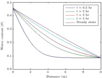
Figure 2. Water content distribution for the analytical solution (Eq. (9)) at t = 0:5; 2; 3; 5 hrs and the steady state.
Obviously, Eq. (9) satises Eq. (7) and the boundary and initial conditions therein. The rst term in Eq. (9), the unsteady term, consists of an exponen-tial expression (with a negative power) in an innite series. At early times, both V and W contribute to spatiotemporal water content distribution. However, at later times (as t ! 1), V vanishes quickly, and W (x), the steady state term, would be the solution. A plot of Eq. (9) is shown in Figure 2 for the following soil parameters:
L= 0:458; r= 0:086;
D = 4mhr2; L = 10 m:
As shown, water content prole reects the unsteady advancing front, which eventually ends up in a linear steady state. Figure 3(a) and (b) show comparisons of a Finite-Dierence Method (FDM) solution (to Eq. (7)) by implicit scheme, with the analytical solution for t = 0:5 hr and t = 3 hr, respectively. The FDM solution was obtained for t = 6 min and x = 0:2 m. As shown, both solutions coincide well with one another.
4. Analytical solution for 1D vertical water inltration
Richards' equation for 1D vertical ow (z direction) with constant 0 at the top boundary would be:
@ @t = D
@2
@z2 + f
@
@z (10)
Figure 3. Comparison of water content proles for the analytical solution (Eq. (9)) and a Finite-Dierence Method (FDM): (a) 0.5 hr and (b) 3 hr.
Figure 4. Schematic view of 1D vertical inltration problem (z direction).
The boundary and initial value problem is shown schematically in Figure 4.
Again, an analytical solution is sought whereby both steady and unsteady solutions may be obtained from a single closed form solution. The general form of the equation is expressed again as a combination of a steady (W ) and an unsteady (V ) term:
(z; t) = V (z; t) + W (z): (11) Substituting Eq. (11) into Eq. (10) and using separa-tion of variables for (z; t) yields:
(z; t) =e 2Df z 4Df2t
1
X
n=1
A
nsinnL z
e (nL)2Dt
+ Qe Dfz+ P; (12)
where A
n, P , and Q are:
A n=L2
Z L
0
(r P )e2Df z Qe 2Df z
sinnLzdz =L2
(r P ) e
f 2DL n
L
( 1)n+ n L
f 2D
2
+ n L
2
Q e
f 2DL n
L
( 1)n+ n L
f 2D
2
+ n L
2
; (13)
P = re
f DL 0
1 + e DfL ;
Q = (0 r) 1 + e DfL:
Obviously, Eq. (12) satises Eq. (10) and the boundary and initial conditions therein. The rst term in Eq. (12), the unsteady term, consists of two exponential expressions in t and z (with negative powers) in and out of an innite series. The steady term, W , has also an exponential expression in z. At early times, both V and W contribute to spatiotemporal water content distribution. However, at later times (as t ! 1), V vanishes quickly, and W (z), the steady state term, would be the solution. A plot of the analytical solution (Eq. (12)) is shown in Figure 5 for the following soil parameters:
0= 0:3; r= 0:0286; s= 0:3658;
L = 100 cm; = 0:01 1
cm; Ks= 10 3 cm
s : As shown, water content proles reect the unsteady inltrating front with constant water contents at the top and bottom of the column (0 = 0:3 and
r= 0:0286, respectively), which eventually ends up in
Figure 5. Water content distribution for the analytical solution (Eq. (12)) for various times.
as time elapses, the proles approach steady state, and their temporal variation (advancement) approaches zero.
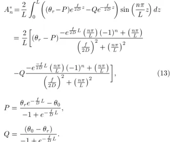
Figure 6(a) and (b) show comparisons of a Finite-Dierence Method (FDM) solution (to Eq. (10)) by implicit scheme with the analytical solution for t = 5 min and t = 10 min, respectively. The FDM solution was obtained for t = 1 min and z = 5 cm. As shown, both solutions coincide well with one another.
A dierent boundary condition may be as-sumed for the 1D vertical water inltration problem (Eq. (10)), whereby an initially \dried" soil column, (z; 0) = r, is subjected to a xed water content at
z = 0 and z = L; (0; t) = (L; t) = 0 > r, thus
allowing the column to imbibe water from both ends. Following similar mathematical procedure as before, the answer for (z; t) would be:
(z; t) = e 2Df z 4Df2t
1
X
n=1
2
L(r 0)
e2Df L n
L
( 1)n+ n L
f 2D
2
+ n L
2 sin
n L z
e (nL)2Dt+0: (14)
Obviously, Eq. (14) satises Eq. (10) and the afore-mentioned boundary and initial conditions. The rst term in the equation, the unsteady term, consists of two exponential expressions in t and z (with negative powers) in and out of an innite series. It reects the spatiotemporal water content distribution in the column above and over the xed water content at both ends of the column, 0. Justiably, it vanishes as
t ! 1 and only the second term in the equation, the steady term W = 0, would be the solution. A plot
of the solution (Eq. (14)) is shown in Figure 7 for the following soil parameters:
0= 0:3; r= 0:0286; s= 0:3658;
L = 1000 cm; = 0:01cm1 ; Ks= 10 3cms :
As shown in the gure, water content proles reect a combination of two unsteady fronts due to the high water content gradient at the top and bottom of the column. The rst one is an inltrating front from top to bottom, and the second is an imbibed front from bottom to top of the column. Perceptibly, gravity eect expedites advancement of the former and impedes that of the latter; an eect that makes the overall water content proles asymmetric unless at the steady state where a constant water content (0) is achieved
throughout the column.
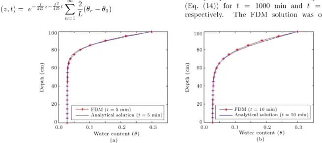
Figure 8(a) and (b) show comparisons of the Finite-Dierence Method (FDM) solution to the prob-lem by implicit scheme, with the analytical solution (Eq. (14)) for t = 1000 min and t = 1500 min, respectively. The FDM solution was obtained for
Figure 6. Comparison of water content proles obtained by the analytical and FDM solutions to Eq. (10) for (a) t = 5 min and (b) t = 10 min.
Figure 7. Water content prole at dierent times for the analytical solution presented in Eq. (14).
t = 5 min and z = 10 cm. As shown, both solutions coincide well with one another.
5. Analytical solution for 2D water inltration Richards' equation in a vertical 2D plane (x; z) may be expressed as (see Eq. (5)):
@ @t = D
@2
@z2+ f
@ @z + D
@2
@x2; (15)
where D and f are dened before. If vertical water inltration from the top edge of the plane is considered, then the initial and boundary conditions would be:
(0; z; t) = r; (a; z; t) = r; (16a)
(x; 0; t) = r; (x; b; t) = 0; (16b)
(x; z; 0) = r; (16c)
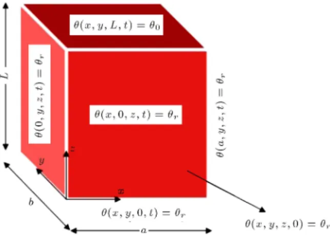
where 0 > r, and a schematic view of the problem
statement is shown in Figure 9. A single closed form analytical solution is sought that encompasses both steady and unsteady solutions. Thus, the general form of such a solution may be expressed as a combination of a steady (W ) and an unsteady (V ) term:
(x; z; t) = V (x; z; t) + w(x; z): (17) Obviously, non-homogenous boundary conditions are to satisfy w(x; z), the steady solution, and homogenous boundary conditions are for V (x; z; t), the unsteady solution. Substituting Eq. (17) into Eqs. (15) and (16a) to (16c) yields:
Figure 9. Schematic view of vertical inltration in a 2D (x; z) plane.
Figure 8. Comparison of water content proles obtained by the analytical (Eq. (14)) and FDM solutions for (a) t = 1000 min and (b) t = 1500 min.
D@2V @z2 + f
@V @z + D
@2V
@x2
@V
@t = 0; (18a) V (x; 0; t) = 0 V (x; b; t) = 0; (18b)
V (0; z; t) = 0 V (a; z; t) = 0; (18c)
V (x; z; 0) = r w(x; z): (18d)
Similarly, the PDE for w(x; z) may be written as:
D@@z2w2 + f@w@z + D@@x2w2 = 0; (19a)
w(x; 0) = r w(x; b) = 0; (19b)
w(0; z) = r w(a; z) = r: (19c)
If w(x; z) is assumed to have two components as follows:
w(x; z) = u(x; z) + q(z); (20) then, the PDE for u(x; z) and q(z) may be written as follows:
Dq00+ fq0= 0; (21a)
q(b) = 0; q(0) = r; (21b)
D@@z2u2 + f@u@z+ D@@x2u2 = 0; (22a)
u(x; 0) = 0; u(x; b) = 0; (22b)
u(0; z) = r q(z); u(a; z) = r q(z): (22c)
By changing variable u(x; z) = e 2Df zN(x; z) and
uti-lizing separation of variables for N(x; z), then w(x; z) would be:
w(x; z) =e 2Df z
1
X
n=1
sinn
b z Ansinh( p
h + 2x)
+ Bncosh(
p
h + 2x)
+re
f Db 0
1 + e Dfb
+(0 r)e
f Dz
1 + e Dfb ; (23)
where = n
b , n = 1; 2; 3; :::; 1, and h = 14f
2
D2. Also,
An and Bn are dened as follows:
Bn=2b
Z b
0
(r P1)e2Df z Q1:e 2Df z
sinnb zdz = 2b
(r P1)
: e
f 2Db n:
b
( 1)n+ n: b
f 2D
2 + n:
b
2
Q1: e
f 2Db n:
b
( 1)n+ n: b
f 2D
2
+ n: b
2
; (24a)
An= sinh(pBh + n 2a)
1 cosh(ph + 2a)
; (24b) where P1and Q1 are:
P1= re
f Db 0
1 + e Dfb ; Q1=
(0 r)
1 + e Dfb: (25)
Utilizing separation of variables for V (x; z; t) as follows: V (x; z; t) = Z(z)X(x)T (t); (26) and substituting Eq. (26) into Eq. (18a), one would get:
X00
X = Z00
Z f D
Z0
Z + 1 D
T0
T = ; (27)
where is an arbitrary constant. If < 0, say = 2, > 0, then considering the boundary conditions
of Eq. (18c), X(x) in Eq. (27) may be written as: Xi= Ai sin(; x); =ia; i = 1; 2; 3; :::; 1; (28)
where A
i is a constant. Substituting 2into Eq. (27)
for X00
X yields:
Z00
Z f D
Z0
Z = 2 1 D
T0
T = ; (29)
where is an arbitrary constant. If 0, then a trivial solution to Z(z) in Eq. (29) would be obtained. If < 0, say = 2 f
D
2 1
4, > 0, then applying the
boundary condition of Eq. (18b) into Eq. (29) would yield Z(z) as follows:
Zm= Cme
f
2Dzsin(z); = m
b ;
m = 1; 2; 3; :::; 1; (30) where C
mis a constant. In addition, T (t) into Eq. (29)
T = B mie
2+2+(f D)2 14
Dt; (31)
where B
miis a constant. Substituting Eqs. (28), (30),
and (31) into Eq. (26) yields:
V (x; z; t) =X1
m=1 1
X
i=1
Cmie 2Df zsin(z)
sin(x)e
2+2+(f D)2 14
Dt; (32)
where Cmi is AiCmBmi . Substituting the boundary
condition of Eq. (18d) into Eq. (32) and using Fourier series properties for Eq. (32), Cmi is calculated by
Eq. (33) as shown in Box I, where Am and Bm
are identical to An and Bn in Eqs. (24a) and (24b),
respectively. Substituting Eqs. (23) and (32) into Eq. (17), (x; z; t) would be:
(x; z; t) =
1
X
m=1 1
X
i=1
Cmie 2Df zsin(z) sin(x)
e
2+2+(f D2)14
Dt+ e f 2Dz
:X1
n=1
sinnb z Ansinh(
p
h + 2x)
+ Bncosh
p
h + 2x+(0 r):e
f Dz
1 + e Dfb
+r:e
f Db 0
1 + e Dfb : (34)
As seen, the equation consists of four terms: a function of (x; z; t), a function of (x; z), a function of z only, and a constant. As t ! 1, the rst term vanishes, and the rest of the terms remain as residuals or the steady state solution. Based on the equation, water content contours are drawn in Figure 10(a) to (d) for t = 5; 15; 30; and 60 min, respectively. Figures are generated for the following soil parameters:
a = 100 cm; b = 100 cm; 0= 0:3;
r= 0:0286; s= 0:365;
= 0:01cm1 ; Ks= 10 3cms :
Graphs in Figure 10 clearly show the inltrating water content front that remains at 0 = 0:3 at the top of
soil sample (z = 100 cm) and at the residual value of r = 0:0286 at the bottom of the sample (z = 0). In
addition, water content contours at x = 0 and x = 100 cm remain at r= 0:0286 all the times. 3D plots
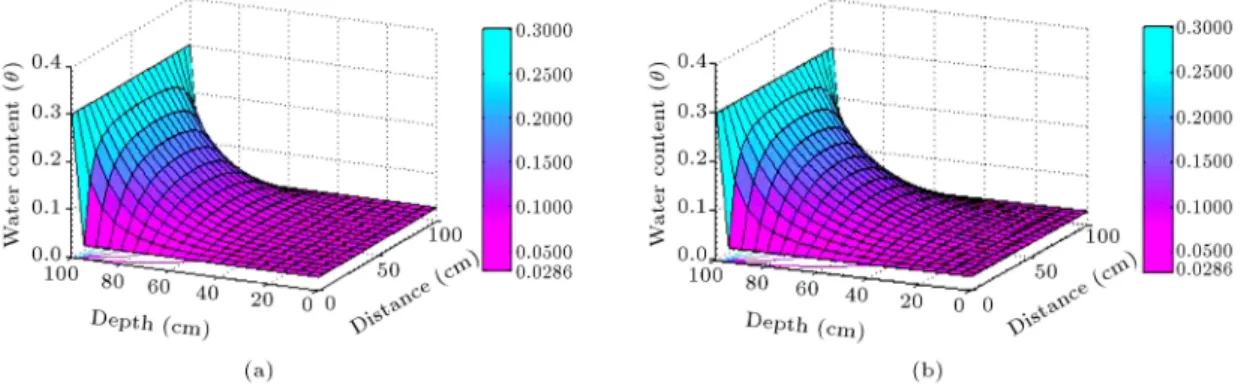
of water content, water depth, and water distance for t = 30 and 60 min (corresponding to Figure 10(c) and (d)) are visualized in Figure 11(a) and (b), respectively. Comparison of Figure 11(a) and (b) clearly depicts a 3D view of the inltrating water content front.
6. Analytical solution for 2D water inltration with no-ow on the side boundaries and a constant initial condition
Boundary and initial conditions may be applied to Eq. (15), such that a no-ow boundary condition is implemented on certain sides of the domain. No-ow
Cmi= ab4 Z a
0 Z b
0
re2Df z w(x; z)e2Df z
sin(z) sin(x)dzdx
= ab4 2b
Am iasinh q
h + m b
2a( 1)i+ B
m ia ( 1)i+1cosh q
h + m b
2a+ 1 h + m
b
2+ i a
2
!
4rmba
1 + ( 1)i+ ebf
2D ( 1)m ( 1)m+i
fb D
2
+ 42m2
i 4mba
Q1 1+( 1)i+1+P1 1+( 1)i+1+Q1e2Dbf ( 1)m+1+( 1)m+i+P1e2Dbf ( 1)m+1+( 1)m+i
fb D
2
+42m2
i
! (33) Box I
Figure 10. Water content contours based on the analytical solution to Eq. (34) for (a) t = 5 min, (b) t = 15 min, (c) t = 30 min, and (d) t = 60 min.
Figure 11. 3D plots of water content, water depth, water distance based on the analytical solution to Eq. (34) for (a) t = 30 min and (b) t = 60 min.
boundary conditions at x = 0 and x = a and constant boundary conditions at z = 0 and z = b along with a constant initial condition are mathematically written as follows:
@
@x(0; z; t) = 0; @
@x(a; z; t) = 0; (35a) (x; 0; t) = r; (x; b; t) = 0; (35b)
(x; z; 0) = r: (35c)
(x; z; t) may be divided into two terms as:
(x; z; t) = V (x; z; t) + w(z): (36)
Replacing Eq. (36) into Eqs. (15) and (35) and con-sidering the non-homogenous boundary (Eq. (35b)) for w(z), one would obtain:
w(z) = P1+ Q1e Dfz;
P1= re
f Db 0
1 + e Dfb ;
Q1= (0 r)
1 + e Dfb: (37)
V (x; z; t) may be expressed via separation of variables as follows:
Substituting Eq. (38) into Eq. (15) and applying some simplications gives: X00 X = Z00 Z + f D Z0 Z 1 D T0 T
= ; (39)
where is an arbitrary constant. If = 0 and < 0, say = 2and > 0, then X(x) has two answer:
X = B; (40)
Xn = Ancos(x); = na ; n = 1; 2; 3; :::; 1;
(41) where B and A
n are constants. Substituting = 0
and = 2 into Eq. (39) for X00
X , two equations are
obtained: 2= Z00
Z + f D Z0 Z 1 D T0 T ; (42a) 0 = Z00 Z + f D Z0 Z 1 D T0 T : (42b)
Considering Eqs. (35b) and (36), homogeneous bound-aries for V (x; z; t) based on Eq. (42a) gives:
Zm= Bme
f
2Dzsin(vz); v =m
b ;
m = 1; 2; 3; :::; 1; (43) T (t) = C
mne (
2+v2+(f
D)2 14)Dt; (44)
where B
m and Cmn are constants. Substituting
Eqs. (41), (43), and (44) into Eq. (38), an answer for V (x; z; t) would be derived as:
V1(x; z; t) = 1 X m=1 1 X n=1
Cmncosna x
sinmb z e 2Df ze (2+v2+(Df)2 14)Dt; (45)
where Cmn is AnBmCmn .
A similar procedure may be followed to obtain Z(z) and T (t) in Eq. (42b):
Zm= Ame
f
2Dzsin(z); = m
b ;
m = 1; 2; 3; :::; 1; (46) T = B
ie (
2+(f
D)2 14)Dt; (47)
where A
m and Bi are constants. Substituting
Eqs. (40), (46), and (47) into Eq. (38), another answer would be obtained for V (x; z; t):
V2(z; t) = 1
X
m=1
Cme
f
2Dzsinm
b z
e (2+(f D)2 14)Dt;
(48)
where Cm is BAmBi. Now, V (x; z; t) may be written
as a combination of Eqs. (45) and (48):
V (x; z; t) =V1(x; z; t) + V2(z; t) = 1 X m=1 1 X n=1 Cmn
cosna xsinmb z e 2Df ze (2+v2+(Df)2 14)Dt
+X1
m=1
Cme
f
2Dzsinm
b z
e (2+(f
D)2 14)Dt: (49)
Substituting Eq. (36) into Eq. (35c) and replacing the result into Eq. (49), along with application of some Fourier series properties, would yield Cmn and Cm as
follows: Cmn=ab4
Z b 0 Z a 0 e f 2Dz
r P1 Q1:e Dfz
sinm b z cosn a x
dxdz ! Cmn= 0;
(50a)
Cm=ab2
Z b 0 Z a 0 e f 2Dz
r P1 Q1:e Dfz
sinmb zdxdz = 2b :
(r P1): e
f 2Db m:
b
( 1)m+ m: b f 2D 2 + m: b 2
Q1: e
f 2Db m:
b
( 1)m+ m: b f 2D 2 + m: b 2 : (50b) Substituting Eqs. (49) and (37) into Eq. (36) gives:
(x; z; t) =X1
m=1
Cme 2Df zsinm
b z
e (2+(f D)14)Dt
+ P1+ Q1:e
f
Dz: (51)
Eq. (51) is independent of x and reects a 1D vertical inltration equation for z and t that is identical to Eq. (12) if b = L.
Figure 12(a) and (b) depict water content con-tours for Eq. (51) at t = 900 and 3600 s. Soil parameters used for the problem are identical to those used in Section 5. As shown, inltrating front forms horizontal lines, which advance as the time increases until they reach the steady state (Figure 12(b)).
Figure 12. Vertically inltrating water content contours plotted based on Eq. (51) for (a) t = 900 s and (b) t = 3600 s. 6.1. Analytical solution to 2D water
inltration with no-ow on the side boundaries and a sinusoidal initial condition
The only dierence in this section (compared to the previous one) is the sinusoidal initial condition over the 2D domain, which may be mathematically expressed as:
(x; z; 0) = 0sinxa
sinz
b
: (52)
Thus, initial condition for V (x; z; 0) would be: V (x; z; 0) = 0sinxa
sinzb w(z): (53) Substituting Eq. (53) into Eq. (49), Cmn may be
calculated by Eq. (54) as shown in Box II. Also, Cm
in Eq. (49) would be obtained by Eq. (55) as shown in Box III. Finally, substituting Eqs. (49) and (37) into Eq. (36) yields:
(x; z; t) =
1
X
m=1 1
X
n=1
Cmncosna x
sinmb z e 2Df ze (2+v2+(Df)2 14)Dt+
1
X
m=1
Cm
e 2Df zsinm
b z
e (2+(f D)2 14)Dt
+ Q1:e Dfz+ P1: (56)
The rst two terms in Eq. (56) are functions of x; z and t, reecting unsteady behavior of the inltrating
Cmn= ab4 Z b
0 Z a
0 e
f 2Dz
0sinxa
sinzb P1 Q1:e
f Dz
cosna xsinmb zdxdz = 80
Hb2m 1+eHb( 1)m
H4b4+2H2b22(1+m2)+4 24m2+4m4
(1+( 1)n) (n2 1)
; for n 6= 1; (54)
where H =2Df and Cmn= 0 if n = 1.
Box II
Cm=ab2 Z b
0 Z a
0 e
f 2Dz
0sinxa
sinzb P1 Q1:e Dfz
sinmb zdxdz = 2
0 2Hb
2m 1 + eHb( 1)m
H4b4+ 2H2b22(1 + m2) + 4 24m2+ 4m4 2 + P1
m 1 + eHb( 1)m H2b2+ m22 Q1m e
Hb ( 1)me Hb H2b2+ m22
: (55)
Figure 13. Water content contours for 2D water inltration with no-ow on the side boundaries and a sinusoidal initial condition for (a) t = 5 min, (b) t = 10 min, (c) t = 15 min, and (d) t = 60 min.
water content front. However, the last two terms are not functions of time and reect the steady behavior of the front. Obviously, as t ! 1, the rst two terms vanish and the solution approaches that of a 1D vertical steady inltration presented by the last two terms in Eq. (12).
Figure 13(a) to (d) depict water content contours for equation Eq. (56) for t = 5; 10; 15 and 60 min, respectively. Soil parameters used for the problem are identical to those used in Section 5. At early times (Figure 13(a) and (b)) water content contours reect a combination of two distinct water content gradients: 1) from center of the domain outward due to the sinusoidal initial bell shape gradient, and 2) from top to bottom (the inltrating front) due to the gradient in water contents at top and bottom boundaries. As time elapses, the bell shape gradient attenuates, the 1D vertical inltration prevails (Figure 13(c) and (d)), and eventually water content contours approach a steady state exponential prole associated with the last two terms in Eq. (56).
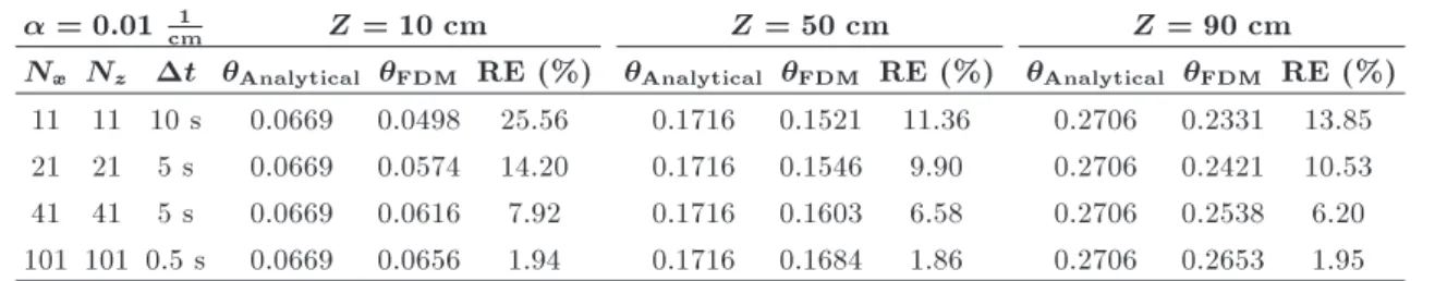
To illustrate the use of the derived equations, water content values from the analytical solution (Eq. (56)) is compared to an explicit scheme Finite Dierence Method (FDM) solution (to Eq. (15) with boundary conditions (Eqs. (35a) and (35b)) and initial condition (Eq. (52))) in Tables 1-4. The soil properties for both solutions are:
a = 100 cm; b = 100 cm; 0= 0:3;
r= 0:0286; s= 0:3658; Ks= 10 3cms :
The tables are for four values of 0:01; 0:0075; 0:005, and 0:0025 1
cm, utilized by Tracy [16], too. The
comparison is performed for t = 30 min, x = 50 cm, z = 10, 50 and 90 cm. The comparison is made for dierent numbers of grid point at x direction (Nx), z
direction (Nz), and time steps (t). Relative Error
(RE) dened as:
RE = jAnalyticalj Numericalj
Analyticalj 100%;
was used as the index for comparison.
As expected, for all 's, RE decreased consider-ably when Nx, and Nz increased (and the time step
(t) decreased to guarantee numerical stability), such that for the highest number of grid points at x and z directions (Nx = Nz = 101) RE is less than 2%.
However, as increased, RE increased, too. Spatially, for all 's, RE at z = 50 cm was less than that at z = 10 and 90 cm for almost all Nx and Nz values.
Apparently, to lower RE at z = 10 and 90 cm, it is necessary to rene the grids near top and bottom boundaries. Similar trends were observed by Tracy [16] for h-based Richards' equation. As he stated, these
Table 1. Comparisons of analytical with FDM solutions for various Z's at x = 50 cm, t = 30 min, and = 0:0025 1 cm.
= 0:0025 1
cm Z = 10 cm Z = 50 cm Z = 90 cm
Nx Nz t Analytical FDM RE (%) Analytical FDM RE (%) Analytical FDM RE (%)
11 11 10 s 0.0577 0.0528 8.49 0.1692 0.1562 7.68 0.2747 0.2501 8.95 21 21 3 s 0.0577 0.0532 7.79 0.1692 0.1574 6.97 0.2747 0.2564 6.66 41 41 1 s 0.0577 0.0561 2.77 0.1692 0.1643 2.89 0.2747 0.2646 3.67 101 101 0.1 s 0.0577 0.0569 1.38 0.1692 0.1672 1.18 0.2747 0.2708 1.41 Table 2. Comparisons of analytical with FDM solutions for various Z's at x = 50 cm, t = 30 min, and = 0:005 1
cm.
= 0:005 1
cm Z = 10 cm Z = 50 cm Z = 90 cm
Nx Nz t Analytical FDM RE (%) Analytical FDM RE (%) Analytical FDM RE (%)
11 11 10 s 0.0586 0.0514 12.28 0.1680 0.1534 8.69 0.2741 0.2481 9.48 21 21 5 s 0.0586 0.0534 8.87 0.1680 0.1553 7.55 0.2741 0.2534 7.55 41 41 2.5 s 0.0586 0.0568 3.07 0.1680 0.1624 3.33 0.2741 0.2621 4.37 101 101 0.3 s 0.0586 0.0577 1.53 0.1680 0.1656 1.42 0.2741 0.2695 1.67 Table 3. Comparisons of analytical with FDM solutions for various Z's at x = 50 cm, t = 30 min, and = 0:0075 1
cm.
= 0:0075 1
cm Z = 10 cm Z = 50 cm Z = 90 cm
Nx Nz t Analytical FDM RE (%) Analytical FDM RE (%) Analytical FDM RE (%)
11 11 10 s 0.0618 0.0501 18.93 0.1685 0.1521 9.73 0.2725 0.2414 11.41 21 21 5 s 0.0618 0.0534 13.59 0.1685 0.1548 8.13 0.2725 0.2501 8.22 41 41 2.5 s 0.0618 0.0581 5.98 0.1685 0.1596 5.28 0.2725 0.2591 4.91 101 101 0.5 s 0.0618 0.0608 1.61 0.1685 0.1656 1.72 0.2725 0.2676 1.79 Table 4. Comparisons of analytical with FDM solutions for various Z's at x = 50 cm, t = 30 min, and = 0:01 1
cm.
= 0:01 1
cm Z = 10 cm Z = 50 cm Z = 90 cm
Nx Nz t Analytical FDM RE (%) Analytical FDM RE (%) Analytical FDM RE (%)
11 11 10 s 0.0669 0.0498 25.56 0.1716 0.1521 11.36 0.2706 0.2331 13.85 21 21 5 s 0.0669 0.0574 14.20 0.1716 0.1546 9.90 0.2706 0.2421 10.53 41 41 5 s 0.0669 0.0616 7.92 0.1716 0.1603 6.58 0.2706 0.2538 6.20 101 101 0.5 s 0.0669 0.0656 1.94 0.1716 0.1684 1.86 0.2706 0.2653 1.95 results demonstrate the usefulness of having analytical
solutions to test numerical programs.
7. Analytical solution for 3D water inltration Richards' equation for 3D water inltration in an isotropic homogeneous Cartesian coordinate system is (see Eq. (5)):
@ @t = D
@2
@x2 + D
@2
@y2 + D
@2
@z2 + f
@
@z; (57) where D and f are dened earlier. A rectangular cube may be considered as the domain. Water inltration would be triggered by a constant but higher water content on the top surface of the cube compared to the remainder of the domain. Boundary and initial
conditions for such a case would be:
(0; y; z; t) = r; (a; y; z; t) = r; (58a)
(x; 0; z; t) = r; (x; b; z; t) = r; (58b)
(x; y; 0; t) = r; (x; y; L; t) = 0; (58c)
(x; y; z; 0) = r: (58d)
A schematic view of the problem statement is shown in Figure 14.
(x; y; z; t) may be considered as a combination of two terms: a steady (w) and an unsteady (V ) one:
(x; y; z; t) = V (x; y; z; t) + w(x; y; z): (59) As mentioned, the non-homogeneous boundary con-ditions are satised by w(x; y; z), the steady state
Figure 14. Schematic view of 3D inltration problem in a cubical domain.
term, and homogeneous boundary conditions are set for V (x; y; z; t), the unsteady state term. Substituting Eq. (59) into Eq. (57) and Eq. (58a) to Eq. (58d) yields:
D@2V @z2 + f
@V @z + D
@2V
@x2 + D
@2V
@y2
@V
@t = 0; (60a) V (0; y; z; t) = 0 V (a; y; z; t) = 0; (60b) V (x; 0; z; t) = 0 V (x; b; z; t) = 0; (60c) V (x; y; 0; t) = 0 V (x; y; L; t) = 0; (60d) V (x; y; z; 0) = r w(x; y; z); (60e)
and:
D@@z2w2 + f@w@z + D@@x2w2 + D@@y2w2 = 0; (61a)
w(0; y; z) = r w(a; y; z) = r; (61b)
w(x; 0; z) = r w(x; b; z) = r; (61c)
w(x; y; 0) = r w(x; y; L) = 0: (61d)
If w(x; y; z) is, in turn, considered as two separate terms:
w(x; y; z) = u(x; y; z) + N(x; y); (62) then, substitution of Eq. (62) into Eqs. (61a) to (61d) yields:
@2N
@x2 +
@2N
@y2 = 0; (63a)
N(0; y) = r N(a; y) = r; (63b)
N(x; 0) = r N(x; b) = r: (63c)
As a simple example for the solution to Eqs. (63a) to (63c), one may consider N(x; y) = r.
Also, the partial dierential equation for u(x; y; z) would be written as:
D@z@2u2 + f@u@z + D@x@2u2+ D@@y2u2 = 0; (64a)
u(0; y; z) = 0 u(a; y; z) = 0; (64b) u(x; 0; z) = 0 u(x; b; z) = 0; (64c) u(x; y; 0) = 0 u(x; y; L) = 0 r= r0: (64d)
Applying separation of variables to u(x; y; z):
u(x; y; z) = X(x)Y (y)Z(z); (65) and substituting Eq. (65) into Eq. (64a), while using Eqs. (64b) and (64c) we obtain:
Yn=Ansin(y); =nb ; n=1; 2; 3; :::; 1; (66)
Xm= Bm sin(x); = m:a ; m = 1; 2; 3; :::; 1;
(67) where A
n and Bm are constants. Similarly, Z(z) in
Eq. (65) becomes:
Z = e 2Dfz C1ez+ C2e z;
= s
1 4
f D
2
+ (2+ 2); (68)
where C
1 and C2 are constants. Eq. (68) may be
further simplied as:
Z = C mne
fz
2Dsinh(z) + Bmn e 2Dfz cosh(z): (69)
Applying the boundary condition of Eq. (64d), u(x; y; 0) = 0 to Eq. (69) gives:
Z = C mne
fz
2Dsinh(z); (70)
where C
mnis a constant. Substituting Eqs. (66), (67),
and (70) into Eq. (65) would give:
u(x; y; z)=X1
m=1 1
X
n=1
Cmne
f
2Dzsinh(z)
sin(x) sin(y); (71)
u(x; y; L) = 0 r= 0rand Fourier series properties,
Cmn in Eq. (71) would be obtained as:
Cmn= ab4
Z b 0 Z a 0 0 re f 2DL
sinh(L)sin(x) sin(y)dxdy
= 40re
f 2DL
sinh(L)
1 ( 1)n ( 1)m+ ( 1)m+n
mn2 :
(72) As stated in Eq. (62), one may readily add up Eq. (71) and N(x; y) = r, to get w(x; y; z).
Separation of variables may also be applied to V (x; y; z; t) in Eq. (60):
V (x; y; z; t) = X(x)Y (y)Z(z)T (t): (73) Substituting Eq. (73) in Eq. (60a), simplication, and applying Eqs. (60b), (60c) and (60d) one would obtain:
Xi= Ai sin(x); = i:a i = 1; 2; 3; :::; 1; (74a)
Yi= Bjsin(y); = j:b j = 1; 2; 3; :::; 1; (74b)
Zk= Cke
f
2Dzsin(vz); v =k
L;
k = 1; 2; 3; :::; 1; (74c)
T = F ijke (
2+2+v2+(f
D)2 14)Dt; (74d)
where A
i, Bj, Ck, and Fijk are constants. Substituting
Eqs. (74a), (74b), (74c) and (74d) into Eq. (73) gives:
V (x; y; z; t) =
1 X i=1 1 X j=1 1 X k=1
Cijksin
i ax sin j b y sin k L z e 2Df ze
2+2+v2+(f D2)14
Dt;
(75) where Cijk is AiBjCkFijk . Substituting the initial
condition of Eq. (60e) into Eq. (75) and considering Fourier series properties, Cijk may be obtained as:
Cijk =abL8
Z L 0 Z b 0 Z a 0
re2Df z w(x; y; z)e2Df z
sin i ax sin j b y sin k L z dxdydz
= L2 C ij
k L
( 1)ksinh(L)
2+ k L
2 ;
(76)
where and C
ij are dened as:
= s 1 4 f D 2 + i a 2 + j b 2 ; (77) C ij = 4
0 re
f 2DL
sinh(L)
1 ( 1)j ( 1)i+ ( 1)j+i
ji2 :
(78) Substituting Eqs. (62) and (75) into Eq. (59) yields:
(x; y; z; t) =X1
i=1 1 X j=1 1 X k=1
Cijksin
i ax sin j b y sin k Lz
e 2Df ze (2+2+v2+(Df)2 14)Dt
+ 1 X m=1 1 X n=1
Cmne 2Df zsinh(z) sinm
a x
sinnb y+ r; (79)
which gives the spatiotemporal variations of water content in the cube of Figure 14, and is considered as the exact analytical solution for Eq. (57). All boundary and initial conditions of Eqs. (58a) to (58d), as well as Eq. (57), are satised by Eq. (79). The rst term in Eq. (79) is the unsteady state term, it vanishes as t ! 1 (due to the second exponential expression), and the second and third terms remain as the residual or steady state terms. Problem statement dictates symmetrical water content proles over two sections of 1) x = a=2 and 2) y = b=2; a fact that is incorporated in Eq. (79) due to the sinusoidal x and y terms. Furthermore, as the higher water content contours inltrate into the cube as a \front", maximum advancement of the \front" always lays along the line of (a=2; b=2; z).
To plot numerical examples for Eq. (79), the following soil parameters were selected:
a = 100 cm; b = 100 cm; L = 100 cm; 0= 0:3; r= 0:0286; s= 0:3658;
= 0:01cm1 ; Ks= 10 3cms :
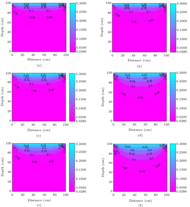
Figure 15(a) to (f) depict two dimensional (x; z) water content contours at vertical sections of y = 10; 25 and 50 cm at t = 15 and 60 min. As shown, the boundary conditions of Eq. (58a) to (58c) are all satised; r = 0:0286 is xed at x = 0; 100 cm
and z = 0 cm and 0 = 0:3 xed at z = 100 cm.
Figure 15. Water content contours for the 3D analytical solution presented in Eq. (79) for (a) y = 10 cm and t = 15 min, (b) y = 10 cm and t = 60 min, (c) y = 25 cm and t = 15 min, (d) y = 25 cm and t = 60 min, (e) y = 50 cm and t = 15 min, (f) y = 50 cm and t = 60 min.
and (e)) to those for t = 60 min (Figure 15(b), (d), and (f)), clearly shows temporal advancement of the vertically inltrating front of water content from top (z = 100 cm) to bottom (z = 0 cm) of the cube at dierent sections. Comparing gures for y = 10; 25, and 50 cm reects the fact that at higher y values (sections closer to the center of the cube), deeper inltration of water content contours occurs, with the maximum advancement laying on the vertical line passing through the center of the cube. Finally, it was noted that at t = 60 min, contribution of the rst, compared to the second and third terms in Eq. (79) was negligible; as if steady state was reached at this time.
8. Analytical solution for 3D water inltration with no-ow on the side boundaries and a constant initial condition
Dierent boundary and initial conditions may be con-sidered for Eq. (57). For example, no-ow may be considered on the side boundaries with higher water content on the top surface of the cube (compared to the remainder of the domain) triggering vertical inltration of water content. Mathematical expression for such boundary and initial conditions would be:
@
@x(0; y; z; t) = 0; @
@
@y(x; 0; z; t) = 0; @
@y(x; b; z; t) = 0; (80b) (x; y; 0; t) = r; (x; y; L; t) = 0; (80c)
(x; y; z; 0) = r: (80d)
As before, (x; y; z; t) is considered as:
(x; y; z; t) = V (x; y; z; t) + w(z): (81) Substituting Eq. (81) into Eq. (57) and applying the boundary condition of Eq. (80c), w(z) becomes:
w(z) = P + Qe Dfz; P = r:e f DL 0
1 + e f DL ;
Q = (0 r)
1 + e DfL: (82)
The PDE for V (x; y; z; t) is the same as Eq. (60a), how-ever, with dierent boundary and initial conditions:
@V
@x(0; y; z; t) = 0; @V
@x(a; y; z; t) = 0; (83a) @V
@y(x; 0; z; t) = 0; @V
@y(x; b; z; t) = 0; (83b) V (x; y; 0; t) = 0; V (x; y; L; t) = 0; (83c) V (x; y; z; 0) = r w(z); (83d)
V (x; y; z; t) may be separated as:
V (x; y; z; t) = X(x)Y (y)Z(z)T (t): (84) Substituting Eq. (84) into Eq. (60a) and applying some simplications give: X00 X = Z00 Z + f D Z0 Z + Y00 Y 1 D T0 T
= ; (85) where is an arbitrary constant. If = 0 and < 0, say = 2, > 0 then X(x) in Eq. (85) has two
answers as:
X1= B; (86)
Xn= Ancos(x); = n:a ; n = 1; 2; 3; :::; 1;
(87) where B and A
n are constants. If > 0, then a trivial
solution would be obtained for X(x). Substituting = 0 and = 2 in Eq. (85) for X00
X , two equations are
obtained: 2= Z00
Z + f D Z0 Z + Y00 Y 1 D T0 T ; (88a) 0 = Z00 Z + f D Z0 Z + Y00 Y 1 D T0 T : (88b)
With rearrangements, Eq. (88a) becomes: 2 Z00
Z + f D Z0 Z 1 D T0 T
= YY00 = ; (89) where is arbitrary constant. Applying = 0 and < 0, say = 2, > 0 and boundary conditions of
Eq. (83b), two answers for Y (y) are obtained:
Y1= D; (90)
Ym= Bm cos(y); = m:b ; m = 1; 2; 3; :::; 1;
(91) where D and B
m are constants. Substituting = 0
and = 2 into Eq. (89) for Y00
Y , two equations may
be written as: 2 Z00
Z + f D Z0 Z 1 D T0 T
= 2; (92a)
2 Z00
Z + f D Z0 Z 1 D T0 T
= 0: (92b) Using Eq. (83c) for Eq. (92a) gives:
Z k=Cke
f
2Dzsin(z); =k
L;
k =1; 2; 3; :::; 1; (93) Tmnk = Dmnk e (
2+2+2+(f
D)2 14)Dt; (94)
where C
k and Dmnk are constants. As before,
Eq. (92b) yields: Z
k = Cke
f
2Dzsin(z); = k
L ;
k = 1; 2; 3; :::; 1; (95a) Tnk= Enk e (
2+2+(f
D)2 14)Dt; (95b)
where C
k and Enk are constants. Now, substituting
Eqs. (87), (91), (93) and (94) into Eq. (84), the rst answer for V (x; y; z; t) yields as:
V2(x; y; z; t) = Xn(x)Y1(y)Zk(z)Tnk(t)
=X1
n=1 1
X
k=1
Dnkcosna x
sin k L z
e 2Df ze
2+2+(f D2)14
Dt; (96)
where Cnmk is AnBmCkDmnk. Also, substituting
Eqs. (87), (90), (95a) and (95b) into Eq. (84), the second answer for V (x; y; z; t) may be written as:
= 1 X n=1 1 X k=1
Dnkcosna x
sin k L z e 2Df z
e (2+2+(f
D)2 14)Dt; (97)
where Dnk is AnDCkEnk . As before, Eq. (88b) also
gives two answers for V (x; y; z; t) as:
V3(x; y; z; t) = 1 X m=1 1 X k=1
Amkcosmb y
sin k L z
e 2Df ze (2+2+(Df)2 14)Dt (98)
V4(x; y; z; t) = 1
X
k=1
Bksin
k
L z
e 2Df z
e (2+(f
D)2 14)Dt; (99)
where Amk and Bk are constants. Also = m:b , m =
1; 2; 3; :::; 1, and = k
L, k = 1; 2; 3; :::; 1.
Finally, the overall answer for V (x; y; z; t) is the combination of Eqs. (96) to (99):
V (x; y; z; t) = V1(x; y; z; t) + V2(x; y; z; t)
+V3(x; y; z; t) + V4(x; y; z; t)
=X1
n=1 1 X m=1 1 X k=1
Cnmkcosna x
cosmb ysin
k L z
e 2Df z
e (2+2+2+(f
D)2 14)Dt+
1 X n=1 1 X k=1 Dnk
cosna xsin
k L z
e 2Df z
e (2+2+(f
D)2 14)Dt+
1 X m=1 1 X k=1 Amk
cosmb ysin
k L z
e 2Df z
e (2+2+(f
D)2 14)Dt+
1
X
k=1
Bksin
k
L z
e 2Df ze (2+(Df)2 14)Dt: (100)
Now, substituting Eq. (83d) into Eq. (100) and, apply-ing Fourier series properties yields: Cnmk, Dnk, and
Amk= 0 and only Bk remains as:
Bk =abL2
Z L 0 Z b 0 Z a 0 e f
2Dz(r P Qe Dfz)
sin
k L z
dxdydz = L2:
(r P )
e2Df L k
L
( 1)k+ k L f 2D 2 + k L 2 Q e f 2DL k
L
( 1)k+ k L f 2D 2 + k L 2 : (101)
All constant coecients in Eq. (100) except Bk are
zero. Therefore, 3D no-ow boundary inltration problem with the initial condition of Eq. (80d) is identical to 1D inltration problem. Substituting Bk
into Eq. (100) and using Eq. (81) yields:
(x; y; z; t) =
1
X
k=1
Bksin
k
L z
e 2Df ze (2+(Df)2 14)Dt
+ P + Qe Dfz: (102)
Eq. (102) is exactly the same as Eq. (51) derived for 2D no-ow boundary inltration problem with initial constant water content. Water content contours for Eq. (102) at any constant y section would be similar to those depicted by Figure 12(a) and (b).
8.1. Analytical solution for 3D water inltration with no-ow on the side boundaries and a sinusoidal initial condition
The only dierence in this section (compared to the previous one) is the sinusoidal initial condition over the 3D domain, which may be mathematically expressed as:
(x; y; z; 0) = 0sinxa
sinyb sinzL : (103) Substituting Eq. (103) into Eq. (83d), and then substituting the result into Eq. (100) and applying Fourier series properties give the equations shown in Box IV, where H = 2Df . Using these coecients in Eq. (100) and substitution into Eq. (81) yields Eq. (105) as shown in Box V.
This equation is considered as the exact analytical solution to the problem since it satises the PDE (Eq. (57)), boundary conditions of Eq. (80a) to (80c),
and the initial condition of Eq. (103). The rst four terms in Eq. (105) are functions of x; y; z, and t, reecting unsteady behavior of the inltrating water content front. However, the last two terms are not functions of time, and reect the steady behavior of the front. Obviously, as t ! 1, the rst four terms vanish and the solution approaches that of a 1D vertical steady inltration presented by the last two terms in Eq. (12). Problem statement dictates symmetrical water content proles over two sections of 1) x = a=2 and 2) y = b=2; a fact that is incorporated in Eq. (105) due to the cosine terms in x and y.
Figure 16(a) to (m) depict water content contours plotted using Eq. (105) for t = 5; 10; 15, and 60 min, and for y = 10; 25, and 50 cm. The value of soil parameters used to plot these gures are identical to those used in Section 7. At early times (for all y's; Figure 16(a), (e), and (i) water content contours reect a combination of two distinct water content gradients: 1) from center of the domain outward due to the sinusoidal initial bell shape gradient, and 2) from top to bottom (the inltrating front) due to the gradient in water contents at top and bottom boundaries. As time elapses, the bell shape gradient attenuates, the
Figure 16. Water content contours plotted using Eq. (105) for (a) y = 10 cm and t = 5 min, (b) y = 10 cm and t = 10 min, (c) y = 10 cm and t = 15 min, (d) y = 10 cm and t = 60 min, (e) y = 25 cm and t = 5 min, (f) y = 25 cm and t = 10 min, (g) y = 25 cm and t = 15 min, (h) y = 25 cm and t = 60 min, (i) y = 50 cm and t = 5 min, (j) y = 50 cm and t = 10 min, (k) y = 50 cm and t = 15 min, (m) y = 50 cm and t = 60 min (other parameter values in Eq. (105) are given in the text).
Cnmk==abL8 Z L
0 Z b
0 Z a
0 e
f 2Dz
0sinxa
sinyb sinzL P Qe Dfz
sin
k
Lz
cosna x cosm
b y
dxdydz = 160
HL2k 1 + eHL( 1)k
H4L4+ 2H2L22(1 + k2) + 4 24k2+ 4k4
(1 + ( 1)n) (n2 1)
(1 + ( 1)m) (m2 1)
for n 6= 1 and m 6= 1; if n = 1 or m = 1 ! Cnmk = 0 (104)
Dnk=abL4 Z L
0 Z b
0 Z a
0 e
f 2Dz
0sinxa
sinyb sinzL P Qe Dfz
sin
k
L z
cosna xdxdydz = 80
HL2k 1 + eHL( 1)k
H4L4+ 2H2L22(1 + k2) + 4 24k2+ 4k4
(1 + ( 1)n) (n2 1)
2
for n 6= 1 if n = 1 ! Dnk= 0 Amk=abL4
Z L 0
Z b 0
Z a 0 e
f 2Dz
0sinxa
sinyb sinzL P Qe Dfz
sin
k
L z
cosmb ydxdydz = 80
HL2k 1 + eHL( 1)k
H4L4+ 2H2L22(1 + k2) + 4 24k2+ 4k4
(1 + ( 1)m) (m2 1)
2
for m 6= 1 if m = 1 ! Amk= 0
Bk =abL2 Z L
0 Z b
0 Z a
0 e
f 2Dz
0sinxa
sinyb sinzL P Qe Dfz
sin
k Lz
dxdydz = 2
abL
2HL2k 1 + eHL( 1)k 0
H4L4+ 2H2L22(1 + k2) + 4 24k2+ 4k4 4 2 + P
k 1 + eHL( 1)k H2L2+ k22 Qk eHl ( 1)k
e HL H2L2+ k22
Box IV
1D vertical inltration prevails (Figure 16(d), (h), and (m), and eventually water content contours approach a steady state exponential prole associated with the last two terms in Eq. (105).
Figure 17(a) and (b) show 3D plots of water content contours at y = 50 cm section (middle section of the cubic domain) for t = 5 and 10 min. These gures are actually 3D plots of Figure 16(i) and (j), respectively. Comparison of Figure 17(a) and (b) shows how the initial condition of a \water content hump" in the middle of the cube, and boundary conditions of a sharp water content gradient interact, as the time elapses. As shown, the peak of the \hump" attenuates
while water content near the side boundaries increase and their combination approach the nal steady state water content distribution over the domain.
9. Conclusions
New analytical solutions to Richards' equation in one, two, and three dimensions subject to various boundary and initial conditions were presented using separation of variables and Fourier series expansion techniques. Solutions have the general form of innite series with exponential terms whereby both steady and unsteady solutions may be obtained from a single closed form
so-(x; y; z; t) = 1 X n=1
1 X m=1
1 X k=1
Cnmkcosna x
cosmb ysin
k L z
e 2Df ze (2+2+2+(Df)2 14)Dt
+ 1 X n=1
1 X k=1
Dnkcosna x
sin
k L z
e 2Df ze (2+2+(Df)2 14)Dt
+X1 m=1
1 X k=1
Amkcosmb y
sin
k Lz
e 2Df ze (2+2+(Df)2 14)Dt+
1 X k=1
Bk sin
k
Lz
e 2Df ze (2+(Df)2 14)Dt+ Qe Dfz+ P (105)
Box V
Figure 17. 3D plots of Eq. (105) for y = 50 cm: (a) t = 5 min and (b) t = 10 min (other parameter values in Eq. (105) are given in the text).
lution. Analytical solutions for 1 and 2D horizontal and vertical water inltration were compared to numerical nite dierence method solutions and shown to have less than 2% dierence. Solutions to 2 and 3D vertical water inltration were derived for constant, no-ow, and sinusoidal boundary and initial conditions. The solutions may be utilized to test numerical models that use dierent computational techniques.
References
1. Bear, J. and Chang, A.H., Modeling Groundwater Flow and Contaminant Transport, Springer Interscience Publication (2010).
2. An, H., Ichikawa, Y., Tachikawa, Y. and Shiiba, M. \A new iterative alternating direction implicit (IADI) algorithm for multi-dimensional saturated-unsaturated ow", Journal of Hydrology, 408, pp. 127-139 (2011).
3. An, H., Ichikawa, Y., Tachikawa, Y. and Shi-iba, M. \Comparison between iteration schemes for three-dimensional coordinate-transformed saturated-unsaturated ow model", Journal of Hydrology, 470-471, pp. 212-226 (2012).
4. Diaw, E.B., Lehmann, F. and Ackerer, P. \One
di-mensional simulation of solute transfer in saturated-unsaturated porous media using the discontinuous nite elements method", Journal of Contaminant Hy-drology, 51, pp. 197-213 (2001).
5. Manzini, G. and Ferraris, S. \Mass-conservative nite volume methods on 2D unstructured grids for the Richards equation", Advances in Water Resources, 27, pp. 1199-1215 (2004).
6. Solin, P. and Kuraz, M. \Solving the nonstationary Richards equation with adaptive hp-FEM", Advances in Water Resources, 34, pp. 1062-1081 (2011).
7. Paulus, R., Dewals, B.J., Erpicum, S., Pirotton, M. and Archambeau, P. \Innovative modelling of 3D unsaturated ow in porous media by coupling inde-pendent models for vertical and lateral ows", Journal of Computational and Applied Mathematics, 246, pp. 38-51 (2013).
8. Fahs, M., Younes, A. and Lehmann, F. \An easy and ecient combination of the mixed nite element method and the method of lines for the resolution of Richards' Equation", Environmental Modelling & Software, 24, pp. 1122-1126 (2009).
9. Montazeri Namin, M. and Boroomand, M.R. \A time splitting algorithm for numerical solution of Richard's
equation", Journal of Hydrology, 444-445, pp. 10-21 (2012).
10. Johari, A. and Hooshmand, N. \Prediction of soil-water characteristic curve using Gene expression pro-gramming", Iranian Journal of Science & Technology, Transactions of Civil Engineering, 39(C1), pp. 143-165 (2015).
11. Akbari, A., Ardestani, M. and Shayegan, J. \Distribu-tion and mobility of petroleum hydrocarbons in soil: case study of the South Pars gas complex, South-ern Iran", Iranian Journal of Science & Technology, Transactions of Civil Engineering, 36(C2), pp. 265-275 (2012).
12. Parlange, J.Y., Barry, D.A., Parlange, M.B., Hogarth, W.L., Haverkamp, R., Ross, P.J., Ling, L. and Steen-huis, T.S. \New approximate analytical technique to solve Richards equation for arbitrary surface boundary conditions", Water Resources Research, 33(4), pp. 903-906 (1997).
13. Mollerup, M. \Philip's inltration equation for variable-head ponded inltration", Journal of Hydrol-ogy, 347, pp. 173-176 (2007).
14. Menziani, M., Pugnaghi, S. and Vincenzi, S. \Ana-lytical solutions of the linearized Richards equation for discrete arbitrary initial and boundary conditions", Journal of Hydrology, 332, pp. 214-225 (2007).
15. Tracy, F.T. \Clean two- and three-dimensional analyti-cal solutions of Richards'equation for testing numerianalyti-cal solvers", Water Resources Research, 42(8), W08503 (2006).
16. Tracy, F.T. \Three-dimensional analytical solutions of Richards' equation for a box-shaped soil sample with piecewise-constant head boundary conditions on the top", Journal of Hydrology, 336, pp. 391-400 (2007).
17. Wang, Q.J., Horton, R. and Fan, J. \An analytical solution for one-dimensional water inltration and redistribution in unsaturated soil", Pedosphere, 19(1), pp. 104-110 (2009).
18. Ghotbi, A.R., Omidvar, M. and Barari, A. \Inltra-tion in unsaturated soils - An analytical approach", Computers and Geotechnics, 38, pp. 777-782 (2011).
19. Nasseri, M., Daneshbod, Y., Pirouz, M.D., Rakhshan-dehroo, G.R. and Shirzad, A. \New analytical solution to water content simulation in porous media", Journal of Irrigation and Drainage Engineering, 138, pp. 328-335 (2012).
20. Brooks, R.H. and Corey, A.T., Hydraulic Properties of Porous Media, Colorado State University, Fort Collins, CO., Hydrology Paper No. 3 (1964).
21. Huang, R.Q. and Wu, L.Z. \Analytical solutions to 1-D horizontal and vertical water inltration in saturated/unsaturated soils considering time-varying rainfall", Computers and Geotechnics, 39, pp. 66-72 (2012).
22. Asgari, A., Bagheripour, M.H. and Mollazadeh, M. \A generalized analytical solution for a nonlinear inltration equation using the exp-function method", Scientia Iranica, 18(1), pp. 28-35 (2011).
23. Basha, H.A. \Inltration models for soil proles bounded by a water table", Water Resource Research, 47, W10527 (2011).
24. He, J.H. \Approximate analytical solution for seepage ow with fractional derivatives in porous media", Computer Methods in Applied Mechanics and Engi-neering, 167(1-2), pp. 57-68 (1998).
25. Moghimi, M. and Hejazi, F. \Variational iteration method for solving generalized Burger-Fisher and Burger equations", Chaos Solitons and Fractals, 33, pp. 1756-1761 (2007).
26. Wazwaz, A.M. \A comparison between the varia-tional iteration method and Adomian decomposition method", Journal of Computational and Applied Math-ematics, 207(1), pp. 129-136 (2007).
27. Nasseri, M., Shaghaghian, M.R., Daneshbod, Y. and Seyyedian, H. \An analytic solution of water transport in unsaturated porous media", Journal of Porous Media, 11(6), pp. 591-601 (2008).
28. Serrano, S.E. and Adomian, G. \New contribution to the solution of transport equation in porous media", Mathematical Computational Modelling, 24, pp. 15-25 (1996).
29. Serrano, S.E. \Analytical decomposition of the non-linear unsaturated ow equation", Water Resource Research, 31, pp. 2733-2742 (1998).
30. Serrano, S.E. \Modeling inltration with approximate solutions to Richards' equation", Journal of Hydraulic Engineering, 9, pp. 421-432 (2004).
31. Pamuk, S. \Solution of the porous media equation by Adomian's decomposition method", Physics Letters, 344, pp. 184-188 (2005).
32. Zlotnik, V.A., Wang, T., Nieber, J.L. and Simunek, J. \Verication of numerical solutions of the Richards equation using a traveling wave solution", Advance Water Resource, 30, pp. 1973-1980 (2007).
33. Basha, H.A. \Multidimensional linearized nonsteady inltration with prescribed boundary conditions at the soil surface", Water Resource Research, 35(1), pp. 75-83 (1999).
34. Carr, E.J., Moroney, T.J. and Turner, I.W. \Ecient simulation of unsaturated ow using exponential time integration", Applied Mathematics and Computation, 217, pp. 6587-6596 (2011).
35. Jaiswal, D.K., Kumar, A. and Yadav, R.R. \Analytical solution to the one-dimensional advection-diusion equation with temporally dependent coecients", Wa-ter Resource, 3, pp. 76-84 (2011).
36. Richards, L.A. \Capillary conduction of liquids through porous mediums", Physics, 1, pp. 318-333 (1931).
37. Van Genuchten, M.T. \A closed-form equation for predicting the hydraulic conductivity of unsaturated soils", Soil Science Society of America Journal, 44(5), pp. 892-898 (1980).
38. Haverkamp, R., Parlange, J.Y., Starr, J.L., Schmiz, G.H. and Fuentes, C. \Inltration under ponded conditions: A predictive equation based on physical parameters", Soil Science Journal, 149(5), pp. 292-300 (1990).
39. Fredlund, D.G. and Xing, A. \Equations for soil-water characteristic curve", Canadian Geotechnical Journal, 31(4), pp. 521-532 (1994).
Biographies
Hamed Reza Zarif Sanayei is PhD student at the Department of Civil and Environmental Engineering at Shiraz University, Shiraz, Iran. He holds BS degree of Shahid Chamran University in Civil Engineering and MS degree of Shiraz University in Hydraulic Structures.
Gholam Reza Rakhshandehroo is currently a Pro-fessor of Civil and Environmental Engineering at Shiraz University. He has published many ISI papers. He is actively involved in teaching, research and consulting works in areas of groundwater (saturated and unsatu-rated zones) water research, hydraulic engineering. Nasser Talebbeydokhti is currently a Professor of Civil and Environmental Engineering at Shiraz University. He is the Editor-in-Chief of the Iranian Journal of Science and Technology Transactions of Civil Engineering. Also, Professor Talebbeydokhti is a member of Academy of Sciences of Iran. He has published many ISI papers. He is actively involved in teaching, research and consulting works in areas of water research, hydraulic structures and environmental engineering.