John Goutsias∗ and Garrett Jenkinson
Whitaker Biomedical Engineering Institute, The Johns Hopkins University, Baltimore, MD 21218
(Dated: May 1, 2014)
Complex networks, comprised of individual elements that interact with each other through reac-tion channels, are ubiquitous across many scientific and engineering disciplines. Examples include biochemical, pharmacokinetic, epidemiological, ecological, social, neural, and multi-agent net-works. A common approach to modeling such networks is by a master equation that governs the dynamic evolution of the joint probability mass function of the underling population process and naturally leads to Markovian dynamics for such process. Due however to the nonlinear nature of most reactions, the computation and analysis of the resulting stochastic population dynamics is a difficult task. This review article provides a coherent and comprehensive coverage of recently developed approaches and methods to tackle this problem. After reviewing a general framework for modeling Markovian reaction networks and giving specific examples, the authors present nu-merical and computational techniques capable of evaluating or approximating the solution of the master equation, discuss a recently developed approach for studying the stationary behavior of Markovian reaction networks using a potential energy landscape perspective, and provide an intro-duction to the emerging theory of thermodynamic analysis of such networks. Three representative problems of opinion formation, transcription regulation, and neural network dynamics are used as illustrative examples.
Contents
I. Introduction 1
II. Reaction networks 3
A. Chemical systems and reaction networks 3 B. Stochastic dynamics on reaction networks 4
1. Markovian dynamics 5
2. Hidden Markov models 5
3. Topological structure and propensity functions 6
III. Examples 6 A. Biochemical networks 6 B. Pharmacokinetic networks 6 C. Epidemiological networks 7 D. Ecological networks 8 E. Social networks 9 F. Neural networks 9 G. Multi-agent networks 10
H. Evolutionary game theory 11
I. Petri nets 11
IV. Solving the master equation 12
A. Exact analytical solution 12
B. Numerical solution 13
C. Monte Carlo estimation 14
1. Exact sampling 14
2. Langevin approximation 15
3. Poisson approximation 15
4. Weighted sampling 16
5. Maximum entropy approximation 17
6. Stiffness 18
D. Moment approximation 19
E. Linear noise approximation 22
F. Macroscopic solution 23
G. Remarks 23
H. Example: Opinion formation 26
∗Electronic address: [email protected]
V. Multiscale methods 29
A. Partitioning approximation 29
B. Example: Transcription regulation 31
VI. Mesoscopic (probabilistic) behavior 33
VII. Potential energy landscape 35
VIII. Macroscopic (thermodynamic) behavior 37
A. Balance equations 37
B. Thermodynamic equilibrium 39
C. Cycles and affinities 39
D. Example: Neural dynamics 41
IX. Outlook 44
A. Solving the master equation 44
B. Thermodynamic analysis 45
C. Sensitivity analysis 45
D. Statistical inference 46
E. Adaptive Markovian reaction networks 46
X. Conclusion 47
Acknowledgments 47
References 47
I. INTRODUCTION
Complex interaction networks are at the core of many problems of scientific and engineering interest, and this realization has caused the interdisciplinary study of net-works to burgeon over the past decade. Example ap-plications include (but are not limited to): chemical reaction networks (Heinrich and Schuster, 1996; New-man, 2003, 2010), cellular (signaling, transcriptional and metabolic) networks (Barab´asi and Oltvai, 2004; New-man, 2003, 2010), pharmacokinetic networks used to study the absorbtion, distribution, metabolism, and elim-ination of chemicals and drugs by the human body (Bois
et al., 1990), epidemiological (disease-spreading) works (Hethcote, 2000; Newman, 2010), ecological net-works (Bascompte, 2009, 2010; Black and McKane, 2012; Newman, 2003, 2010; Powell and Boland, 2009; Th´ebault and Fontaine, 2010), social networks (Borgatti et al., 2009; Freeman, 2004; Hill et al., 2010; Masuda et al., 2010; Newman, 2003, 2010; Weidlich, 2006), neural net-works (Benayoun et al., 2010; Newman, 2003, 2010), multi-agent networks comprised of intelligent agents that observe and act upon each other to achieve a certain ob-jective (Xi et al., 2006), and evolutionary game theory networks (Szabo and Fath, 2007).
A common approach to modeling the dynamic behav-ior of complex interaction networks is by a master equa-tion that governs the time evoluequa-tion of the joint prob-ability mass function of the underling population pro-cesses and naturally leads to Markovian dynamics. Due however to the nonlinear nature of most interaction net-works, computing the exact solution of the master equa-tion is not possible in general. As a consequence, the analysis of nonlinear Markovian interaction networks is a formidable task. Deterministic approximations of the master equation have been developed to address this problem, but these approximations may fail to predict important system behavior (Buice et al., 2010; G´ omez-Uribe and Verghese, 2007; Goutsias, 2007; Leonard and Reichl, 1990; McQuarrie et al., 1964; Rao and Arkin, 2003; Thakuret al., 1978; Vellela and Qian, 2007; Zheng and Ross, 1991). For example, deterministic approxi-mations cannot predict the emergence of noise-induced behavior, a fundamental property of nonlinear interac-tion networks with stochastic dynamics (Artyomovet al., 2007, 2009; Bishop and Qian, 2010; Qian, 2010, 2011; Qianet al., 2009; Zhanget al., 2010c).
The earliest Markovian interaction network model pro-posed in the literature seems to be that of Delbr¨uck (1940) who developed it to study statistical fluctuations in an autocatalytic reaction mechanism of chemical kinet-ics. This approach was subsequently adopted by several investigators who focused on models of simple reaction mechanisms in small systems that exhibit large fluctua-tions and developed methods for their analysis (Bartholo-may, 1958, 1959, 1962; Darvey and Staff, 1966; Haken, 1975; Ishida, 1958, 1964; Kurtz, 1972; McQuarrie, 1963, 1967; McQuarrieet al., 1964; Nicolis and Prigogine, 1977; Schnakenberg, 1976; Singer, 1953). Parallel to these de-velopments, the pioneering work of N. G. van Kampen and D. T. Gillespie provided fundamental analytical and computational methods for dealing with stochasticity in nonlinear chemical reaction networks through approxi-mations of the master equation or Monte Carlo sampling (Gillespie, 1976, 1977, 1992, 1996, 2000, 2001; van Kam-pen, 1961, 1976, 2007). These methods however were largely overlooked by the chemical modeling community which, for many decades, concentrated its main effort on developing system-based and control-theoretic methods for the analysis of chemical reaction networks using de-terministic rate equations (Heinrich and Schuster, 1996).
It turns out that the deterministic approach is theoret-ically and computationally much easier to handle than the stochastic approach. Successful application to nu-merous chemical modeling and analysis problems is one of the main reasons why deterministic approaches have garnered wide-spread popularity.
Strong experimental evidence has recently revealed that stochasticity plays a fundamental role in cell regula-tion (Blakeet al., 2003; Elowitzet al., 2002; Hastyet al., 2000; Kepler and Elston, 2001; McAdams and Arkin, 1997; Munskyet al., 2012; Rosset al., 1994; Thattai and van Oudenaarden, 2001). This evidence has catalyzed a new effort on modeling biochemical reaction networks using stochastic (mainly Markovian) approaches, result-ing in the development of novel mathematical, compu-tational and experimental tools for quantitatively under-standing the dynamic interplay between stochastic fluc-tuations and system function. In addition to refining previously suggested algorithms and developing new nu-merical and computational techniques for estimating or approximating the solution of the master equation, two important and related methodologies are emerging as fundamental to the analysis of nonlinear biochemical re-action networks. The first is based on a potential energy landscape perspective (Ao, 2004; Ao et al., 2007; Han and Wang, 2007; Kim and Wang, 2007; Lapidus et al., 2008; Wanget al., 2010a, 2008, 2010b,c, 2011; Zhou and Qian, 2011) and leads to a powerful approach for concep-tualizing and quantifying emergent complex behavior in nonlinear biochemical reaction networks with stochastic dynamics. The second methodology is based on non-equilibrium stochastic thermodynamics (Andrieux and Gaspard, 2004, 2007; van den Broeck and Esposito, 2010; Demirel, 2010; Esposito and van den Broeck, 2010b; Ge, 2009; Ge and Qian, 2010; Ge et al., 2012; Han and Wang, 2008; Jiang et al., 2004; Luo et al., 2002; Mou
et al., 1986; Puglisiet al., 2010; Qian, 2006, 2009, 2010; Raoet al., 2011; Ross, 2008; Ross and Villaverde, 2010; Santill´an and Qian, 2011; Schl¨ogl, 1980; Schmiedl and Seifert, 2007; Schnakenberg, 1976; Seifert, 2008; Vellela and Qian, 2009; Zhanget al., 2012) and can be effectively used to study the macroscopic behavior of Markovian bio-chemical reaction networks and, in particular, properties related to their self-organization, functional stability, ro-bustness and evolutionary behavior (Haken, 1975; Han and Wang, 2008; Prigogine, 1978).
In parallel to the previous developments, substantial effort has been independently focused on modeling and analyzing stochastic behavior in problems of epidemi-ology (Bailey, 1950, 1957, 1963; Bartlett, 1949, 1957, 1960; Black and McKane, 2010; Chen and Bokka, 2005; Haskey, 1954; Hill and Severo, 1969; Jenkinson and Gout-sias, 2012; van Kampen, 1973, 1976; Keeling and Ross, 2008, 2009; Youssef and Scoglio, 2011), ecology (Bartlett, 1960; Black and McKane, 2012; Dattaet al., 2010; Dil˜ao and Domingos, 2000; Liet al., 2011), sociology (Haken, 1975; Weidlich, 1972, 1991, 2006; Weidlich and Haag, 1983), and theoretical neuroscience (Benayoun et al.,
2010; Bressloff, 2009, 2010; Buice and Cowan, 2007; Buice
et al., 2010; Cowan, 1991; El Boustani and Destexhe, 2009; Haken, 1975; Ohira and Cowan, 1993; Soula and Chow, 2007). The main premise underlying this effort is the realization that environmental, demographic, behav-ioral, and biological factors fluctuate randomly and that the resulting stochasticity can cause dramatic deviation from what is predicted by deterministic approaches.
A common theme of most works cited above is the representation of stochasticity by a master equation that naturally leads to Markovian dynamics. This provides a direct mathematical and computational link with the techniques developed in stochastic chemical kinetics. As a matter of fact, there is a growing consensus among net-work researchers in diverse scientific disciplines that most mathematical, numerical, and computational tools devel-oped for solving problems in stochastic chemical kinetics can also be used to solve problems within seemingly dis-parate fields of scientific inquiry. It turns out that Marko-vian reaction networks provide a unified mathematical framework for studying stochastic dynamics on networks in a variety of scientific and engineering applications.
Our main goal in this article is to provide a com-prehensive and coherent coverage of recently developed approaches and methods to model complex nonlinear Markovian reaction networks and analyze their dynamic behavior. To achieve this, we first review in Section II a general framework for modeling Markovian reaction net-works and subsequently discuss specific examples of this framework in Section III. In Section IV, we provide a comprehensive review of the main numerical and compu-tational techniques available for estimating or approxi-mating the solution of the master equation. Moreover, in Section V, we focus on multiscale methods for ap-proximately computing the solution of stiff master equa-tions. In addition, we review in Section VI several math-ematical facts pertaining to the mesoscopic (probabilis-tic) behavior of the master equation. These facts are well-known from the theory of Markov processes, but we recast them here in the more specific form dictated by the framework of Markovian reaction networks. In Section VII, we discuss a recently developed approach for studying the stationary behavior of Markovian re-action networks using a potential energy landscape per-spective, whereas, in Section VIII we present an intro-duction to the emerging theory of thermodynamic anal-ysis of Markovian reaction networks. Finally, we pro-vide in Section IX a general outlook of what we be-lieve lies ahead in this very fundamental and exciting area of research and summarize our conclusions in Sec-tion X. To illustrate key concepts, we employ three rep-resentative examples dealing with opinion formation in social networks, transcriptional control in cell regula-tion, and avalanche formation in neural networks. The MATLAB software used to implement these examples is available on line and can be freely downloaded from www.cis.jhu.edu/∼goutsias/CSS%20lab/software.html.
With such a rich and diverse subject matter, the au-thors regret that realistic limitations forbid an exhaustive treatise on the history and present state of the field. The references provided in this review can serve as a start-ing point to more in depth or diverse coverage. We sin-cerely apologize to the authors whose works do not re-ceive recognition, but hope that the listed citations can provide a “path of least resistance” to early-stage inves-tigators who may feel lost in the vast sea of publications available in the area of complex interaction networks.
II. REACTION NETWORKS
A. Chemical systems and reaction networks
Networks of chemical reactions are used extensively to model biochemical activity in cells. It turns out that many physical and man-made systems of interest to sci-ence and engineering can be viewed as special cases of chemical reaction networks when it comes to mathemati-cal and computational analysis. For this reason, chemimathemati-cal reaction networks can serve as archetypal systems when studying dynamics on complex networks.
A chemical reaction system is comprised of a (usually) large number of molecular species and chemical reactions. A group of molecular species, known asreactants, inter-act through a chemical reinter-action to create a new set of molecular species, known asproducts. In general, we can think of a set of chemical reactions as a system that con-sists ofNmolecular speciesX1, X2, . . . , XN that interact
throughM coupled reactions of the form:
X n∈N νnmXn→ X n∈N νnm0 Xn, m∈ M, (1)
whereN :={1,2, . . . , N}and M:={1,2, . . . , M}. The quantitiesνnm ≥0 andνnm0 ≥0 are known as the stoi-chiometric coefficients of the reactants and products, re-spectively. These coefficients tell us how many molecules of then-th species are consumed or produced by them-th reaction. In particular, the notation used in (1) implies that occurrence of them-th reaction changes the molecu-lar count of speciesXnbysnm:=νnm0 −νnm, wheresnm
is known as thenet stoichiometric coefficient.
The inter-connectivity between components in a chem-ical reaction system can be graphchem-ically represented as a network (Klamt et al., 2009; Newman, 2010) and, more specifically, by means of a directed, weighted, bipartite graph. Since molecular species react with each other to produce other molecular species, we can refer to this net-work in more general terms as areaction network.
To illustrate how we can map a chemical reaction sys-tem to a network, let us consider the following reactions that correspond to a quadratic autocatalator with posi-tive feedback (Goutsias, 2007):
S → P D + P → D + 2P 2P → P + Q P + Q → 2Q P → ∅ Q → ∅, (2)
where the last two reactions indicate the degradation of molecules P and Q. This chemical reaction system is comprised of N = 4 molecular species that interact through theM = 6 reactions given by (2). We can (ar-bitrarily) label the molecular species asX1= S,X2= P, X3= D,X4= Q, and the reactions as 1,2, . . . ,6. We can
now represent the system by the network of interactions depicted in Fig. 1. This network consists of two types of nodes: those representing the molecular species (white circles) and those representing the reactions (black cir-cles). The directed edges represent interactions between molecular species and reactions and, naturally, connect only white nodes with black nodes. Edges emanating from white nodes and incident to black nodes correspond to the reactants associated with a particular reaction, whereas, edges emanating from black nodes and incident to white nodes correspond to the products of that reac-tion. Edges are labeled by their weights, which corre-spond to the stoichiometric coefficients associated with the molecular species represented by the white nodes and the reactions represented by the corresponding black nodes. For simplicity, an edge is not labeled when the value of the associated stoichiometric coefficient is one.
An alternative representation of a reaction network is by means of the two N×M stoichiometric matrices V andV0 with elementsνnm and νnm0 , respectively. These
matrices play a similar role as the adjacency matrix of a simple graph (Newman, 2010). For the reaction network depicted in Fig. 1, we have that
V= 1 0 0 0 0 0 0 1 2 1 1 0 0 1 0 0 0 0 0 0 0 1 0 1 and V 0 = 0 0 0 0 0 0 1 2 1 0 0 0 0 1 0 0 0 0 0 0 1 2 0 0 .
It is not difficult to see that, given the two stoichiomet-ric matstoichiomet-rices V and V0, we can uniquely construct the chemical reaction system given by (2) and, therefore, the network depicted in Fig. 1. Hence, knowledge of the two stoichiometric matrices completely specifies the network topology. Note that a quick glance of these matrices may allow us to make some interesting observations about the chemical reaction system under consideration. For exam-ple, the fact that all but one of the elements of the first row of matrix V are zero indicates that the molecular species X1 is a reactant only in one reaction, whereas,
the fact that the first row of matrixV0 is zero indicates that this species is not produced by any reaction. More-over, the last two zero columns of matrixV0indicate that reactions 5 and 6 do not result in any products (i.e., they act as sink nodes).
1 X X2 4 X 1 2 3 4 5 6 2 3 X 2 2
FIG. 1 A directed, weighted, bipartite graphical representa-tion of the chemical reacrepresenta-tion system given by (2). The molec-ular species are represented by the white nodes, whereas, the
reactions are represented by the black nodes. Edges
ema-nating from white nodes and incident to black nodes corre-spond to the reactants associated with a particular reaction, whereas, edges emanating from black nodes and incident to white nodes correspond to the products of that reaction.
Although the mathematical study of the topological structure of a reaction network is an important topic of research, we will not consider this problem here. More-over, we will not consider situations in which the topol-ogy of the network varies with time. The reader is re-ferred to Newman (2010) and the references therein for such topological considerations. Instead, our objective is to discuss mathematical methods and computational techniques for the modeling and analysis of the dynamic behavior of reaction networks.
B. Stochastic dynamics on reaction networks
In many reaction networks of interest, the underlying reactions may occur at random times. IfZm(t) denotes
the number of times that them-th reaction occurs within the time interval [0, t), then{Zm(t), t≥0}will be a
ran-dom counting process (Ross, 1996). By convention, we setZm(0) = 0 (i.e., the reaction never occurs before the
initial timet= 0). We can employ theM×1 random vec-torZZZ(t) with elementsZm(t),m= 1,2, . . . , M, to
charac-terize the state of the system at timet >0. Zm(t) is
usu-ally referred to as thedegree of advancement (DA) of the
m-th reaction (van Kampen, 2007). For this reason, we refer to the multivariate counting process{ZZZ(t), t > 0}
as theDA process.
An alternative way to characterize a reaction network is by using theN×1 random state vector
XXX(t) :=xxx0+SZZZ(t), (3) fort≥0, whereS:=V0−Vis thenet stoichiometric ma-trix of the reaction network andxxx0 is some known value
of XXX(t) represents the population number of the n-th species present in the system at time t, although this may not be true in certain problems (see the examples discussed in Sections III-D and III-E). We will be refer-ring to the multivariate stochastic process {XXX(t), t >0}
as the population process. For a given initial population vector xxx0, Eq. (3) allows us to uniquely determine the
random population vectorXXX(t) from the DAsZZZ(t), pro-vided thanZZZ(t) is finite with probability one.
1. Markovian dynamics
A large class of reaction networks can be charac-terized by Markovian dynamics, in which case we re-fer to them as Markovian reaction networks. Marko-vian reaction networks are based on the fundamental premise that, for a sufficiently small dt, the probabil-ity of one reaction to occur within the time interval [t, t+dt) is proportional to dt, with proportionality fac-tor that depends only on the species population present in the system at time t. Specifically, we have that Pr
one reactionmoccurs within [t, t+dt)|XXX(t) =xxx
=
πm(xxx)dt+o(dt), for some functionπm(xxx) of the
popula-tion, known as thepropensity function (Gillespie, 2000), where o(dt) is a term that goes to zero faster than dt. Under these assumptions,{Zm(t), t >0} is a Markovian
counting process with intensityπm(XXX(t)). In particular,
the probability pZZZ(zzz;t) := Pr[ZZZ(t) =zzz |ZZZ(0) = 0] as-sociated with this process satisfies the following partial differential equation (Goutsias, 2005, 2006; Haseltine and Rawlings, 2002): ∂pZZZ(zzz;t) ∂t =X m∈M n αm(zzz−em)pZZZ(zzz−em;t)−αm(zzz)pZZZ(zzz;t) o ,(4) fort >0, where αm(zzz) := ( πm(xxx0+Szzz), if zzz≥0 0, otherwise,
andemis them-th column of theM×M identity matrix.
This equation is initialized by setting pZZZ(zzz; 0) = ∆(zzz), where ∆(zzz) is the Kronecker delta function. It turns out that the population process {XXX(t), t > 0} is a Markov process as well with probabilitypXXX(xxx;t) := Pr[XXX(t) =xxx|
XXX(0) =xxx0] that satisfies the following partial differential
equation (Gillespie, 1992): ∂pXXX(xxx;t) ∂t =X m∈M n πm(xxx−sm)pXXX(xxx−sm;t)−πm(xxx)pXXX(xxx;t) o ,(5)
fort >0, initialized bypXXX(xxx; 0) = ∆(xxx−xxx0), wheresssmis
them-th column of the net stoichiometric matrixS.1 For notational simplicity, we hide the dependency ofpXXX(xxx;t) onxxx0. Most often, Eqs. (4) and (5) are referred to as master equations although they are both special cases of the well-known forward Kolmogorov equations in the theory of Markov processes (van Kampen, 2007).
The previous master equations provide a suggestive in-terpretation on how the probabilitiespZZZ(zzz;t) andpXXX(xxx;t) evolve as a function of time. For example, Eq. (5) im-plies that the probabilitypXXX(xxx;t) of the population pro-cessXXX(t) taking valuexxxincreases during the time interval [t, t+dt) by an amountdtP
m∈Mπm(xxx−sm)pXXX(xxx−sm;t)
due to possible transitions from statesxxx−sssm,m∈ M, at
timet, to statexxxat timet+dt. However, during the same time period the probabilitypXXX(xxx;t) also decreases by an amount dtP
m∈Mπm(xxx)pXXX(xxx;t) due to possible transi-tions from statexxxat time t to statesxxx+sssm, m ∈ M,
at timet+dt. Note finally that, in most practical situ-ations, the elements ofxxxare limited to being not larger than some finite value. As a consequence, we assume that
pXXX(xxx;t) =πm(xxx) = 0, when at least one element ofxxxis
greater than that value.
2. Hidden Markov models
Although the DA process uniquely determines the pop-ulation process via Eq. (3), the opposite is not true in general. This is due to the fact that the matrix STS may not invertible. Invertibility of STS is only possible when the nullity of S is zero, in which case
Z
ZZ(t) = (ST
S)−1ST[XXX(t)−xxx0] and the DA process can be
uniquely determined from the population process. There-fore, we can consider the DA process to be more in-formative in general than the population process. Note that, if the solutionpZZZ(zzz;t) of the master equation (4) is known, then we can calculate the probability mass func-tionpXXX(xxx;t) without having to solve Eq. (5). Since we are dealing with discrete random variables, we have that
pXXX(xxx;t) = X z zz∈B(xxx) pZZZ(zzz;t), (6) fort≥0, whereB(xxx) :={zzz: xxx=xxx0+Szzz}.
In many reaction networks, it is much easier to ob-serve the population process than the DA process, which is usually very difficult or impossible to measure. Thus, we can consider the elements ofZZZ(t) as being the hid-den state variables of the system under consideration and the elements of XXX(t) as being the observed state
1The solution qX
X
X(xxx;t) of Eq. (5), initialized with an
arbi-trary probability mass functionq(xxx), is related to the solution
pXXX(xxx;xxx0, t) of Eq. (5), initialized with ∆(xxx−xxx0), byqXXX(xxx;t) = P
x
xx0pXXX(xxx;xxx0, t)q(xxx0). Therefore, it suffices to only calculate pXXX(xxx;xxx0, t), for everyxxx0 such that q(xxx0) 6= 0. For this
rea-son, we focus our discussion on solving Eq. (5) initialized with ∆(xxx−xxx0).
variables. If we choose to model the population process by Eq. (3), then we would be using what is known as a hidden Markov model (HMM) for our system (Gout-sias, 2006). This opens the possibility of employing well-known techniques for the statistical analysis and stochas-tic control of HMMs to mathemastochas-tically and computation-ally study stochastic dynamics on reaction networks.
3. Topological structure and propensity functions
At a first glance, Eqs. (4) and (5) may give the im-pression that the probability distributions pZZZ(zzz;t) and
pXXX(xxx;t) of the DA and population processes associated with a reaction network do not depend on a detailed knowledge of the topological structure of the network. This is due to the fact that the previous master equa-tions seem to depend only on the differenceS=V0−
V between the stoichiometric matrices V and V0 and not on the individual matrices. This however is not true. It turns out that, for all reaction networks encountered in practice, the propensity functionπm(xxx) associated with
them-th reaction node in the network does not depend on all elements of the state vectorxxxbut only on those elements associated with the adjacent reactant nodes, as specified by the stoichiometric matrixV. In other words, the propensity function does not depend on terms involv-ing variables on non-adjacent nodes. As a consequence, the topological structure of a reaction network directly affects its dynamics through this mathematical property of the propensity functions.
III. EXAMPLES
We now provide a few examples which clearly demon-strate that the previously discussed general framework for reaction networks, based on (1), is sufficiently gen-eral to characterize Markovian dynamics on many other important networks. Each example is associated with a set of “species” that affect each other’s population by in-teracting through well-defined “reactions.” To determine the DA and population dynamics, we only need to spec-ify the mathematical form of the underlying propensity functions – from these, the dynamics follow by solving Eq. (4) or Eq. (5) forpZZZ(zzz;t) andpXXX(xxx;t), respectively.
A. Biochemical networks
When dealing with biochemical reactions, we usually assume that the system is well-stirred and in thermal equilibrium at fixed volume. It can be shown in this case that the probability of a randomly selected combi-nation of reactant molecules at time t to react through the m-th reaction during the infinitesimally small time interval [t, t+dt) is proportional todt, with a proportion-ality factorκmknown as thespecific probability rate con-stant of the reaction (Gillespie, 1992). As a consequence, Pr
one reactionmoccurs within [t, t+dt)|XXX(t) =xxx
=
κmγm(xxx)dt+o(dt), whereγm(xxx) is the number of distinct
subsets of molecules that can form a reaction complex at timet, given by γm(xxx) = Y n∈N x n νnm =Y n∈N [xn≥νnm] xn! νnm!(xn−νnm)! ,
with [a1≥a2] being the Iverson bracket.2 Note that the
Iverson bracket guarantees that a reaction will proceed only if all reactants are present in the system. Moreover, we use the convention 0! = 1, so xn
0
= 1, indicating that the rate of a reaction is only determined by the state of the reactants. As a consequence, we obtain the following propensity functions: πm(xxx) =κm Y n∈N x n νnm , for m∈ M,
which are said to follow themass-action law.
We should note here that certain reactions cannot be adequately characterized by propensity functions that follow the mass-action law. For example, let us consider a reaction X1+X2 → X3 that can occur only when a
moleculeX1is bound by at least one moleculeX2at two
independent binding sites with the same affinity θ. It can be shown [e.g., see Dill and Bromberg (2011)] that the fraction of molecules X1 bound by X2 is given by θx1/(1 +θx1). This leads to the following hyperbolic
propensity function for the reaction:
π(x1, x2) =
κθx1x2
1 +θx1 ,
where κ is the associated specific probability rate con-stant. Clearly, the mathematical form of the propensity function of a given reaction depends on the underlying molecular mechanism.
B. Pharmacokinetic networks
Physiological pharmacokinetic models are used exten-sively to study the absorption, distribution, metabolism, and elimination of chemicals and drugs by the body of animals and humans. As a consequence, they are of crucial importance for drug dosing in clinical pharma-cology (Hardman and Limbird, 2001). A large class of pharmacokinetic models is based on the notion of com-partmentalization (Macheras and Iliadis, 2006). These models assume the existence of a central compartment (e.g., heart, lungs, brain, etc.), which serves as a site for drug administration to peripheral compartments (e.g., fat, muscles, central nervous system, and liver).
To illustrate the connection between pharmacokinetic models and Markovian reaction networks, we consider here a model for studying the effect of tetrachloroethy-lene, a widely used solvent, on carcinogenesis (Boiset al.,
2[a
1990). This model assumes a division of the human body into the lungs, which serve as the central compartment, and four peripheral compartments, namely fat tissue, poorly perfused tissue (muscles and skin), richly perfused tissue (central nervous system and viscera, except liver), and liver. To model this system, we denote by Xn the
solvent present in then-th compartment. Then, we can represent the system byN = 5 species interacting by the followingM = 10 reactions: reaction 1 : ∅ → X1 reaction 2 : X1 → X2 reaction 3 : X2 → X1 reaction 4 : X1 → X3 reaction 5 : X3 → X1 reaction 6 : X1 → X4 reaction 7 : X4 → X1 reaction 8 : X1 → X5 reaction 9 : X5 → X1 reaction 10 : X5 → ∅ .
The underlying reactions model the injection of solvent into lung blood (reaction 1), the exchange of one molecule of solvent between the lung blood and fat tissue (reac-tions 2 & 3), poorly perfused tissue (reac(reac-tions 4 & 5), richly perfused tissue (reactions 6 & 7), and liver tissue (reactions 8 & 9), as well as the metabolic clearance of the solvent by the liver (reaction 10).
If we assume that all compartments are homogeneous, that the injection of solvent into the lung blood takes place at a constant rate κ1, and that the probability of
a randomly selected solvent molecule to move from com-partmentn to compartmentn0 within an infinitesimally
small time interval [t, t+dt) is proportional to dt with proportionality constantκnn0, then we can model the pre-vious pharmacokinetic system as a Markovian reaction network withlinear mass-action propensity functions
π1(xxx) =κ1, π2(xxx) =κ12x1, π3(xxx) =κ21x2, π4(xxx) =κ13x1, π5(xxx) =κ31x3, π6(xxx) =κ14x1, π7(xxx) =κ41x4, π8(xxx) =κ15x1, π9(xxx) =κ51x5,
where the n-th element xn of vector xxx denotes the
population of tetrachloroethylene in the n-th compart-ment. Moreover, if we assume that tetrachloroethylene metabolism in the liver is saturable according to the Michaelis-Menten relationship of enzyme kinetics (Bois
et al., 1990), then the propensity function of the last reaction will be given by the followingnonlinear (hyper-bolic) expression (Sanftet al., 2011):
π10(xxx) = V x5 K+x5
,
where V, K are two parameters associated with the un-derlying metabolic mechanism.
C. Epidemiological networks
Epidemiological networks study the spread of infec-tious diseases or agents through a population of indi-viduals. Although numerous publications can be found on the subject, we refer the reader to Newman (2010) for an elementary introduction to epidemiological net-works. For a mathematical review ofdeterministic epi-demiological models, see Hethcote (2000), whereas, for a
stochastic modeling approach to epidemiological model-ing, see Chen and Bokka (2005).
To illustrate the connection between epidemiological networks and Markovian reaction networks, we consider the simplest and most widely used model, known as the SIR epidemic model. In this model, an individual in a population can be in one of three states with respect to a disease: susceptible (S), infected (I), or resistant (R). According to this model, there are two types of interac-tions that an individual may undergo: (a) if a susceptible individual comes into contact with an infectious individ-ual, the susceptible person can be infected, and (b) an infected individual may become resistant if his immune system fights off the infection and confers resistance, or if the individual dies by the infection. These interac-tions can be modeled by a reaction network comprised ofN = 3 species (S, I, and R) that interact through the followingM = 2 reactions:
X1+X2 → 2X2 X2 → X3 ,
(7) whereX1= S,X2= I and X3= R. In this case,
V= 1 0 1 1 0 0 , V 0 = 0 0 2 0 0 1 , andS= −1 0 1 −1 0 1 .
We can now assume that the probability of a randomly selected susceptible individual at time t to become in-fected by a randomly selected infectious individual dur-ing an infinitesimally small time interval [t, t+dt) is pro-portional todt, with proportionality factorκ1 that does
not depend on the particular individuals involved. More-over, we can assume that the probability of a randomly selected infected individual at time t to recover or die from the disease during [t, t+dt) is also proportional to
dt, with proportionality factor κ2 that does not depend
on the particular infected individual. Then, the previ-ous interactions lead to a Markovian reaction network with mass-action propensity functions given by (Chen and Bokka, 2005)
π1(x1, x2, x3) =κ1x1x2 and π2(x1, x2, x3) =κ2x2,
wherex1, x2, x3are the populations of susceptible,
infec-tious, and resistant individuals, respectively.
We can use the previous 3-species/2-reactions motif, given by (7), to construct more complex Markovian reac-tion networks that model the spread of an infectious dis-ease in a population of individuals grouped into classes
(e.g., households, work spaces, cities, etc.); see Ben-Zion
et al. (2010). We may group, for example, individuals into two classes, those living in Baltimore and Philadel-phia, and give each class its own distinct set of vari-ables, namely X1, X2, X3, for susceptible, infected, and
resistant individuals in Baltimore, as well asX4, X5, X6,
for susceptible, infected, and resistant individuals in Philadelphia. Each class will be characterized by the previous 3-species/2-reactions motif, resulting in the fol-lowing four reactions:
X1+X2 → 2X2 X2 → X3 X4+X5 → 2X5
X5 → X6.
In this case however there is also a flow (by air, road, or rail) of individuals between the two different cities, which we can model by using the following six reactions:
X1 → X4 X4 → X1 X2 → X5 X5 → X2 X3 → X6 X6 → X3.
The propensity functions associated with these new reac-tions will be proportional to the population of the input species, with the proportionality factor being the specific probability rate constant of an individual traveling from one city to the other. In this fashion, we can build com-plex Markovian reaction network models for epidemiolog-ical dynamics that are more realistic and more predictive than traditional deterministic models.
Likewise, new reactions may be incorporated into the epidemiological network to account for additional tran-sitions between states. For instance, if we assume that a vaccine is available, then we must include the reaction
X1→X3in the formulation. Vital dynamics (i.e., births
and deaths) may also be included in this fashion. For example, if infants born at a fixed rate are always sus-ceptible, then the reaction∅ → X1 must be included in
the system. Finally, one may consider social networks on which epidemiological networks reside. Specifically, age stratification in the population (Hethcote, 2000), or the scale-free structure of social/sexual networks (Newman, 2010), may be handled in a manner similar – albeit not identical – to the aforementioned geographic considera-tions.
D. Ecological networks
Ecological networks aim to study interactions among organisms living in a particular area as well as between these organisms and nonliving physical components of the environment, such as air, soil, water, and sunlight. The main objective of this type of network is to model
how mass and energy are transferred from primary pro-ducers (or autotrophs), who generate their own energy from the sun’s rays, up to the apex predators who gather their energy and body mass through the consumption of prey lower in the food chain. We illustrate here the fact that ecological networks can also be modeled as Marko-vian reaction networks using a simple example.
Consider a food web comprised of grass (X1),
rab-bits (X2) and wolves (X3), whose net mass at time t
is given by X1(t), X2(t) andX3(t), respectively. These
states can take non-integer values. In particular,X1(t) = xmeans that, at timet, the mass of grass equalsx-times some reference value, and likewise for rabbits and wolves. More advanced models may also choose to keep track of the number of individuals (Dattaet al., 2010). Here how-ever we consider a common situation in which the net mass of each species is sufficient to describe the system.
We can assume that changes in mass distribution are caused by discrete steps in body size as predators eat prey as well as by the mortality that comes with this process. In particular, we can model the predation of grass by rabbits and rabbits by wolves with the following two reactions (Dil˜ao and Domingos, 2000):
X1+X2 → (1 +a1)X2 X2+X3 → (1 +a2)X3,
where a1, a2 >0 are constants representing the
conver-sion factor of mass. Moreover, when rabbits or wolves die for reasons other than predation they fertilize the grass. We can model this conversion by (Dil˜ao and Domingos, 2000)
X2 → b1X1 X3 → b2X1,
whereb1, b2 >0 are appropriately chosen recycling
con-stants. As a consequence, the stoichiometric matrices of the resulting reaction network, comprised of theN = 3 species and theM = 4 reactions above, are given by
V= 1 0 0 0 1 1 1 0 0 1 0 1 , V0 = 0 0 b1 b2 1 +a1 0 0 0 0 1 +a2 0 0 , S= −1 0 b1 b2 a1 −1 −1 0 0 a2 0 −1 .
Under appropriate assumptions, similar to the ones made before, the previous interactions lead to a Marko-vian reaction network with mass-action propensity func-tions given by (Dil˜ao and Domingos, 2000)
π1(xxx) =κ1[x1, x2≥1]x1x2, π2(xxx) =κ2[x2, x3≥1]x2x3 π3(xxx) =κ3[x2≥1]x2, π4(xxx) =κ4[x3≥1]x3,
where the Iverson brackets are used to make sure that the reactions occur only when the net mass of a reactant
species is at least as large as the corresponding reference value. Here, κ1 is the specific probability rate constant
of rabbits eating grass,κ2 is the specific probability rate
constant of wolves eating rabbits, andκ3, κ4are the
spe-cific probability rate constant of natural deaths of rabbits and wolves, respectively.
More complicated ecological reaction network models can include geographic considerations, direct competi-tion, mutualism, and more complex food chains (L¨assig
et al., 2001; Powell and Boland, 2009; Th´ebault and Fontaine, 2010). In addition, epidemiological networks can be combined with ecological networks to study the effects of a disease on a given ecosystem (Auger et al., 2009).
E. Social networks
Recently, interest has emerged in developing mathe-matical models for social networks that can be used to better understand human behavior. In particular, much effort has been devoted to studying dynamics on social networks (Antal et al., 2006; Hill et al., 2010; Masuda
et al., 2010; Morenoet al., 2004; Weidlich, 2006; Zanette and Gil, 2006), a problem that has been investigated by the physics community many decades ago (Haken, 1975). Several models for dealing with dynamic processes on so-cial networks are currently available, with many fitting nicely into the Markovian reaction framework discussed in this review. As an example, we focus on a model of opinion formation in social networks, a process that is of political, marketing, and general sociological interest.
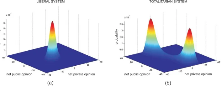
The critical behavior of a society moving from a lib-eral to a totalitarian political system can be evaluated when individuals are endowed with two separate opin-ions: a publicly pronounced and a privately held opinion for/against the ideology of the ruling party. The pub-lic and private opinions of an individual can be different when, for example, public dissent against the ruling ide-ology is a punishable offence. Along these lines, let us consider a fixed homogeneous group of 2L individuals who react in the same manner to a given situation. An individual simultaneously holds a public and a private opinion that each takes values 1/2 or−1/2 if it is for or against the ruling ideology, respectively. Let us denote byX1 the net public opinion, which corresponds to the
sum of the publicly held opinions of all 2L individuals. Likewise, let us denote byX2the net private opinion. We
are now dealing withN = 2 species interacting through the followingM = 4 reactions:
reaction 1 : X1+X2→2X1+X2
reaction 2 : X1+X2→X2
reaction 3 : X1+X2→X1+ 2X2
reaction 4 : X1+X2→X1.
(8)
The first two reactions model the influence of net pri-vate opinionX2on the net public opinionX1that results
in a single individual changing her public opinion in sup-port of (reaction 1) or against (reaction 2) the ruling
ideology. In this case, the net private opinion remains unchanged, whereas, the net public opinion is increased by one in reaction 1 [due to a value change from−1/2 (against) to 1/2 (for)] and decreased by one in reaction 2 [due to a value change from 1/2 (for) to−1/2 (against)]. Likewise, the subsequent two reactions model the influ-ence of net public opinionX1 on the net private
opin-ion X2 that results in a single individual changing her
private opinion in support of (reaction 3) or against (reac-tion 4) the ruling ideology. These reac(reac-tions are governed by the following propensity functions (Weidlich, 2006):
π1(xxx) =κ1(L−x1) exp(a1x1+a2x2) π2(xxx) =κ1(L+x1) exp(−a1x1−a2x2) π3(xxx) =κ2(L−x2) exp(a3x1)
π4(xxx) =κ2(L+x2) exp(−a3x1),
(9)
wherex1,x2 represent the net values of all publicly and
privately held opinions, respectively,κ1, κ2 >0 are two
specific probability rate constants associated with the four reactions, anda1 ≥0, a2 >0, a3 are three model
parameters. Note thatx1 andx2are integer-valued with
−L≤x1, x2≤L, where −Lrepresents total disapproval
andLrepresents total approval of the ruling ideology. Parametera1≥0 controls pressure inflicted on public
opinion due, for example, to oppression of this opinion by the ruling party (the value of this parameter is zero in the U.S. where free speech is protected, but strictly positive in countries where public dissidence has conse-quences). On the other hand, parametera2>0 controls
the influence of privately held beliefs on publicly stated opinions, whereas, parametera3controls how affirmative
(fora3>0) or dissident (fora3<0) the private opinion
is towards the ruling ideology. When the values ofa1and a3 vary, an abrupt change from a liberal to a totalitarian
political system can be observed (Weidlich, 2006). This critical social behavior predicted by the model is reminis-cent to the well-known phenomenon of phase transition in statistical mechanics and provides a crucial focus of study when dealing with opinion spreading in social net-works.
F. Neural networks
A discussion on reaction networks cannot be complete without mentioning biological neural networks. With 100 billion or more neurons in the human brain connected by 100-500 trillion synapses, there is no other reaction network that can compete in size and complexity.
There is a large body of literature surrounding the modeling and analysis of biological neural networks. As an example, we consider a Markovian reaction model for neural networks recently proposed by Benayoun et al.
(2010) that is intuitive enough for novices in neurobi-ology to comprehend and yet rich enough to be a viable candidate for understanding many features of this preem-inent reaction network. The model consists ofLneurons, with each neuron being in either a quiescent or an active
state. Let X2l−1 and X2l denote a quiescent or active
neuron l, respectively. We can assign the following two reactions to thel-th neuron in the network:
X2l−1+ X l06=l νl0lX2l0 → X2l+ X l06=l νl0lX2l0 X2l → X2l−1, (10)
where νij measures the synaptic weight between
neu-rons i and j, with a positive value indicating an exci-tatory synapsis and a negative value indicating an in-hibitory synapsis. Note that the first reaction models transition of the l-th neuron from the quiescent to the active state, which is assumed to be influenced by ap-propriately weighted active neurons X2l0, l0 6= l, in the network [see Eq. (11) below] that act as “catalysts.” On the other hand, the second reaction models transition of the neuron from the active to the quiescent state, which is assumed to occur constitutively. As a consequence, we obtain a reaction network with N = 2L species and
M = 2Lreactions.
We can describe this system by a 2L×1 state vector
xxxwith binary-valued 0/1 elements x2l−1, x2l indicating
the state of thel-th neuron (with 0 being quiescent and 1 being active). Due to the fact that a neuron must be either quiescent or active, the state variables must satisfy the mass conservation relationshipsx2l−1+x2l = 1, for
l= 1,2, . . . , L. It has been suggested by Benayounet al.
(2010) that the probability of thel-th neuron becoming active during an infinitesimally small time interval [t, t+
dt), given that the neuron is quiescent at time t, can be taken to bex2l−1[φl(xxx)>0] tanh[φl(xxx)]dt+o(dt), where
[a >0] is the Iverson bracket and φl is the net synaptic
input to thel-th neuron, given by
φl(xxx) =
X
l06=l
νl0lx2l0+hl, (11)
with hl being an external input to the neuron. The
termx2l−1ensures that the neuron becomes active within
[t, t+dt) only when it is quiescent at timet. As a con-sequence, the propensity of the first reaction in (10) will be given by
π2l−1(xxx) =x2l−1[φl(xxx)>0] tanh[φl(xxx)], (12)
and therefore depends on the synaptic inputs from neu-rons connected to thel-th neuron and any external input to that neuron. On the other hand, if we assume that the
l-th neuron decays from an active to a quiescent state at a constant rateγl, then the propensity of the second
re-action will be given by
π2l(xxx) =γlx2l, (13)
where the termx2lensures that the neuron becomes
in-active within [t, t+dt) only when it is active at timet.
G. Multi-agent networks
The study of multi-agent networks focuses on systems in which many intelligent agents, such as autonomous
ve-hicles that observe and act upon their environment, inter-act with each other to achieve a certain goal. To illustrate the fact that multi-agent systems can also be modeled as Markovian processes on reaction networks, we consider here a system comprised of L autonomous unmanned vehicles (AUVs) that can move over a two-dimensional bounded rectangular space in a discrete fashion (Xiet al., 2006). For simplicity, we assume that, at each step, an AUV located at a discrete point (i, j) in space can move towards one of four possible directions, namely east to point (i+ 1, j), west to point (i−1, j), north to point (i, j+ 1), or south to point (i, j−1). We want to develop a mathematical approach that can be used to describe vehicular motion so that the AUVs reach a spatial con-figurationxxxat steady-state with desired probabilityρ(xxx) which assigns high probability over configurations that maximize a given design objective and low or zero prob-ability over the remaining configurations. The construc-tion of such probability can be thought of as an inverse problem that can be solved using a statistical mechan-ics approach, as the one proposed by Cohn and Kumar (2009).
In the following, we employ two speciesX2l−1andX2l
whose populationsx2l−1 and x2l denote the position of
the l-th AUV on the two-dimensional rectangular grid. For example, if thel-th vehicle is located at point (i, j) on the grid, thenx2l−1 = i and x2l = j. We can now
characterize the motion of all AUVs in the multi-agent network under consideration byN = 2Lspecies interact-ing through the followinteract-ingM = 4Lreactions:
X2l−1+X2l+ X l06=l (X2l0−1+X2l0)→ 2X2l−1+X2l+ X l06=l (X2l0−1+X2l0) X2l−1+X2l+ X l06=l (X2l0−1+X2l0)→ X2l+ X l06=l (X2l0−1+X2l0) X2l−1+X2l+ X l06=l (X2l0−1+X2l0)→ X2l−1+ 2X2l+ X l06=l (X2l0−1+X2l0) X2l−1+X2l+ X l06=l (X2l0−1+X2l0)→ X2l−1+ X l06=l (X2l0−1+X2l0). (14)
The first two reactions model one-step motion of thel-th AUV towards east/west, whereas, the other two reactions model one-step motion towards north/south. Note that, when the first reaction occurs, the horizontal positioniof thel-th AUV is increased by one (transition fromX2l−1
to 2X2l−1), whereas its vertical position j remains
un-changed (transition fromX2l to itself). Moreover, this
is done by using the positions X2l0−1, X2l0, l0 6= l, of the remaining vehicles [see Eq. (16) below], which act as
“catalysts” of the reaction. Similar remarks apply for the other three reactions as well.
Let us now define the potential energy V(xxx) of the reaction system being in configurationxxxat steady-state by V(xxx) := −ln ρ(xxx) ρ(xxx0) , for xxx∈ D ∞, otherwise, (15)
where D is a set that contains all permissible vehicle configurations (e.g., xxx should not allow two vehicles to occupy the same grid position or positions occupied by obstacles, thus avoiding collisions or assignment of ve-hicles to grid positions outside the bounded rectangular region). Moreover,xxx0∈ Dis an appropriately chosen
ref-erence configuration of zero potential energy. Given that
XXX(t) =xxx, we can assume that, during the infinitesimally small time interval [t, t+dt), thel-th AUV can move one step towards east if two events take place: (a) during [t, t+dt), the AUV initiates motion with probability that is proportional todt, with proportionality factorκl, and
(b) given that the AUV initiates motion during [t, t+dt), it moves with probability exp{−V(xxx+sss4l−3)}, wheresssm
denotes them-th column of the net stoichiometric matrix of the reaction network given by (14). As a consequence, the AUV will be moving east with higher probability if the motion produces a larger reduction in potential en-ergy. Note that parameter κl controls the speed of the
l-th vehicle, with higher values of κl resulting in faster
motion.
By making similar assumptions for vehicle motion to-wards the other three directions, the dynamics on the reaction network given by (14) will be Markovian with propensity functions
πm(xxx) =κle−V(xxx+sssm), (16)
for m = 4l−3,4l−2,4l−1,4l, l = 1,2, . . . , L. Note thatsss4l−3,sss4l−2,sss4l−1 andsss4lequal e2l−1,−e2l−1,e2l,
and −e2l, respectively, whereem is the m-th column of
the 2L×2L identity matrix. It turns out that the re-sulting master equation governing the population pro-cessXXX(t) has a unique stationary distribution pX(xxx) := limt→∞pXXX(xxx;t), given by the Gibbs distribution
pX(xxx) =1 ζ e −V(xxx), (17) where ζ:=X x xx e−V(xxx) (18)
is the associated partition function. As a consequence of Eqs. (15), (17) and (18), we have that pX(xxx) =ρ(xxx). Therefore, the AUVs will asymptotically position them-selves in the two-dimensional space at locationsxxx with probabilityρ(xxx), as desired.
H. Evolutionary game theory
Game theory deals with mathematical models of con-flict and cooperation among intelligent and rational indi-viduals. Evolutionary game theory extends the paradigm of classical game theory by removing some stringent as-sumptions and by naturally incorporating the dynamic aspects of learning and experimentation into the prob-lem.
As an example of how evolutionary game theory can fit within the current context, suppose that a population ofLindividuals play with each other a game withN pos-sible strategiesX1, X2, . . . , XN. Let Xn(t) be the
num-ber of individuals playing strategyXn at time t. Here,
we consider a simple situation in which each individual competes with all other individuals. However, the frame-work presented in this paper is also capable of handling more general situations, such as those discussed by Sz-abo and Fath (2007). Given thatXXX(t) =xxx, letPn(xxx) be
the payoff to an individual playing the n-th strategy at timet. Based on the current payoff, this individual may decide at a random time to follow a new strategyXn0 in an attempt to improve his payoff. This can be modeled by the followingM =N(N−1) reactions:
Xn+Xn0+ X n006=n,n0 Xn00 → 2Xn0+ X n006=n,n0 Xn00, n0 6=n.
Note that, in this case, the number of individualsXn00 that follow strategies other thannandn0affect the tran-sition of an individual from strategynto strategyn0 [see Eq. (19) below] without changing their own strategies and, therefore, act as “catalysts.”
There are many alternative propensity functions that can be chosen to dictate when players will change their strategy, with each corresponding to different learning techniques or update rules (Szabo and Fath, 2007). A common choice however is given by the imitation rule of the Moran process (Moran, 1962):
π(xxx) =κxn L xn0Pn(xxx) P n00∈Nxn00Pn00(xxx) , (19)
whereκ >0 is a specific probability rate constant detail-ing how often individuals choose to update their strate-gies. The second term in Eq. (19) is the fraction of in-dividuals playing strategy Xn, whereas, the third term
is the fraction of the net payoff paid to individuals who play strategyXn0. These propensity functions have been originally developed to model natural selection and ge-netic drift in an asexually reproducing population of N
genetically distinct individuals, where each genotype rep-resents a strategy and the payoffs provide measures of reproductive fitness.
I. Petri nets
Petri nets have been extensively used to describe discrete-event distributed systems, a class of systems
that are of particular interest in computer science ap-plications (Diaz, 2009). A Petri net is a weighted, di-rected, bipartite graph, in which the nodes represent
placesandtransitions. Places model passive system com-ponents, whereas, transitions correspond to events that inter-convert places. Directed arcs join places to tran-sitions (connect places that can be converted during a transition) and transitions to places (connect a transi-tion with the corresponding products). Weights associ-ated with arcs indicate the multiplicity of the arc. Each place is associated withtokens, indicating the number of existing places. Whether or not a transition takes place is described by a rule, which may be deterministic or stochastic (Diaz, 2009; Haas, 2002), that depends on the number of tokens available in the places connecting to the transition by incoming arcs. The occurrence of a tran-sition results in removing a token from the input places and adding a token to the output places of the transition. The flow of tokens on a Petri net can be used to model the dynamics on a reaction network. As a matter of fact, a number of investigators (including Petri himself) have already proposed using Petri nets for modeling biochemi-cal reaction systems (Chaouiya, 2007; Goss and Peccoud, 1998; Heiner et al., 2008; Reddy et al., 1996). This approach however is very similar to traditional meth-ods for modeling biochemical reaction systems based on first-order differential equations or the chemical master equation, which have been extensively studied in the lit-erature (Gillespie, 1992; Heinrich and Schuster, 1996). In particular, Markovian Petri nets are identical to the Markovian reaction networks considered in this review, with the places playing the role of species and the transi-tions representing reactransi-tions. It is however important to carefully study the theory of stochastic Petri nets (Haas, 2002), since many results derived in that theory will likely prove very useful for the analysis of the Markovian reac-tion networks reviewed in this paper.
IV. SOLVING THE MASTER EQUATION
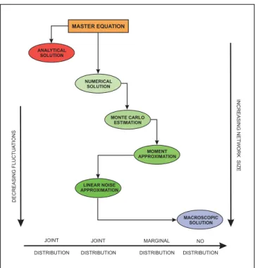
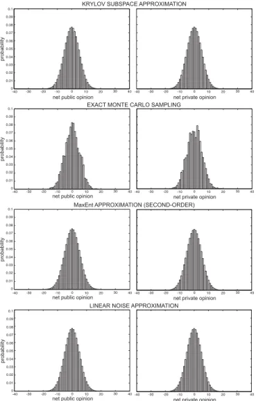
Although the algebraic form of the master equa-tions (4) and (5) is simple, solving these equaequa-tions [i.e., calculating the probabilitiespZZZ(zzz;t) andpXXX(xxx;t) at each timet >0] is a very difficult task in general. Many meth-ods have been proposed in the literature to address this problem, which can be grouped into the six general cate-gories depicted in Fig. 2. In the following, we discuss the most prominent techniques available to date. Whether a technique can be applied to a particular problem de-pends on the size and complexity of the reaction network at hand.
A. Exact analytical solution
Deriving exact analytical solutions for pZZZ(zzz;t) and
pXXX(xxx;t) is possible only in simple cases [e.g., see Darvey and Staff (1966); Gadgil et al.(2005); Gardiner (2010); Heuett and Qian (2006); Jahnke and Huisinga (2007); Laurenzi (2000); Leonard and Reichl (1990); McQuar-rie (1963); McQuarMcQuar-rieet al.(1964); Zhanget al.(2005)].
MASTER EQUATION ANALYTICAL SOLUTION NUMERICAL SOLUTION MONTE CARLO ESTIMATION LINEAR NOISE APPROXIMATION MACROSCOPIC SOLUTION
INCREASING NETWORK SIZE
JOINT JOINT MARGINAL NO
DECREASING FLUCTUA
TIONS
DISTRIBUTION DISTRIBUTION DISTRIBUTION DISTRIBUTION
MOMENT APPROXIMATION
FIG. 2 Six methods for solving the master equation. Some
methods can be used to approximate the joint probability
distributions of the DA and population processes while other
methods can only be used to approximatemarginal
distribu-tions. Analytical solutions can be obtained only in special cases. Numerical solutions are currently limited to small
re-action networks. Large networks require use of a moment
approximation scheme or adoption of linear noise approxima-tion method as opposed to Monte Carlo sampling. For large reaction networks, computing the macroscopic solution may be the only feasible choice. This solution however can only be trusted at low fluctuation levels.
For example, an analytical solution for the master equa-tion (5) can be derived in the case of alinearreaction net-work (i.e., a netnet-work with linear propensity functions). It has been shown by Gadgilet al.(2005) that, forclosed
linear reaction networks (i.e., linear reaction networks with fixed net population), the solution of the master equation (5) is a multinomial distribution, provided that the initial joint distribution is also multinomial. More-over, for open linear reaction networks (i.e., linear re-action networks with varying net population), the solu-tion of the master equasolu-tion (5) is a product Poisson dis-tribution, provided that the initial joint distribution is also product Poisson [see also Heuett and Qian (2006)]. These results are special cases of a more general result derived by Jahnke and Huisinga (2007) who have shown that the probability distributionpXXX(xxx;t) of the popula-tion process in a linear reacpopula-tion network with initial state
x
xx0 can be expressed as the convolution of multinomial
and product Poisson distributions with time-dependent parameters that evolve according to well-defined systems of first-order linear differential equations [see also (Zhang
B. Numerical solution
A substantial research effort has recently been focused on approximately solving the master equation (5) using numerical techniques. Although the methods developed so far show promise for addressing this problem, they are mostly limited to relatively small reaction networks. For this reason, we only provide a brief discussion here. The interested reader can find details in the references.
The master equation (5) can be expressed as a linear system ofcoupled first-order differential equations, given by
dppp(t)
dt =Pppp(t), (20)
for t > 0, where ppp(t) is a K×1 vector that contains the nonzero probabilities pXXX(xxx;t), xxx∈ X, of the popu-lation processXXX(t) andP is a largeK×K sparse ma-trix whose structure can be inferred directly from the master equation. For example, when the columns of the stoichiometric matrix S are all different from each other, the only nonzero elements of thei-th column ofP are theM off-diagonal elements, whose values are given byπm(xxxi), and the diagonal element, whose value is given
by −PM
m=1πm(xxxi), where M K is the number of
reactions. If we assume that the cardinality K of the state-spaceX is finite, then we can calculate the proba-bilitiespXXX(xxx;t) by solving Eq. (20), in which case
ppp(t) = exp(tP)ppp(0), (21) fort >0. This simple idea has led to a numerical tech-nique, proposed by Munsky and Khammash (2006), for approximately solving the master equation known as fi-nite state projection (FSP). This method requires an ap-propriate truncation of the state-space to determine the smallest possible set X and development of a compu-tationally feasible algorithm for calculating the matrix exponential in Eq. (21).
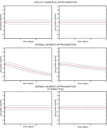
Although a number of methods are available for com-puting matrix exponentials [e.g., see Moler and van Loan (2003)], we briefly discuss here a popular tech-nique known as Krylov subspace approximation (KSA) method (Sidje, 1998; Sidje and Stewart, 1999). For a sufficiently small time step τ >0, this is the best avail-able method for approximating the vector ppp(t+τ) = exp(τP)ppp(t), when Pis a large and sparse matrix. This is done by using a polynomial series expansion of the form:
b p
pp(t+τ) =c0ppp(t) +c1τPppp(t) +· · ·+cK0−1(τP)
K0−1ppp(t),
where the coefficients c0, c1, . . . , cK0−1 are estimated by minimizing the least-squares error ||ppp(t + τ) − b
ppp(t + τ)||2
2. It turns out that the optimal K0
-th order polynomial approximation of ppp(t + τ) is a point in the K0-dimensional Krylov subspace K(t) =
spanppp(t), τPppp(t), . . . ,(τP)K0−1ppp(t) . This element can be approximated by
b p p
p(t+τ) :=||ppp(t)||2V(t) exp{τH(t)}eee1,
whereV(t) is a K×K0 matrix whose columns form an
orthonormal basis for the Krylov subspaceK(t) andH(t) is aK0×K0 Hessenberg matrix (upper triangular with
an extra subdiagonal), both computed by the well-known Arnoldi procedure (Sidje and Stewart, 1999). Finally,eee1
is the first column of theK0×K0identity matrix.
The KSA method reduces the problem of calculat-ing the exponential of a large and sparse K×K ma-trix P to the problem of calculating the exponential of the much smaller and denseK0×K0matrixH(K0K,
withK0= 30–50 being sufficient for many applications).
Computation of the reduced size problem can be done by standard methods, such as a Chebyshev or Pad´e approx-imation (Moler and van Loan, 2003; Sidje, 1998; Sidje and Stewart, 1999). Note that we can recursively esti-mate the solutionppp(t) in Eq. (21) at some timetj by
b p p
p(tj) = exp{(tj−tj−1)P}bppp(tj−1)
=||pbpp(tj−1)||2V(tj−1) exp{(tj−tj−1)H(tj−1)}eee1,
for j = 1,2, . . ., where bppp(0) = ppp(0) and 0 = t0 < t1 < t2<· · · is an increasing sequence of (not necessarily
uni-formly spaced) time points. These points are selected automatically, in conjunction with an appropriately de-signed error estimation procedure, to ensure stability and accuracy of the overall algorithm (Sidje, 1998).
Unfortunately, and for most realistic reaction net-works,Xcontains a very large number of states with non-negligible probability, thus making the practical imple-mentation of FSP difficult. This is a direct consequence of the fact thatX containsR1×R2×· · ·×RN distinct
el-ements, whereRnis an assumed maximum copy number
of the n-th species. A number of approaches have been proposed in the literature to address this problem (Deufl-hardet al., 2008; Heglandet al., 2007, 2008; Jahnke and Huisinga, 2008; MacNamara et al., 2008; Munsky and Khammash, 2007; Peleˇs et al., 2006; Wolf et al., 2010; Zhang et al., 2010a). Although some approaches per-form well, most are limited to small reaction networks. It turns out that the most difficult issue associated with these methods is solving the resulting system of differen-tial equations, which is usually prohibitively large.
We should point out here that another numerical ap-proach has been recently proposed in the literature that also attempts to address the previous problem (Jahnke, 2010; Jahnke and Udrescu, 2010). The method is based on representing the probability mass function of the pop-ulation process by an appropriately chosen wavelet de-composition scheme whose basis elements and the asso-ciated wavelet coefficients are being adaptively updated in time by solving a much smaller system of linear equa-tions. Although preliminary results indicate that the method works well, it is not clear at this point whether it can be efficiently used to evaluate population proba-bilities in reaction networks containing more than a few reactions and species.
The KSA method is based on several approximations, whose cumulative effect may appreciably affect its ac-curacy, numerical stability and computational efficiency.
These drawbacks can be addressed by solving the mas-ter equation (4) associated with the DA process, instead of Eq. (5). This leads to a recently developed numerical technique for solving the master equation known as im-plicit Euler(IE) method (Jenkinson and Goutsias, 2012). Similarly to the KSA technique, derivation of the IE method starts by expressing the master equation (4) as a linear system ofcoupledfirst-order differential equations, given by
dqqq(t)
dt =Qqqq(t),
fort >0, whereqqq(t) is aQ×1 vector that contains the nonzero probabilitiespZZZ(zzz;t),zzz∈ Z, of the DA process
ZZZ(t) and Qis a large Q×Qsparse matrix whose struc-ture can be inferred directly from the master equation (each column ofQcontainsM+ 1 nonzero elements that sum to zero, where M Qis the number of reactions). Ordering the elements inZ lexicographically results in a matrixQthat is lower triangular. As a consequence, and for a given time stepτ >0, we can use the implicit Eu-ler method for solving differential equations (Presset al., 2007) to estimateqqq(t) at discrete time points tj :=jτ,
j = 1,2, . . .. Thus, given an estimateqqqb(tj−1) ofqqq(tj−1),
an estimatebqqq(tj) ofqqq(tj) can be obtained by solving the
following system of linear equations: (I−τQ)bqqq(tj) =bqqq(tj−1),
whereIis theQ×Qidentity matrix. It has been shown by Jenkinson and Goutsias (2012) that this is possible for any value ofτ and can be efficiently done by a standard forward substitution scheme (Press et al., 2007). More-over, the resulting method is always stable, producing a valid probability vector at each iteration, whereas, its accuracy can be controlled by a single parameter, the step-size τ. Finally, we can use Eq. (6) to obtain an estimatebppp(t) of the probabilitiespXXX(xxx;t) frombqqq(t).
The IE method is computationally superior to KSA when the cardinality of the state-space Z is not appre-ciably larger than the cardinality of the state-space X. This however is not always possible, since the DAs are non-decreasing, whereas, the population numbers can ei-ther increase or decrease in a way that their values re-main within a fixed and bounded dore-main. As a conse-quence, this method can only be used when the number of reaction events are sufficiently constrained or remain small during a time interval of interest. The IE method has been used by Jenkinson and Goutsias (2012) to nu-merically approximate the solution of the SIR epidemic model discussed in Section III-C with remarkable success compared to the KSA method. In this case, the nullity of the stoichiometric matrixSis zero and, therefore, there is one-to-one correspondence betweenZZZ(t) andXXX(t), which implies that the state-spacesZ andX are isomorphic.
C. Monte Carlo estimation
Numerical approaches for solving the master equa-tion are not practical when the reacequa-tion network
con-tains many reactions and species. In this case, Monte Carlo sampling (Liu, 2001) can be used to evaluate the statistical behavior of the network. If, by simula-tion, we generate L sample trajectories {zzz(l)(t), t >0}, l = 1,2, . . . , L, of the DA process {ZZZ(t), t > 0}, then we can estimate the dynamics of its moments, such as of the means{µZZZ(m;t) := E[Zm(t)], t >0}and covariances
{cZZZ(m, m0;t) := cov[Zm(t), Zm0(t)], t >0}, by using the following Monte Carlo estimators:
b µZZZ(m;t) = 1 L L X l=1 z(ml)(t), bcZZZ(m, m 0;t) = 1 L−1 L X l=1 h zm(l)(t)−µbZZZ(m;t) i h zm(l)0(t)−bµZZZ(m 0;t)i.
Moreover, we can estimate the probability distribution
pZZZ(zzz;t) by using b pZZZ(zzz;t) = 1 L L X l=1 ∆(zzz(l)(t)−zzz),
for t > 0, where ∆(zzz) is the Kronecker delta function. Due to the simple relationship between the DA and pop-ulation processes given by Eq. (3), we can use similar estimators to approximate the dynamic evolution of the corresponding population statistics.
Unfortunately, to obtain sufficiently accurate Monte Carlo estimates, we need a large number of sample tra-jectories, which is computationally inefficient, especially when estimating high-order moments or probability dis-tributions.3 This problem can be addressed by
devel-oping computationally efficient approaches for sampling the master equation (4). In the following, we discuss a number of methods available in the literature.
1. Exact sampling
The simplest way to draw samples from the master equation (4) is by using the Gillespie algorithm (Gillespie, 1976, 1977, 1992). This method can generate a trajectory
{zzz(t), t >0} of the DA process by following two steps. First, given that the system is at statezzz(t) at timet, the timet+τof the next reaction to occur can be determined by drawing a sampleτfrom the exponential distribution:
et(τ) = ( X m∈M αm(zzz(t)) ) exp ( −τX m∈M αm(zzz(t)) ) , (22)
3When estimating probability distributions, the issue of efficiently
sampling low probability events is crucial and becomes the main bottleneck for deriving accurate and computationally efficient Monte Carlo estimators.