Volume 73: Graph Computation Models - Selected Revised Papers from GCM 2015

Volume 73 (2016)

Graph Computation Models

Selected Revised Papers from GCM 2015

Parallel Evaluation of Interaction Nets:

Case Studies and Experiments

Ian Mackie and Shinya Sato

20 pages

Guest Editors: Detlef Plump

Managing Editors: Tiziana Margaria, Julia Padberg, Gabriele Taentzer

Parallel Evaluation of Interaction Nets:

Case Studies and Experiments

Ian Mackie1and Shinya Sato2

1_{LIX, CNRS UMR 7161, ´Ecole Polytechnique, 91128 Palaiseau Cedex, France}

2_{University Education Center, Ibaraki University, 2-1-1 Bunkyo, Mito-shi,}

Ibaraki 310-8512, Japan

Abstract: Interaction nets are a particular kind of graph rewriting system that have many properties that make them useful for capturing sharing and parallelism. There have been a number of research efforts towards implementing interaction nets in parallel, and these have focused on the implementation technologies. In this paper we investigate a related question: when is an interaction net system suitable for par-allel evaluation? We observe that some nets cannot benefit from parpar-allelism (they are sequential) and some have the potential to be evaluated in a highly parallel way. This first investigation aims to highlight a number of issues, by presenting experi-mental evidence for a number of case studies. We hope this can be used to help pave the way to a wider use of this technology for parallel evaluation.

Keywords:Interaction nets, parallel evaluation, case studies

1

Introduction

Interaction nets are a model of computation based on a restricted form of graph rewriting: the rewrite rules must be between two nodes on the left-hand side, be local (not change any part of graph other than the two nodes), and there must be at most one rule for each pair of nodes. These constraints have no impact on the expressive power of interaction nets (they are Turing complete), but they offer a very useful feature: they are confluent by construction. The confluence property taken together with the locality constraint means that they lend themselves to parallel evaluation: all possible rewrites can be done in parallel.

case studies, and back up the work with experimental evidence using our own parallel evaluator developed to support this study.

The specific question that we propose in this paper is: when is a particular interaction net system well suited for parallel evaluation? More precisely, are some interaction nets “more parallel” than others? A question that naturally follows from this is: can we transform a net so that it is more suited for parallel evaluation? Once we have understood this, we can also ask the reverse question: can a net be made sequential? The purpose of this paper is to make a start to investigate these questions, and we begin with an empirical study of interaction systems to identify when they are suitable for parallel evaluation or not.

We take a number of typical examples (some common ones from the literature together with some new ones we developed for this paper) to see if they can benefit from parallel evaluation. In addition, we make some observations about how programs can be transformed so that parallelism is more useful. Using these examples, we give some heuristics for getting more parallelism out of an interaction net system. Our focus will be restricted to comparing different interaction net systems. Other platforms and programming languages supporting Parallel evaluation can be found in the literature (see for example [JS08,HS08]). We leave for a future study how useful interaction nets are in comparison to these alternative approaches.

The main contributions of the paper are:

1. Through examples and case studies we identify that some nets are sequential and some have potential for parallelism. We observe that it is also possible to transform a net to make it more parallel (and therefore by the reverse transform, more sequential).

2. We define an unbounded notion of parallel evaluation (all reductions possible are done in one step). We build an evaluator to measure this, and we test it with a number of examples.

3. Finally, we use our own parallel evaluator that not only gives some practical aspect of the case studies, but we can compare with extant parallel implementations.

This paper is the start of a research effort to understand better parallel evaluation of interaction nets, and to put them to practical use.

Structure. In the next section we recall the definition of interaction nets, and describe the notion of parallel evaluation that we are interested in. Through examples we motivate the ideas behind this work. In Section 3 we give a few small case studies to show how parallelism can have a significant impact on the evaluation of a net. In Section 4 we give some experimental results, and discuss these. Finally, we conclude in Section 5.

2

Background and Motivation

In the graphical rewriting system of interaction nets [Laf90], we have a setΣofsymbols, which

are the names of the nodes in our diagrams. Each symbol has an arityarthat determines the number ofauxiliary portsthat the node has. Ifar(α) =nforα ∈Σ, thenα hasn+1ports: n

α · · ·

x1 xn

Nodes are drawn variably as circles, triangles or squares. Anetbuilt onΣis an undirected graph

with nodes at the vertices. The edges of the net connect nodes together at the ports such that there is only one edge at every port. A port which is not connected is called afree port.

Two nodes(α,β)∈Σ×Σconnected via their principal ports form anactive pair, which is the

interaction net analogue of a redex. A rule((α,β) =⇒N)replaces the active pair(α,β)by the

netN. All the free ports are preserved during reduction, and there is at most one rule for each pair of agents. The following diagram illustrates the idea, whereNis any net built fromΣ.

α β

..

. ...

x1 xn

ym y1

=⇒ .._. N .._.

x₁ xn

ym y1

The most powerful property of this system is that it is one-step confluent: the order of rewrit-ing is not important, and all sequences of rewrites are of the same length (in fact they are just permutations). This has practical consequences: the diagrammatic transformations can be ap-plied in any order, or even in parallel, to give the correct answer. It is the parallelism aspect that we develop in this paper.

We define some notions of nets and evaluation. A net is called sequentialif there is at most one active pair that can be reduced at each step. We say that a net is evaluated sequentially if one active pair is reduced at each step. For our notion of parallel evaluation, we require that all active pairs in a net are reduced simultaneously, and then any redexes that were created are evaluated at the next step. We do not bound the number of active pairs that can be reduced in parallel. We remark that the number of parallel steps will always be less than or equal to the number of sequential steps (for a sequential net, the number of steps is the same for sequential and parallel evaluation).

As an example, consider unary numbers with addition. We represent the following term rewrit-ing system

add(Z,y) = y

add(S(x),y) = add(x,S(y))

as a system of nets with agentsZ,S,+:

Z S +

Z +

S +

S +

=⇒ =⇒

In this example, nets correspond to the terms in a very straightforward way. If we construct the net corresponding to the addition of two numbers, then we can observe that the addition of two numbers is sequential: at any time there is just one active pair, and reducing this active pair creates one more active pair, and so on. We call operations like thisbatchoperations. In terms of cost, reducing the net corresponding toadd(n,m)requiresn+1 interactions. If we consider the net corresponding to the termadd(add(m,n),p), then the system is still sequential, and the cost is now 2m+n+2. Using associativity of addition, the situation changes significantly. The net corresponding toadd(m,add(n,p))has sequential costm+1+n+1=m+n+2, and parallel costmax(m+1,n+1). Thus, using the associativity property of numbers, we obtain a system that is significantly more efficient sequentially, and moreover is able to benefit from parallel evaluation. The example becomes even more interesting if we change the rules of the rewrite system to an alternative version of addition:

add(Z,y) = y

add(S(x),y) = S(add(x,y))

The two interaction rules are now:

Z +

S +

+ S

=⇒ =⇒

Unlike the previous system, the termadd(add(m,n),p)already has scope for parallelism. We call operations like thisstream operations. The sequential cost is now 2m+n+2 and the parallel cost ism+n+2. But again, if we use associativity then we can do even better and achieve sequential costm+n+2 and parallel costmax(m+1,n+1)for the termadd(m,add(n,p)). These examples illustrate that some nets are sequential; some nets can use properties of the system (in this case associativity of addition) to get better sequential and parallel behaviours; and some systems can have modified rules that are more efficient, and also more appropriate to exploit parallelism. The next section gives examples where there is scope for parallelism in nets.

3

Case studies

Fibonacci. The Fibonacci function is a good example where many recursive calls generate a lot of possibilities for parallel evaluation. We build the interaction net system that corresponds to the term rewriting system:

fib 0 = fib 1 = 1

fib n = fib(n-1) + fib(n-2)

Using a direct encoding of this system together with addition defined previously, we can obtain an interaction system:

Fib Z ⇒ S Fib2

Z

Fib S ⇒

Fib2 Z ⇒ S

Z

Fib S

Fib

Dup

+

Fib2 S ⇒

S

Dup ⇒

S S

Dup Dup Z ⇒ Z Z

The following is an example of rewriting:

Fib

Fib S

Fib

Dup

+ S

Z S

S

Fib2

S

Z

→ →

Fib S

Fib

+

S

Z S

Z S

S

Z

→ã

fib 3 fib 1+ fib 2

0 1000 2000 3000 4000 5000 6000 7000 8000

0 2 4 6 8 10 12 14

steps

n

fib n (batch additive operation) sequential

parallel

0 1000 2000 3000 4000 5000 6000 7000 8000

0 2 4 6 8 10 12 14

steps

n

fib n (streaming additive operation) sequential

parallel

0 200 400 600 800 1000 1200

0 2 4 6 8 10 12 14

steps

n fib n (in parallel)

batch streaming

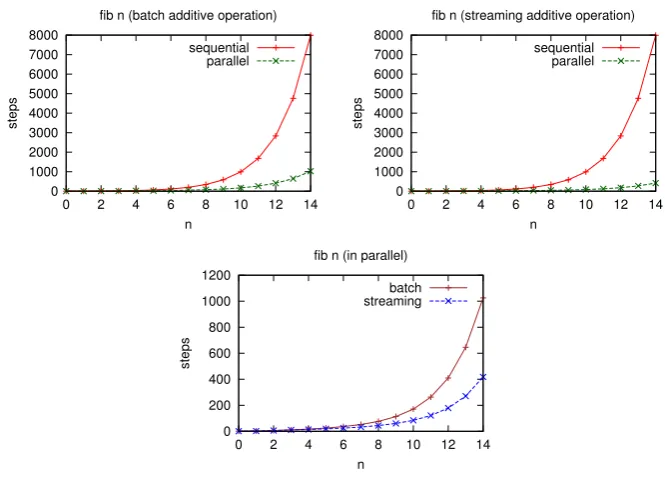
Figure 1: Comparing batch and streaming operations

elements of the given data and returns partial parts of the computational result immediately. The graphs in Figure1 show the number of interactions in each version, where we plot sequential steps against parallel steps to indicate the rate of growth of each one. Both graphs demonstrate that the sequential computation is exponential, while the parallel one is quadratic. We remark that, in the parallel execution, the number of steps with the streaming operation are less than a half of the numbers with the batch operation. This result is illustrated in the third graph in the figure.

By allowing attributes as labels of agents, we can include integer numbers in agents. In addi-tion, we can use conditional rewritings, preserving the one-step confluence, when these condi-tions on attributes are disjoint. In this case, the interaction net system representing the Fibonacci function is written as follows:

n ⇒

Fib

n=0

1

n ⇒

Fib

n=1

1

n ⇒

Fib

not(n=0) and

not(n=1) _Fib

n-1 Fib n-2 Add

n ⇒ Addn

(n)

m ⇒ n+m

Add

Addn (n)

0 500 1000 1500 2000 2500

0 2 4 6 8 10 12 14

steps

n fib n (integers)

sequential parallel

Ackermann. The Ackermann function is defined by three cases:

ack 0 n = n+1

ack m 0 = ack (m-1) 1

ack m n = ack (m-1) (ack m (n-1))

We can build the interaction net system on the unary natural numbers that corresponds to the term rewriting system as follows:

S

A ⇒ A2

A Z ⇒

y _{r x}

y _r

S

y _r r y

S

x

A2 Z ⇒

r

A

r

x

x

S

Z

Pred A2 S ⇒

y r

x

A

r A

y

Pred Dup

x

where the agentDupduplicatesSandZagents. The following is an example of rewriting:

S A

Z →

A2

→

A A

Pred Dup

ack 1 2

→ã

S

S

Z

S

S

Z S

Z

S

Z

S

Z

A S

Z A

S

Z

Z

(a) unary natural numbers

0 20000000 40000000 60000000 80000000 100000000 120000000 140000000

0 2 4 6 8 10

steps

n ack 3 n

sequential parallel

(b) integers

0 10000000 20000000 30000000 40000000 50000000 60000000 70000000 80000000 90000000

0 2 4 6 8 10

steps

n ack 3 n

sequential parallel

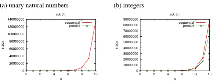
Figure 2: Benchmarks of the execution of Ackermann function in sequential and parallel

When we use numbers as attributes, the system can be written as:

1 ⇒

m₌0 m A

A2(m) ⇒

not(m=0) m

A

n ⇒

n=0

m_-1 A

n ⇒

not(n=0)

m_-1 A

m

n_-1 A

Addn

(1) A2(m)

A2(m)

Figure2shows the number of interactions in the cases of (a) unary natural numbers and (b) integer numbers, where we plot sequential steps against parallel steps to indicate the rate of growth of each one. Unfortunately, in Figure 2 (b), there is no significant difference in the sequential and the parallel execution, and thus there is no possibility of the improvement by parallel execution. This is because theAddnagent works as the batch operation, thus it waits for part of the result. For instance, after the last step in the following the computation stepack 2 1, the Addn(1) agent, which is the result of ack 0 (ack 1 0), waits for the computational result ofack 1 0. However, the computation ofA2should proceed because the result of the

Addn(1)will be more than 0.

A 2

1

→ã A2(1) A

A 0

1

0

→ A2(1) A

1

0 Addn

(1)

S A Z S S Z →ã A A S Z Z Z A2 S Z → A S Z Z A2 S Z S

Here, borrowing theSagent to denote numbers greater than 0, we change the rules, especially in the case ofack 0 n, by replacingAddnbySas follows:

1

A2(m) ⇒

not(m=0) m

A

n ⇒

n=0

m-1 A

n ⇒

not(n=0)

m-1 A

m

n-1 A

A2(m)

A2(m)

A2(m) ⇒ A m-1

m A

⇒ m=0 m

A S

Sum

(n) m ⇒ n+m

Sum

(n) ⇒

Sum (n+1)

S S

Thanks to the introduction of theSagent,A2can be processed without waiting for the result of

ack 1 0. This therefore gives a streaming operation:

A 2

1 →ã Sum

(0) A2(1) A

A 0

1

0

→ A2(1) A 1

0 S Sum (0) Sum (0)

In addition, the benchmark graph shows that the improved system is more efficient and more appropriate to exploit parallelism:

0 10000000 20000000 30000000 40000000 50000000 60000000 70000000

0 2 4 6 8 10

steps

n ack 3 n (integers, streaming)

sequential parallel 0 10000000 20000000 30000000 40000000 50000000 60000000 70000000

0 2 4 6 8 10

steps

n ack 3 n (integers, in parallel)

To summarise this section, a system can exploit parallelism by changing some batch operations into streaming ones. We leave as future work the criteria to determine when this transformation can benefit from parallelism.

Bubble sort. The simple sorting algorithm bubble sort can benefit from parallel evaluation in interaction nets. One version of this algorithm, written in Standard ML [MTHM97], is as follows:

fun bsortsub (x::x2::xs) =

if x > x2 then x2::(bsortsub (x::xs)) else x::(bsortsub(x2::xs)) | bsortsub x = x

fun bsort t =

let val s = bsortsub t

in if t=s then s else bsort s end;

Using a direct encoding of this program, we obtain the interaction system:

⇒

B_(x)

BS x

B₍x) x

BS Nil ⇒

⇒ Nil

⇒

⇒

B_(x)

B(x) y x B(y)

y B₍x)

Nil Nil

x ô y

not(x ô y)

EQn(x) _î

y

EQn(x) y

x = y

⇒ EQ

y

EQn(x)

y

not(x = y) ⇒

BS y

ï

EQ Nil ⇒ Ni

l

ï

EQ x ⇒ EQn(x)

where theδ andε agents are defined as a duplicator and an eraser:

î

î n

n î

⇒

⇒ Nil

n

Nil

Nil

ï Nil ⇒

ï n ⇒ _ï

For instance, a list[3,4,2]is sorted as follows:

BS 3 4 2 Nil _→

B₍3₎

EQn(3) _î 4 2 Nil

3

→ã

B(3)

EQn(3) 4 2 Nil

4 2 Nil

→

B(4)

EQn(3) 4 2 Nil

2 3

→ _EQn(3) 4 2 Nil

4 Nil

3

2

→ 4 2 Nil

4 Nil

EQ

3 2

→ã 2 Nil

4 Nil

BS

ï

B(3)

EQn(3) 2 4 Nil

2 4 Nil

→ã

3 2

→ã

2 4 Nil

4 Nil

ï

BS

→ã

B₍2₎

EQn(2) 3 4 Nil

3 4 _Nil

2 3

→ã Nil

4

Nil

EQ _→ã 2 3 4 Nil

This system shows that parallel bubble sorting is linear, whereas sequential evaluation is quadratic, as indicated in the graph below.

0 2000 4000 6000 8000 10000 12000 14000 16000

10 20 30 40 50 60 70

steps

n BS n (direct translation)

sequential parallel

However, it contains the equality test operation byEQandEQnto check whether the sorted list is the same as the given list. In comparison to the typical functional programming languages, interaction nets require copying and erasing of lists for the test that can cause inefficient compu-tation. Moreover, the sorting process is applied to the sorted list byBagain and again. Taking into account that theBmoves the maximum number in the given unsorted list into the head of the sorted list, we can obtain a more efficient system:

⇒

⇒ B(x)

BS x

B_(x) x

x BS _{Nil ⇒}

⇒

Nil

BS B(x)

BS M _⇒

⇒

⇒ B_(x)

B(x) y x B(y)

y B₍x)

Nil M _Nil

M M

x ô y

not(x ô y)

y

BS 3 4 2 _Nil

→ BS B₍3₎ 4 2 _Nil

→ BS 3 B₍4₎ 2 _{Nil →} BS 3 2 B₍4_{) Nil}

→ BS 3 2 M 4 Nil

→ BS B₍3₎ 2 M 4 Nil

→ BS 2 B₍3₎ M 4 Nil _→ BS 2 M 3 4 _Nil

M 3 4 _Nil

→ BS B(2) → BS M 2 3 4 Nil

Nil 4 3

→ 2

The system reduces the number of computational steps significantly, and gives the best expected behaviour as follows:

0 500 1000 1500 2000 2500 3000

10 20 30 40 50 60 70

steps

length BS n (improved)

sequential parallel

0 2000 4000 6000 8000 10000 12000 14000

0 50 100 150 200 250 300 350

steps

n BS n (in parallel)

direct improved

Map function. The map functionmaptakes a function f and a list[a1,a2, . . . ,an], returns a

list as follows:

map f [a₁,a₂, . . . ,an]=[f(a1),f(a2), . . . ,f(an)].

This function is well-known as a higher-order function in functional languages and also Google’s MapReduce [DG04]. Generally, we can build, for an agent f that has one auxiliary port:

f

the interaction net system such that an agentmapf works as the map function as follows:

mapf ⇒

f

n

n

mapf

opCons mapf Nil ⇒ Nil

where the agentopConsis defined as follows:

opCons n ⇒ n

mapFib 0 1 2 Nil

0 Fib

→

mapFib opCons

1 2 Nil

→ã

0 Fib

opCons Fib 1

opCons Fib 2

opCons

Nil

→ã 1 1 2 Nil

Here, for the benchmark, we just write MAPFib m n as the map application with the Fi-bonacci function and an-length list ofmsuch that[m,m,. . .,m], thusMAPFib 10 4means

map fib [10,10,10,10]. The following graph shows the benchmark of the execution

MAPFib 10 n in sequential and parallel evaluation:

0 1000 2000 3000 4000 5000 6000 7000

0 2 4 6 8 10 12 14 16 18

steps

n MAPFib 10 n

sequential parallel

This shows that both of the evaluations are linear, however the slope in the sequential evaluation is more steep than in the parallel evaluation. In the sequential evaluation each execution of

fib 10is accumulated, whereas in the parallel evaluation each is performed simultaneously. All these examples show the scope for harnessing parallelism from an empirical study: some systems do not benefit, whereas others allow quadratic computations be executed in linear par-allel complexity. However, these results give a flavour of the potential, and do not necessarily mean that they can be implemented like this in practice.

4

Discussion

Here we examine the potential of parallelism illustrated by the graphs in Section3, by using a multi-threaded parallel interpreter of interaction nets, calledInpla[Sat14], implemented with gcc 4.6.3 and the Posix-thread library. We compare the execution time of Inpla with other evaluators and interpreters. The programs were run on a Linux PC (2.4GHz, Core i7-3630QM, 16GB) and the execution time was measured using the UNIXtime command as the average of five executions.

First, for executions of pure interaction nets, we take INET [HMS09], amineLight [HMS10] and HINet [Kah15], and compare Inpla with those by using programs—the Fibonacci function (streaming additive operation) and the Ackermann function.

INET amLight HINet Inpla Inpla₁ Inpla₂ Inpla₃ Inpla₄ Inpla₅

fib 29 2.31 2.05 127.62 0.80 0.82 0.52 0.43 0.41 0.43

fib 30 3.82 3.40 609.64 1.25 1.26 0.76 0.63 0.61 0.60

ack 3 10 18.26 11.40 438.79 4.30 4.42 2.31 1.60 1.54 1.40

ack 3 11 66.79 46.30 1697.30 17.55 18.18 9.42 6.80 5.81 6.06

Table 1: The execution time in seconds of the pure interaction nets on interaction nets evaluators

1 2 3 4 5 6 7 8

1 2 3 4 5 6 7 8

S(n) (speedup)

n (threads) HINet

fib 29 fib 30 ack 3 10 ack 3 11

1 2 3 4 5 6 7 8

1 2 3 4 5 6 7 8

S(n) (speedup)

n (threads) Inpla

fib 29 fib 30 ack 3 10 ack 3 11

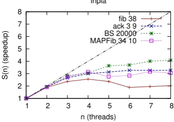
Figure 3: The speedup-ratio by multi-thread execution on HINet and Inpla

slowest since it evaluates a given net on an interpreter written by the Glasgow Haskell Com-piler (GHC) in comparison with INET that compiles it to source codes of the C programming language, and amineLight and Inpla that evaluate it on interpreters written by the C language. Inpla runs faster than INET since Inpla is a refined version of amineLight, which is the fastest interaction nets evaluator [HMS10].

In the table the subscript of Inpla gives the number of threads in the thread pool, for instance Inpla₂ means that it was executed by using two threads. Figure3illustrates the speedup-ratio

S(n) = T(1)

T(n) where T(i) is an execution time by i-threads. HINet uses Haskell parallel and

memory management framework, whereas Inpla manages these by simple mechanism for the sake of realising the fastest computation. Generally, we see similarity between these trends, although they are fluctuating.

SML Python Inpla Inpla₁ Inpla₂ Inpla₃ Inpla₄ Inpla₅

fib 34 0.12 2.09 1.67 1.50 0.80 0.70 0.68 0.82

fib 38 0.66 16.32 11.39 10.22 5.68 4.47 4.40 4.75

ack 3 6 0.03 0.05 0.02 0.03 0.02 0.02 0.02 0.02

ack 3 9 0.06 -1 0.69 0.72 0.38 0.27 0.24 0.24

BS 10000 1.64 6.71 2.11 2.25 1.17 0.87 0.76 0.68

BS 20000 8.38 30.35 8.38 8.93 4.57 3.64 2.98 2.49

MAPFib 34 5 0.49 9.89 8.92 8.09 4.55 3.21 2.54 2.73

MAPFib 34 10 0.94 19.77 17.81 17.23 9.28 6.44 5.22 5.38

1 _{RuntimeError: maximum recursion depth exceeded}

Table 2: The execution time in seconds on interpreters

1 2 3 4 5 6 7 8

1 2 3 4 5 6 7 8

S(n) (speedup)

n (threads) Inpla

fib 38 ack 3 9 BS 20000 MAPFib 34 10

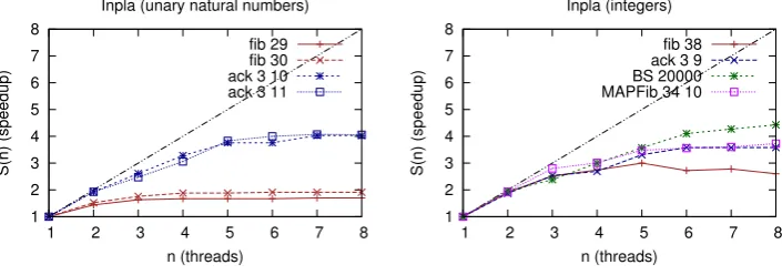
Figure 4: The speedup-ratio by multi-thread execution on Inpla

SML that performs computation by function calls and managing stacked arguments. In compar-ison with Python, Inpla computes those functions faster. The sort algorithm is a special case in that interaction nets are efficient to implement these algorithms. In the case of the map applica-tion, becausefib 34is applied 5 and 10 times, the execution time increases also about 5 and 10 times, respectively. Figure4illustrates the speedup-ratio by multi-thread execution on Inpla. Generally, since Core i7 processors have four cores, it tends to reach the peak with four or five execution threads.

Table 3 shows execution time in seconds on another Linux PC (4.2GHz, Core i7-6700K, 32GB), corresponding to Table1 and2. The speedup-ratio by multi-thread execution is illus-trated by Figure5. This processor also has four cores, hence it tends to reach the peak with four or five execution threads as well.

Next we analyse the results of the parallel execution in Inpla by using graphs in Section3, which show the trends of steps in parallel execution on the assumption of the unbounded re-sources. We may write “parallel(n)” in the following graphs to make explicit that Inplan is

used for the experiment.

Inpla Inpla₁ Inpla₂ Inpla₃ Inpla₄ Inpla₅ Inpla₆ Inpla₇ Inpla₈

fib 29 0.70 0.75 0.52 0.46 0.45 0.45 0.45 0.44 0.44

fib 30 1.04 1.11 0.73 0.63 0.59 0.59 0.58 0.58 0.58

ack 3 10 2.61 2.82 1.46 1.08 0.86 0.75 0.75 0.70 0.70

ack 3 11 10.62 11.44 5.92 4.64 3.74 2.99 2.86 2.81 2.82

fib 34 0.93 0.96 0.51 0.39 0.38 0.34 0.40 0.40 0.41

fib 38 6.28 6.51 3.41 2.58 2.38 2.17 2.39 2.34 2.50

ack 3 6 0.01 0.02 0.02 0.02 0.02 0.02 0.02 0.02 0.02

ack 3 9 0.39 0.43 0.23 0.17 0.16 0.13 0.12 0.12 0.12

BS 10000 1.33 1.58 0.79 0.55 0.51 0.46 0.39 0.38 0.37

BS 20000 5.30 6.11 3.11 2.57 2.04 1.71 1.49 1.43 1.38

MAPFib 34 5 4.74 4.90 2.54 1.87 1.64 1.40 1.49 1.48 1.46

MAPFib 34 10 9.48 9.78 5.06 3.49 3.25 2.81 2.75 2.72 2.62

Table 3: The execution time in seconds on another PC

1 2 3 4 5 6 7 8

1 2 3 4 5 6 7 8

S(n) (speedup)

n (threads) Inpla (unary natural numbers)

fib 29 fib 30 ack 3 10 ack 3 11

1 2 3 4 5 6 7 8

1 2 3 4 5 6 7 8

S(n) (speedup)

n (threads) Inpla (integers)

fib 38 ack 3 9 BS 20000 MAPFib 34 10

1.0 2.0 3.0 4.0 5.0 6.0 7.0 8.0

0 5 10 15 20 25 30

time (sec)

n

fib n (unary natural numbers, batch-add, Inpla)

sequential parallel(2) parallel(4)

1.0 2.0 3.0 4.0 5.0 6.0 7.0 8.0

0 5 10 15 20 25 30

time (sec)

n

fib n (unary natural numbers, streaming-add, Inpla)

sequential parallel(2) parallel(4)

0.0 1.0 2.0 3.0 4.0 5.0 6.0 7.0

0 5 10 15 20 25 30 35

time (sec)

n fib n (integers, Inpla)

sequential parallel(2) parallel(4)

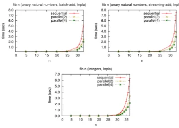
Figure 6: The execution time of Fibonacci function by Inpla

graphs on the assumption of unbounded resources (Figure 1). The increase rate of execution time in the parallel execution by Inpla gradually becomes close to, as we increase the number of threads, the trends of the parallel computation as given in Figure1.

We note that, in the computation of unary natural numbers, the execution of the streaming version is slower than the batch version as shown in the graph on the left side in Figure7. The graph on the right side shows the ratio of steps in the streaming version to steps in the batch version on the assumption of the unbounded resources. The ratio becomes around 0.4 according to increasingninfib n. This means that there is a limited benefit of the parallelism, even if we assume unbounded resources. In the real computation, the cost of parallel execution more affects the execution time in comparison to the benefit of the parallelism, and thus the streaming version becomes slower.

0.5 1.0 1.5 2.0 2.5 3.0

0 5 10 15 20 25 30

time (sec)

n

fib n (unary natural numbers, Inpla in parallel)

batch(4) stream(4)

0.0 0.2 0.4 0.6 0.8 1.0

0 5 10 15 20 25 30

ratio

n

streaming / batch (unbounded, in parallel)

Figure 7: Comparison between the batch and the streaming addition in parallel execution by Inpla

0.0 2.0 4.0 6.0 8.0 10.0 12.0 14.0 16.0 18.0

0 1 2 3 4 5 6 7 8 9 10 11

time (sec)

n

ack 3 n (unary natural numbers, Inpla)

sequential parallel(2) parallel(4)

0.0 5.0 10.0 15.0 20.0 25.0 30.0 35.0 40.0 45.0 50.0

0 1 2 3 4 5 6 7 8 9 10

time (sec)

n

ack 3 n (integers, batch, Inpla)

sequential parallel(2) parallel(4)

0.0 2.0 4.0 6.0 8.0 10.0 12.0

0 1 2 3 4 5 6 7 8 9 10 11

time (sec)

n

ack 3 n (integers, streaming, Inpla)

sequential parallel(2) parallel(4)

0.0 10.0 20.0 30.0 40.0 50.0 60.0

0 5000 10000 15000 20000

time (sec)

n BS n (direct, Inpla)

sequential parallel(2) parallel(4)

0.0 1.0 2.0 3.0 4.0 5.0 6.0 7.0 8.0 9.0

0 5000 10000 15000 20000

time (sec)

n BS n (improved, Inpla)

sequential parallel(2) parallel(4)

Figure 9: The execution time of Bubble sort by Inpla

0.0 5.0 10.0 15.0 20.0 25.0 30.0 35.0

0 2 4 6 8 10 12 14 16 18

time (sec)

n MAPFib 34 n (inpla)

sequential parallel(2) parallel(4)

Figure 10: The execution time of the map application by Inpla

Bubble sort.Figure9shows the execution time of the two programs for Bubble sort using Inpla. As anticipated by the graphs on the assumption of the unbounded resources, we see that the improved version performs best as expected.

Map function.Figure10shows the execution time of the map applicationMAPFib 34 nusing Inpla. As with Bubble sort, this algorithm performs well as we increase the number of threads.

5

Conclusion

may help in moving this work forward.

Bibliography

[DG04] J. Dean, S. Ghemawat. MapReduce: Simplified Data Processing on Large Clusters. In Brewer and Chen (eds.), 6th Symposium on Operating System Design and Im-plementation (OSDI 2004), San Francisco, California, USA, December 6-8, 2004. Pp. 137–150. USENIX Association, 2004.

http://www.usenix.org/events/osdi04/tech/dean.html

[HMS09] A. Hassan, I. Mackie, S. Sato. Compilation of Interaction Nets.Electr. Notes Theor. Comput. Sci.253(4):73–90, 2009.

[HMS10] A. Hassan, I. Mackie, S. Sato. A lightweight abstract machine for interaction nets.

ECEASST 29, 2010.

[HS08] M. Herlihy, N. Shavit. The Art of Multiprocessor Programming. Morgan-Kaufmann, 2008.

[Jir14] E. Jiresch. Towards a GPU-based implementation of interaction nets. In L¨owe and Winskel (eds.),DCM. EPTCS 143, pp. 41–53. 2014.

[JS08] S. P. Jones, S. Singh. A Tutorial on Parallel and Concurrent Programming in Haskell. InLecture Notes in Computer Science. Springer Verlag, 2008.

[Kah15] W. Kahl. A Simple Parallel Implementation of Interaction Nets in Haskell. In Lago and Harmer (eds.),Proceedings Tenth International Workshop on Developments in Computational Models, DCM 2014. EPTCS 179, pp. 33–47. 2015.

[Laf90] Y. Lafont. Interaction Nets. InProceedings of the 17th ACM Symposium on Princi-ples of Programming Languages (POPL’90). Pp. 95–108. ACM Press, 1990.

[MTHM97] R. Milner, M. Tofte, R. Harper, D. MacQueen.The Definition of Standard ML (Re-vised). MIT Press, 1997.

[Pin00] J. S. Pinto. Sequential and Concurrent Abstract Machines for Interaction Nets. In Tiuryn (ed.), Proceedings of Foundations of Software Science and Computation Structures (FOSSACS). Lecture Notes in Computer Science 1784, pp. 267–282. Springer-Verlag, 2000.

[RD11] G. van Rossum, F. L. Drake. The Python Language Reference Manual. Network Theory Ltd., 2011.