Scientific Big Data Visualization: a Coupled Tools Approach
Antoni Artigues1,2, Fernando M. Cucchietti1,3, Carlos Tripiana Montes1,4, David Vicente1,5, Hadrien Calmet1,6, Guillermo Mar´ın1,7, Guillaume Houzeaux1,8, Mariano Vazquez1,9
c
The Authors 2014. This paper is published with open access at SuperFri.org
We designed and implemented a parallel visualisation system for the analysis of large scale time-dependent particle type data. The particular challenge we address is how to analyse a high performance computation style dataset when a visual representation of the full set is not possible or useful, and one is only interested in finding and inspecting smaller subsets that fulfil certain complex criteria. We used Paraview as the user interface, which is a familiar tool for many HPC users, runs in parallel, and can be conveniently extended. We distributed the data in a super-computing environment using the Hadoop file system. On top of it, we run Hive or Impala, and implemented a connection between Paraview and them that allows us to launch programmable SQL queries in the database directly from within Paraview. The queries return a Paraview-native VTK object that fits directly into the Paraview pipeline. We find good scalability and response times. In the typical supercomputer environment (like the one we used for implementation) the queue and management system make it difficult to keep local data in between sessions, which im-poses a bottleneck in the data loading stage. This makes our system most useful when permanently installed on a dedicated cluster.
Introduction
High performance computer simulations can now routinely reach the peta-scale, producing up to tens or even hundreds of GB of data per single time step. The visualisation of such large data poses many challenges: from the practical details (e.g. visualisation must be done on site as the data is too large to move), to high level cognitive questions (e.g. how much and what part of the data is enough to reach meaningful conclusions.)
By far, the most time consuming operation in a large scale visualisation application is I/O. In a survey of visualisation performance on six supercomputers, Childs et. al. [1] showed that I/O time can be up to two orders of magnitude larger than calculation and render time. Re-cently, Mitchell, Ahrens and Wang [2] proposed a hybrid approach in which data was distributed across an HPC cluster using the Hadoop Distributed File System (HDFS), and used Kit-Wares ParaView as the user interface. The geometrical locality of data allowed to distribute the infor-mation such that each ParaView server had local access (through Hadoop) to the data needed for the distributed rendering. The performance increased linearly with the number of nodes used, following the effective bandwidth available to ParaView. However, this approach would have difficulty handling data that has time dependent geometry, or that requires parallel distri-bution along more than one variable. The example that motivated us was particle-like data from
1Barcelona Supercomputing Center, Department of Computer Applications on Science and Engineering, C/Gran Capita 2–4, Edifici Nexus I, Barcelona 08034 (Spain)
2[email protected] 3[email protected] 4[email protected] 5[email protected] 6[email protected] 7[email protected] 8[email protected]
biomechanical simulations, which move around during the simulation time, and that have phys-ical properties relevant for the visualisation but that do not correlate with the fixed geometrphys-ical information of the computational mesh.
We follow along the line of and propose a more flexible system, which allows to distribute the dataset simultaneously across many different variables, and that permits to interactively extract and visualise subsets that fulfil certain conditions. Specifically, we deploy the Apache Hive on top of Hadoop, and implement a set of plugins for ParaView users to interact directly through programmable actions. We have pre-programmed filters with typical questions like Where do the particles that ended up in a given region come from?, or find all particles and their trajectories that are of a given type and go through this region at a certain time. ParaView allows to configure the query regions or domains through the GUI, and the user does not need to enter any code. However, more complex questions can be configured only using the SQL-like language of Hive and integrated seamlessly in ParaView.
By using HDFS we are able to handle huge numbers of particles and time steps, and the coupling between ParaView and Hive allows us to interact, process, and visualise them in almost-real time. A simple geometrical distribution criteria would invariably produce unbalanced loads (e.g. at the initial time all particles are concentrated in the launch region). By not using HDFS directly but through Hive, our system allows us to distribute particles using criteria like physical properties or simply the number of particles. Another advantage of this setup is that the set of nodes running HDFS/Hive need not be the same used for Paraview. In fact, in principle they do not even need to be run on the same computer (although one can expect a latency cost in this configuration), similar to what can be seen in information visualisation software like Tableau [3]. In this paper we focus on outlining the architecture of the system as we implemented it for validation. We describe the separate tools we used, and what is required to couple them in a supercomputing environment. The dataset we used for testing is a simulation of the airflow through the human respiratory system performed by Alya [4] on the FERMI supercomputer, Italy. Although the set of filters we developed and tested were geared towards this biomechanical simulation, our system should be useful for all types of simulation that track particles moving in fluids or vector fields (e.g. supernova explosions or agent based modelling).
1. Background: The tools
1.1. Paraview
ParaView [5] is an open-source, multi-platform data analysis and visualization application. ParaView users can quickly build visualizations to analyze their data using qualitative and quan-titative techniques. The data exploration can be done interactively in 3D or programmatically using ParaView’s batch processing capabilities.
ParaView was developed to analyze extremely large datasets using distributed memory computing resources. It can be run on supercomputers to analyze datasets of petscale size as well as on laptops for smaller data. It has a client server architecture to facilitate remote visualization of datasets, and generates level of detail (LOD) models to maintain interactive frame rates for large datasets.
Paraview is developed in the C++ programming language, and it is possible to add new functionality to it through an extensive plugin mechanism that allows to:
• Add custom GUI components such as toolbar buttons to perform common tasks • Add new views in for display data
The plugins are based on the VTK library [6], an open-source system for 3D computer graphics, image processing and visualization. VTK consists of a C++ class library and several interpreted interface layers including Tcl/Tk, Java, and Python. With Paraview you can create a VTK filter library and integrate its functionallity into the Paraview data analisys pipeline with a custom GUI associated to this library.
1.2. Hadoop
Hadoop [7] is a complete open source software architecture designed to solve the problem of retrieving and analyzing large data sets with deep and computationally intensive operations, like clustering and targeting. Hadoop implements a distributed file system called HDFS (Hadoop Distributed File System) that is designed to be installed in a computer cluster. Each computer node on the cluster runs a Hadoop daemon (DataNode) that controls the local hard drives of the node as a part of the HDFS. Hadoop also runs a control daemon (NameNode) on one of the computer nodes, responsible for distributing and replicating files along the controlled hard drive nodes.
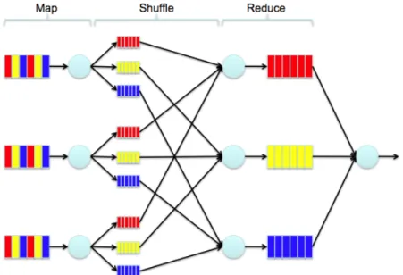
Hadoop allow users to execute MapReduce [8] jobs with the data stored in the HDFS. MapReduce is a functional-type programming model that allows to execute operations in parallel on the DataNodes, mapping the operations out to all of the Hadoop nodes and then reducing the results back into a single result set.
Figure 1. Example of MapReduce execution
1.3. Hive and other data warehouse software
In general, complex database query problems are easier to solve writing them in SQL-like notation than creating MapReduce jobs to solve them. Furthermore, connecting applications with ODBC database drivers are easier than connecting to a Hadoop cluster, as Hive provides an abstraction layer that facilitates using Hadoop as a data warehouse system.
Hive offers tools to improve the queries performance taking advantage of the Hadoop archi-tecture:
• Partitioning: Tables are linked to directories on HDFS with files in them. Without par-titioning, Hive reads all the data in the directory and applies the query filters on it. On the other hand, with partitioning Hive stores the data in different directories and allows to read a reduced number of directories when it applies a query.
• Bucketing: By organizing tables or partitions into buckets, one can decrease the response time of join operations: A join of two tables that are bucketed on the same columns (which include the join columns) can be efficiently implemented as a map-side join.
• Map-joins: Hive allows to load the entire table in memory to speed up the joins (this only works for tables that are smaller than the computer main memory size).
• Parallel Execution: Hive is capable of parallelizing the execution of complex SQL queries by default.
Impala [11] is another data base engine that works on top of Hadoop and in combination with Hive. It has its own query solver that replaces the MapReduce jobs generated by Hive. The Impala query solver works faster than Hive but requires more RAM memory in the nodes. We have performed local tests (in a workstation) with Impala, showing a remarkable improvement in the response times of the system compared to using only Hive. However, we have not been yet able to adapt Impala to our supercomputer queue system. We plan to continue working to adapt Impala to our infrastructure in a near future.
1.4. The physical problem
The physical problem that led us to develop our tools is the simulation of air flow through the human respiratory system. Of particular medical interest is the simulation of Lagrangian particles (transported by the fluid) that can represent medicine or pollutants in the air.
1.4.1. The Alya system
Alya is the BSC in-house HPC-based multi-physics simulation code. It is designed from scratch to simulate highly complex problems seamlessly adapted to run efficiently onto high-end parallel supercomputers. The target domain is engineering, with all its particular features: com-plex geometries and unstructured meshes, coupled multi-physics with exotic coupling schemes and Physical models, ill-posed problems, flexibility needs for rapidly including new models, etc. Since its conception in 2004, Alya has shown scaling behaviour in an increasing number of cores. Alya is one of the twelve codes of the PRACE unified European benchmark suite (http://www.prace-ri.eu/ueabs), and therefore complies with the highest HPC European stan-dards in terms of performance.
be found in [12–15]. The simulations were performed on the Blue Gene Q supercomputer Fermi (CINECA, Italy), through a regular PRACE access call [16].
1.4.2. Numerical solution
The particular simulation output we worked with consists of a unique CSV file, with each row specifying the properties for one particle: time step, position, velocity, type, family, etc. A typical simulation generates a 300 Gb file. While the size can clearly be reduced by adopting a binary format, the actual limitation was the previous software (in house developed) used to analyze the data which could only handle a few thousand particles and time steps. For analysis purposes, having a larger data set directly correlates with better statistics and finer results. In fig. 2 we show a 3D representation of a typical simulation.
Figure 2. Example of the simulation results CSV file
Experts in fluid dynamics and nasal inspiratory flows were interviewed in order to make a list of the most important questions they would like to see answered using the simulation results:
• What is the path followed by a certain particle? We want to view in the 3D environment the path that followed a single (selectable) particle from the first to the last simulation time step.
• How are particles mixed in a certain region? We have different particles types: oxygen, co2, drugs, and we want to know how they are mixed in a certain region. We also need a visual representation and a concentration percentage information.
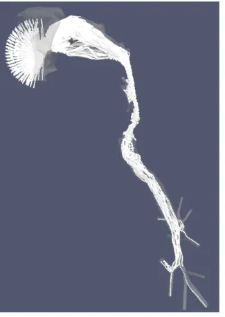
Figure 3. path followed by a certain particle
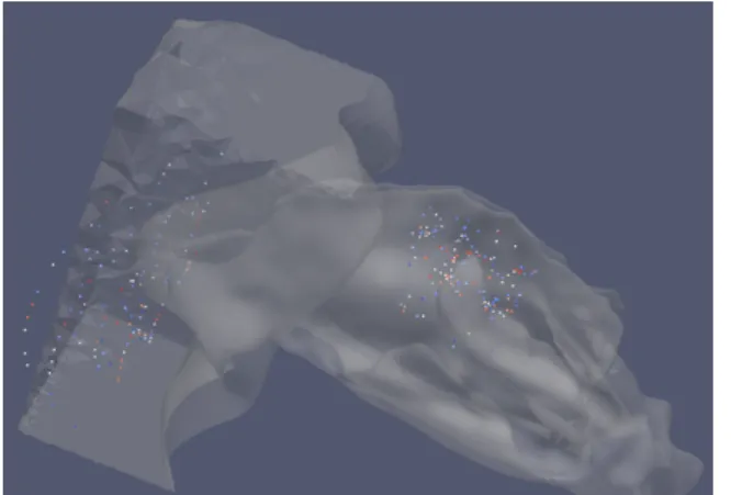
Figure 4. How are particles mixed in a certain region
Figure 5. Where do particles in certain region come from?
• What are the paths followed by particles that end up in a given region? We want to analyze how the particles arrived to their final positions in the smell region of the nose. With this analysis we can detect certain strange loops that happen in the particle paths, and we can try to improve the performance of the medical devices that supply the drugs. • How many particles go across a given section? We want to determine the throughput in
arbitrary nose regions.
• Show only the particles that have a particular velocity or other physical properties in a certain direction.
Figure 6. paths followed by the particles to a region
2. Requirements
The typical users of the application come from a biomedical background, are not experts in computational physics or high performance computing or IT. The application needs to be easy to use and avoid the complexity of the questions and its execution. Furthermore, it has to offer the results in a 3D, easy to understand, visual way.
The application has to offer tools to select precise 3D regions in a very accurate way. To carry out long analysis, the system has to answer the questions in real or almost real time, so that the user can work interactively with the application.
When the data is too big to be rendered the application has to filter the results selecting only a relevant number of particles.
Figure 7. Paraview user interface to analyze results
The application has to provide an easy and systematic way to add more pre-programmed questions.
• Use of batch queue systems: Because all the executions, including the Hadoop daemons, have to be launched through a queue job, no permanent Hadoop and Hive installation can be deployed in the supercomputer.
• Only ssh connections are allowed: We can not use the ODBC protocol to connect the user’s local computer with the Hadoop deployment on the supercomputer.
Due to this two restrictions, we must deploy the entire coupled tools and the full data set in the supercomputer each time that we need to analyze a simulation. Notice however that our system, as designed, can be easily installed in a permanent manner in a cluster without our supercomputer’s restrictions. Therefore, we do not consider them a crucial disadvantage of the architecture (it is a disadvantage of our available resources for implementation).
From the user’s point of view the steps to do the simulation analysis with our tools are: • Load the geometric mesh, in our case the respiratory system, into Paraview.
• Add a box source to the pipeline.
• Scale and translate the box to the desired 3D region. • Add a query plugin to the pipeline connected to the box.
• Select the desired query to execute from a list, for example: Obtain the particle’s paths that are in the region and goes from outside to inside the nose.
• Click apply and obtain the results, in about 15 seconds depending on the query, on the 3D Paraview panel.
3. Architecture
3.1. Structure
In this section we describe how we coupled the different tools in order to solve the require-ments described above.
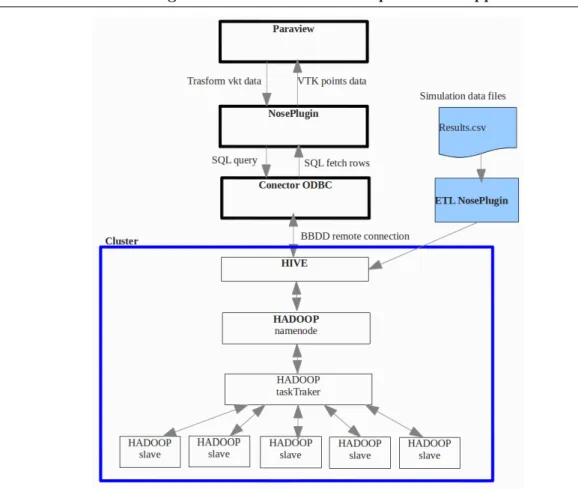
As is shown in fig. 8, the main components of the structure are: • Paraview: User interacts with Paraview to analyze the results
• NosePlugin: We have developed this Paraview plugin that allows users to query the sim-ulation data.
• ODBC connector: Connects the NosePlugin with the data base.
• ETL NosePlugin: A script that loads all the simulations results into the database. • Hive: The relational and distributed database engine in charge of executing SQL queries. • Hadoop: The distributed file system used by Hive to execute the SQL questions in parallel
through map-reduce jobs.
• Cluster: Hadoop works on top of a computer cluster, it needs a minimum of two nodes in order to run correctly.
3.2. Workflow
In this section we explain what are the steps required to solve a question about the simulation results.
Figure 8. Coupled tools structure
Notice that the following first two steps are special and must be repeated every time the architecture is used only in a queue system that does not allow permament installations of software. In a dedicated cluster setup they are executed once at deployment and are not a crucial part of our system.
3.2.1. Deploy services
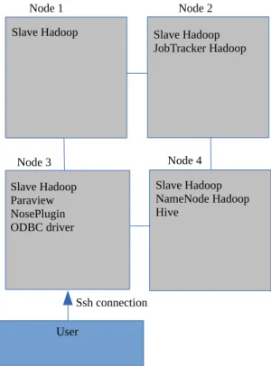
The first step is to deploy the Hadoop and Hive infrastructure in a subset of a supercomputer nodes, see fig. 9. The infrastructureJob:
• Allocates the required nodes and gets their IP addresses.
• Creates the required Hadoop folders in each of the nodes local hard drives.
• Creates the Hadoop configuration files to run Hadoop correctly in the allocated nodes. • Configures the ODBC driver with the correct IP address
• Starts the Hadoop and Hive daemons on the nodes • Starts the ETL NosePlugin Python script.
The deployment step requires a minimum of two nodes in order to work properly and three nodes to have data replication.
3.2.2. Load data
The script executes these steps:
1. Prepare data: Checks the data file integrity and cleans unnecessary data.
2. Create database tables: Creates all the relational tables necessary to store the simulation results(see fig. 10)
3. Iterates over the CSV simulation results file (a) Gets next n lines from the file.
(b) Generates a temporal file with these n lines.
(c) Loads this temporal file data into a temporal relational table with the LOAD DATA command.
(d) Loads the data into the final tables with a list of ”INSERT SELECT” SQL statements. In order to load big data files to the system we have done these optimizations:
• Adjust the partitions number to the data size
• Adapt Hadoop mapred-site.xml configuration to the supercomputer. • Check SQL exceptions and try one more time when errors happen. • Partition the main CSV file in slices
• Open and close connection with the database each time.
Slave Hadoop Paraview NosePlugin ODBC driver
User
Ssh connection Slave Hadoop
Node 1 Node 2
Node 3
Slave Hadoop NameNode Hadoop Hive
Node 4 Slave Hadoop JobTracker Hadoop
Figure 9. Coupled tools deployment in the Minotauro Supercomputer with 4 nodes
3.2.3. Start Paraview and NosePlugin
3.2.4. Prepare Paraview to ask questions to the system
At this point the user can interact with the Paraview instance. The first step is to load the geometric nose mesh into Paraview. This mesh has to be small (meaning that it can be stored in the user’s local file system). The next step is to add and position a box into the pipeline. Finally the user has to load the nosePlugin attached to the box.
3.3. Asking questions to the system
The user now can select a question from the nosePlugin GUI and click ”apply”. In that moment:
1. the nosePlugin receives the box position thought a VTK object data and the question to be asked to the data base in a string field.
2. The nosePlugin creates the SQL query and sends it to the data base through the ODBC Connector.
3. The Hadoop and Hive cluster is in charge of solving the query in real time.
4. The nosePlugin receives from the data base the SQL fetched rows corresponding to the answer.
5. The nosePlugin transforms the response into a VTK object and sends it to Paraview
4. Testing and validation
4.1. Validation
In order to do a basic test and validation we ran a small simulation that contains 2256 particles and 867 timesteps. This test case took only 184MB of disk storage. We installed the entire infrastructure in a standalone laptop and we ran the entire workflow on this machine.
We asked the system for the particles list in a well known region and time step, and we compared the obtained results with the expected response to validate the entire architecture.
4.2. Minotauro implementation
We deployed the architecture in the Minotauro supercomputer [18]. Minotauro has 126 compute nodes, each node has 12 cores, 24 GB of RAM memory, 12MB of cache memory and 250 GB flash local disk storage. Each also has two NVIDIA M2090 cards, each one with 512 CUDA Cores.
The HDFS was installed in the local flash disk of each node, the total available storage for Hadoop is 178.83 GB per node.
We developed a bash script in order to deploy the architecture in Minotauro each time that we needed to analyze results. The script is launched in the SLURM Minotauro queue system and installs Hadoop and Hive dinamically depending on the resources requested by the user and the nodes caught by the queue system.
4.3. Tests and scalability
4.3.1. Scalability test — number of nodes
The first scalability test consisted of:
1. Loading the 60GB file in 4, 8 and 16 nodes in Minotauro
2. Obtaining the particles that are inside a cube with the corresponding SQL query. 3. Measuring the time taken to resolve the query.
Figure 10.Tables database structure
Figure 11.Scalability for the 60GB results file
Table 1. Scalability results for 60GB
Nodes Response time Speed up Ideal
2 185.24 s 1 1
4 80.97 s 2.27 2
8 46.83 s 3.95 4
16 34.87 s 5.31 8
2.2878374314 3.9555077263 5.3116754452
4.3.2. Scalability test — size of the dataset
The second scalability tests consisted of:
1. Loading the 60GB and 120GB files in 8 Minotauro nodes.
2. Obtaining the particles that are inside a cube with the corresponding SQL query for both file sizes.
3. Measuring the time taken to resolve the query on each file. The times we measured are:
Nodes 60GB file 120GB file 8 46.83 s 50.97 s
which suggests that our system scales well with the size of the dataset. The expected time for 120GB was 93.66 seconds, but we obtained 50.97 seconds. This confirms that the scalability is better than the expected before reaching the ideal number of nodes. For example, with the 60GB file from 2 two 8 nodes the performances are better than the expected, but for 16 nodes the response time is below ideal.
4.3.3. Optimization test
The optimization test is based on quantifying the speed-up obtained when we apply different Hive optimizations to the queries:
• Star data base schema • Hive map joins
• Hive partitioning in time dimension • Hive partitioning in space dimensions
We loaded a 15GB results file into 4 Minotauro nodes, we obtained the particles that are inside a cube with optimized and not-optimized queries respectively. The response time, in seconds, for both queries:
Nodes not optimized optimized
4 430.19 s 78.81 s
With Hive optimizations we obtained a speed up of 5.4x in our queries, emphasizing the fact that database optimization is a crucial aspect in all systems based on distributed technologies.
4.3.4. Impala test
In this test we compared the performance between Hive and Impala using a 184MB dataset. Because we could not install Impala in our supercomputers, we used a Cloudera Virtual Machine with Impala, Hive and Hadoop preinstalled on it. We obtained the particles that are inside a cube with the corresponding SQL query for both systems: Impala and Hive. The response times in seconds were:
Impala Hive 0.712 15.043
4.4. User feedback
positive feedback, in the sense that our tool has allowed them to improve their workflow con-siderably and will allow them to refine their observations (by increasing the number of particles they simulate). Users also point out the ease of designing new queries into the system, which they feel as a natural extension of Paraview capabilitites. They have identified two problems: the setting up stage is too long and inconvenient, and the response time, although short, is still away from real-time.
5. Conclusions
We have designed and implemented a system for the visualization and analysis of particle-type large sets of data using a coupled tools approach. Through testing we verified that the efficiency of the system scales well with the amount of resources used (e.g. number of compute nodes), meaning that it is a viable approach for larger (peta-scale) datasets where the tools we used have already been tested. Our test implementation would not scale up to peta-sized databases because of the constrains imposed by the supercomputer queue system (which would require days just to load the data set), but in a normal cluster environment with a permanent Hadoop and Hive installation this would not be a problem. Although the set of filters we devel-oped and tested were geared towards our particular biomechanical simulation study case, our system should be useful for all types of simulation that track particles moving in fluids or vector fields (e.g. supernova explosions or agent based modelling). The problems detected by users will be resolved in the near future with a production version of our system installed permanently in a small cluster, where we will also be able to install and use Impala to improve the responsiveness of the queries. In the future we will investigate the parametrization of the trajectories in the data set into e.g. Bezier curves, thus moving the complexity of the data queries into computational complexity.
This work was partially supported by the Spanish Severo Ochoa Program, grant SEV-2011-00067. We acknowledge PRACE for awarding us access to the resource FERMI based in Italy at CINECA.
This paper is distributed under the terms of the Creative Commons Attribution-Non Com-mercial 3.0 License which permits non-comCom-mercial use, reproduction and distribution of the work without further permission provided the original work is properly cited.
References
1. H. Childs, E. Brugger, K. Bonnell, J. Meredith, M. Miller, B. Whitlock, and N. Maxi. A contract based system for large data visualization. In Visualization, 2005. VIS 05. IEEE, 2005.
2. Christopher Mitchell, James Ahrens, and Jun Wang. Visio: Enabling interactive visualiza-tion of ultra-scale, time series data via high-bandwidth distributed i/o systems. In Parallel & Distributed Processing Symposium (IPDPS), 2011 IEEE International, 2011.
4. Alya system - large scale computational mechanics. http://www.bsc.es/
computer-applications/alya-system.
5. Paraview software. http://www.paraview.org. Paraview is developed by Kitware company.
http://www.kitware.com.
6. VTK api. http://www.vtk.org. VTK is developed by Kitware company. http://www. kitware.com.
7. Hadoop. http://hadoop.apache.org/.
8. Yang Hung-Chih, Ali Dasdan, Hsiao Ruey-Lung, and D. Stott Parker. Map-reduce-merge simplified relational data processing on large clusters. In Proc. of ACM SIGMOD, 2007.
9. Hive database engine. http://hive.apache.org/.
10. Information technology database languages sql. http://www.iso.org/iso/iso_
catalogue/catalogue_tc/catalogue_detail.htm?csnumber=53681. ISO/IEC
9075-1:2011 standard.
11. Impala database engine. http://impala.io. Impala is developed by Cloudera company.
http://www.cloudera.com.
12. G. Houzeaux, R. Aubry, and M. V´azquez. Extension of fractional step techniques for in-compressible flows: The preconditioned orthomin(1) for the pressure schur complement.
Computers & Fluids, 44:297–313, 2011.
13. G. Houzeaux, R. de la Cruz, H. Owen, and M. V´azquez. Parallel uniform mesh multiplication applied to a navier-stokes solver. Computers & Fluids, 80:142–151, 7 2013.
14. G. Houzeaux, H. Owen, B. Eguzkitza, C. Samaniego, R. de la Cruz, H. Calmet, M. V´azquez, and M. ´Avila. Developments in Parallel, Distributed, Grid and Cloud Computing for Engi-neering, volume 31 of Computational Science, Engineering and Technology Series, chapter Chapter 8: A Parallel Incompressible Navier-Stokes Solver: Implementation Issues, pages 171–201. Saxe-Coburg Publications, b.h.v. topping and p. iv´anyi (Editor) edition, 2013.
15. M. V´azquez, G. Houzeaux, S. Koric, A. Artigues, J. Aguado-Sierra, R. Ar´ıs, D. Mira, H. Calmet, F. Cucchietti, H. Owen, A. Taha, and J.M. Cela. Alya: Towards exascale for engineering simulation codes. arXiv.org, 2014.
16. G. Houzeaux. Numerical simulation of air flow in the human large airways. PRACE 4th regular call. 20m core hours on tier-0, Fermi (I)., 2012.
17. Supercomputer description. http://en.wikipedia.org/wiki/Supercomputer.
18. Minotauro - nvidia gpu cluster. http://www.bsc.es/marenostrum-support-services/