The estimation of flood quantiles in ungauged sites using teaching-learning based optimization and artificial bee colony algorithms

(1)

Sharif University of Technology

Scientia Iranica

Transactions A: Civil Engineering http://scientiairanica.sharif.edu

The estimation of ood quantiles in ungauged sites

using teaching-learning based optimization and

articial bee colony algorithms

T. Anlan

_{, E. Uzlu, M. Kankal, and}

_{O. Yuksek}

Department of Civil Engineering, Faculty of Engineering, Karadeniz Technical University, 61080 Trabzon, Turkey. Received 29 February 2016; accepted 12 November 2016

KEYWORDS Regional ood frequency analysis; L-moments; Teaching-learning based optimization; Articial bee colony algorithm;

Turkey.

Abstract. In this study, a Regional Flood Frequency Analysis (RFFA) was applied to 33 stream gauging stations in the Eastern Black Sea Basin, Turkey. Homogeneity of the region was determined by discordancy (Di) and heterogeneity measures (Hi) based

on L-moments. Generalized extreme-value, lognormal, Pearson type III, and generalized logistic distributions were tted to the ood data of the homogeneous region. Based on the appropriate distribution for the region, ood quantiles were estimated for return periods of T = 5; 10; 25; 50; 100, and 500 years. A non-linear regression model was then developed to determine the relationship between ood discharges and meteorological and hydrological characteristics of the catchment. In order to compare regression analysis with other models, Articial Bee Colony algorithm (ABC) and Teaching-Learning Based Optimization (TLBO) models were developed. The equations were obtained using the ABC and TLBO algorithms to estimate ood discharges for dierent return periods. The analysis showed that the TLBO and ABC results were superior to the regression analysis. Error values indicated that the TLBO method yielded better results for the estimation of ood quantiles for dierent independent variables.

1. Introduction

Reliable estimation of ood discharges has great im-portance in the planning, design, and management of hydraulic structures. Regional Flood Frequency Anal-ysis (RFFA) enables estimation of ood magnitudes in dierent return periods at any stream location where stream ow data are quite limited or completely absent. Thus, RFFA is frequently used to obtain design ood estimates.

*. Corresponding author. Tel.: +90 462 3772654; Fax: +90 462 3772606

E-mail addresses: [email protected] (T. Anlan); [email protected] (E. Uzlu); [email protected] (M. Kankal); [email protected] ( O. Yuksek).

doi: 10.24200/sci.2017.4185

Identication of homogeneous regions, selection of appropriate regional frequency distribution, and estimation of ood quantiles at sites of interest are the basic concepts of RFFA. Many RFFA methods have been developed up to now. Some of the most commonly adopted RFFA methods in practice include (i) the rational method, (ii) index ood procedures with prob-ability weighted moments and L-moments, and (iii) regression and articial intelligence based methods [1]. As an example of rational method, Jiapeng et al. [2] proposed formulas that are modications of the tradi-tional ratradi-tional formula and able to calculate the ood design peak discharges. The use of the index ood procedure started with Wallis [3], who used it in con-junction with probability weighted moments and the Wakeby (WAK) distribution as a method of estimating quantiles in the frequency distribution. Probability

(2)

weighted moments were found to perform well for other distributions, but were hard to interpret [4]. Hosking [5] found that certain linear combinations of probability weighted moments, which he called the \L-moments", have some theoretical advantages over conventional moments of being able to characterize wider range of distributions.

So far, a variety of L-moments based methods have been extensively investigated in RFFA across the world to obtain more reliable estimates. Rao et al. [6] analyzed maximum ow data from 93 sites in the Wabash River, USA, using L-moments, and concluded that Generalized-Extreme Value (GEV) distribution appeared to be more robust to the region. Parida et al. [7] performed a regional ood frequency analysis on Mahi-Sabarmati basin in India using the L-moments and index ood procedure. They modeled oods in the region using the Lognormal (LN) distribution as the appropriate distribution. Adamowski [8] studied prob-ability density functions for oods in the Provinces of Ontario and Quebec, Canada. In Turkey, Haktanir [9], Sorman and Okur [10], Atiem and Harmancioglu [11], Saf [12], and Bayazit and Onoz [13] carried out L-moments based RFFA. In recent years, Seckin et al. (2011) showed that GEV and WAK distributions, whose parameters are computed by the L-moments method, are adequate in predicting quantile estimates in Turkey. Seckin et al. [14] then enhanced their L-moments based study with articial intelligence tech-niques to predict ood peaks of various return periods at ungauged sites in that basin in Turkey. It was con-cluded that the Multi-Layer Perceptrons (MLP) model is observed to ensure estimates close to the L-moments approach. Aydogan et al. [15] applied a RFFA to Coruh Basin by L-moments method in Turkey. They estimated ood quantiles and compared them with those estimated previously by an at-site frequency analysis (Gumbel distribution) on the basin master plan for four large dams in the Coruh Basin. Frat et al. [16] also calculated ood discharges for Turkey using distribution function parameters and observed higher error values with the increase of recurrence period.

The spatial variations in ow statistics are closely related with the variations in regional physiographical and meteorological factors. Quantile Regression (QR) models are often used to make estimates of ow statistics for ungauged sites and their relationships between catchment properties [17,18]. Ouarda et al. [19] applied the Canonical Correlation Analysis (CCA) technique to a dataset of 106 stations from the province of Ontario, Canada, and presented its usefulness in RFFA. Jingyi and Hall [20] performed Residuals method, Ward's cluster method, the fuzzy c-means method, and Kohonen neural network on 86 sites in the Gan River Basin and the Ming River Basin in China to identify homogeneous regions based on

site characteristics; they also examined the discordancy and homogeneity of the groups by L-moments of the distribution of annual oods. Reis et al. [21] introduced a Bayesian analysis of the Generalized Least Squares (GLS) model, which provides measures of the model error variance that are more accurate. Many studies with regression-based techniques [22-31] have been used to describe quantitative relationships between independent and dependent variables.

As an alternative to these methods, articial intelligence methods can be applied to RFFA by com-bining several methods [32]. Dawson et al. [33] used Articial Neural Networks (ANN) model for RFFA, and concluded that ANN provided more accurate ood quantile estimates than the traditional regression techniques. Shu and Ouarda [34] integrated CCA and ANN for ood quantile estimation at ungauged sites in Quebec, Canada. They concluded that the proposed CCA-based ANN models presented better performance than the original ANN models. Shu and Ouarda [35] provided a general framework named as Adaptive Neuro-Fuzzy Inference System (ANFIS) with combining two techniques, i.e. ANN and fuzzy systems. Their study revealed that the ANFIS model provided an integrated mechanism for identifying the hydrological regions and ood estimates with non-linear modeling capability. Aziz et al. [36] compared the performances of the ANN-based RFFA model with classical regression techniques, and indicated that ANN presented the best performing RFFA model. Seckin et al. [14] applied ANN models to compare them with multiple regression ones. They found that the performance of the ANN-MLP model is superior to the others.

With the increase in the application of articial intelligence techniques in hydrology, optimization tech-niques have also been frequently used in this area in recent years. Chau [37] used Particle Swarm Opti-mization training algorithm (PSO) to predict water levels in Shing Mun River of Hong Kong with dierent lead times based on the upstream gauging stations or stage/time history at the specic station. It was shown that the PSO technique could act as an alternative training algorithm for ANNs. Jiong-feng and Wan-chang [38] applied Genetic Algorithm model (GA) to the daily rainfall-runo simulations, and indicated that the proposed approach was feasible and of high computational eciency and could be transferred to model parameter calibrations for conceptual hydrolog-ical models in the similar categories. Jun et al. [39] proposed an Ant Colony Optimization-based (ACO) support vector machine algorithm SVM model (ACO-SVM) to optimize the parameters using an ACO random-seeking strategy. It was concluded that ACO-SVM is much more ecient in global optimization and its forecasting accuracy is better than that of the

(3)

con-ventional parameter-choosing method. Kisi et al. [40] investigated Articial Bee Colony algorithm (ABC) for modeling discharge-suspended sediment relationship and compared the model with neural dierential evolu-tion, adaptive neuro-fuzzy, neural networks, and rating curve models. They concluded that the ANN-ABC was able to produce better results than the other models. ANN-ABC model was used by Salimi et al. [41] to predict the average weekly discharge of Tang-e Karzin station, Iran, through the discharge information. It was observed that applying ABC to ANN could improve the estimations of the network outputs. Uzlu et al. [42] applied ABC and a recently developed advanced optimization algorithm, Teaching-Learning Based Op-timization (TLBO), to the regression functions of the data for the estimation of the berm parameters in understanding sediment movements. Although these optimization techniques have been applied to a wide range of hydrological and hydraulics problems, such as rainfall runo modeling, hydrologic forecasting, and coastal engineering, there is not any in RFFA with the ABC and TLBO. Therefore, this study will be the rst to use the ABC and TLBO algorithms in a RFFA.

The object of the study is to compare the tradi-tional Regression Analysis (RA) with the ANN-based algorithms of ABC and TLBO using both physical and meteorological characteristics of the Eastern Black Sea Basin (EBSB), Turkey. This study examines the applicability of the algorithms to RFFA using an extensive and elaborated data. In accordance with this purpose, L-moments method is also used for the estimation of ood quantiles, and regression models are developed for the selection of independent variables. An overview of L-moments, ABC, and TLBO methods is presented in Section 3. Model development is also presented in this section. Section 4 presents the details of the RFFA with ABC and TLBO. In Section 5, the

results obtained by applying the proposed approaches are presented and discussed. Finally, in Section 6, the conclusions are presented.

2. The study area and data description

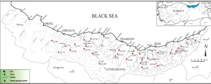
With respect to its river streamow, Turkey is divided into 26 basins [43]. Among them, the Black Sea Coast receives rainfall all the year round and also the greatest amount of rainfall in Turkey [44]. The EBSB is located on the northeastern coast of Turkey (Figure 1). The basin is surrounded by the Eastern Black Sea Mountains on the south and the Black Sea on the north. It averages nearly 1,100 mm annually; this gure can reach 2,300 mm near Rize Province. This region was selected as the study area since it has a great potential risk against oods due to its meteorological and topographic characteristics. Devastating ood events have occurred in the EBSB, especially in recent years. In this region, nearly 50 destructive oods have taken place between the years 1955 and 2010, causing 258 deaths and nearly US $500,000,000 of damage [44]. Therefore, reliable estimation of peak discharges is essential for the design of hydraulic structures and also for ood risk management.

Two types of data were used in this study: (i) streamow data (the annual maximum ood data) for RFFA and estimation of ood quantiles and (ii) physiographical, meteorological, and hydrological data for regression analysis techniques. The annual maximum ood data of 33 Stream-Gauging Stations (SGS) used in the study were obtained from both General Directorate of State Hydraulic works (DSI) and General Directorate of Electrical Power Resources and Development Administration (EIE). The locations of the stations used are shown in Figure 1. The longer the period of the record is, the more accurate

(4)

and representative statistical results will be in RFFA. Therefore, a minimum of ten years of SGSs were selected for the quality of the estimates. Record lengths of the selected 33 SGSs range 10-42 years (mean: 28 years). Flood quantiles of these stations were estimated for the selected return periods T = 5; 10; 25; 50; 100, and 500 years (Q5; Q10; Q25; Q50; Q100, and Q500) by

tting the best distribution with the region.

The selection of independent variables is a critical point in the estimation of ood discharges since they are inuenced by both physical and meteorological factors. Previous RA in RFFA studies was examined for the selection of independent variables. It was determined that most of them adapted drainage area (A), main stream slope (S), mean annual rainfall (R), stream density (D), and elevation (E) to RA, as presented in Table 1. Therefore, these variables were included in this study. Rainfall intensity (I) was also used in this study as an independent variable, since

it is known as an important meteorological parameter to aect the oods. However, there are few studies to include rainfall intensity in RA for RFFA [29,36].

The annual greatest precipitation values (mm) observed in various standard times, measured in ten meteorological stations in the region and obtained from Turkish State Meteorological Service (DMI), were used to calculate the rainfall intensities (I) [45]. Rainfall intensities were calculated by Aziz et al. [36] for various return periods with duration equal to time of concentration (in hours):

tc = 0:76A0:38;

where A is basin area (km2_{). The rainfall parameters}

for each SGS were calculated by Thiessen Polygons method. EASYFIT goodness of t procedure was adapted to rainfall intensities to determine the most appropriate distribution of the region. Then, using the

Table 1. Catchment characteristics of independent variables used in some previous studies.

Authors Country Method Independent variables adopted

Jingyi and Hall (2004) [20] China Index ood and ANN

A; R; S; E, main stream length, geological feature index, plantation cover index Shu and Burn (2004) [32] England, UK QR and ANN A; R, soil drainage type

Dawson et al. (2006) [33] Ireland RA and ANN A; R; S; E, base ow index, standard percentage run-o, longest drainage path

Leclerc et al. (2007) [24] Canada CCA A; R, gauging station latitude, gauging station longitude, mean air temperature

Shu and Ouarda

(2007, 2008) [34,35] Canada

CCA, ANN and ANFIS

A; R; S, fraction of the basin area covered with lakes, annual mean air temperature

Palmen and Weeks

(2011) [26] Australia QR

A; R; S; I; D, river length, sediment area, plantation area, evapotranspiration

Malekinezhad et al. (2011) [28] Iran Index ood and RA

R, Length of main waterway, compactness coecient, mean annual temperature Haddad et al. (2012) [29] Australia QR and RA A; R; I; D, mean annual evapotranspiration Aziz et al. (2013) [36] Australia QR and ANN A; R; S; I, evapotranspiration

Seckin et al. (2013) [14] Turkey RA and ANN A; E, latitude, longitude, return period

This study (2014) Turkey RA, ABC and

(5)

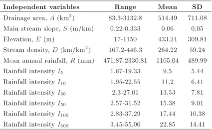
Table 2. Exploratory data analysis of the independent variables.

Independent variables Range Mean SD

Drainage area, A (km2₎ _83.3-3132.8 _514.49 _711.08

Main stream slope, S (m/km) 0.22-0.333 0.06 0.05 Elevation, E (m) 17-1150 433.24 309.81 Stream density, D (km/km2₎ _167.2-446.3 _264.22 _59.24

Mean annual rainfall, R (mm) 471.87-2330.81 1105.04 489.99 Rainfall intensity I5 1.67-19.33 9.5 5.44

Rainfall intensity I10 1.95-22.55 11.2 6.41

most appropriate distribution, rainfall intensity values were calculated for T = 5; 10; 25; 50; 100, and 500 years return periods (I5; I10; I25; I50; I100, and I500).

Drainage areas of SGS, ranging from 83.3 to 3,132 km2 _{(mean: 774.83 km}2_{), and elevations, ranging 17}

to 1,150 m (mean: 433.24 m), were obtained from DSI and EIE [46]. Mainstream slopes and stream density values were compiled from Saka [47].

In summary, the independent variables used in this study are: drainage area, A (km2_{), main stream}

slope, S (m/km), elevation, E (m), stream density, D (km/km2_{), mean annual rainfall, R (mm), and rainfall,}

intensities, I (mm/h) for T = 5; 10; 25; 50; 100, and 500 years. Ranges and summary statistics of these data are presented in Table 2.

3. Methodology

3.1. Estimation of ood quantiles

In all stages of RFFA, the identication of homoge-neous regions has great signicance. It is expected that the more homogeneous a region is, the more accurate the estimation will be in RFFA based on L-moments method [48]. The eciency of the regionalization is relatively dependent on the historical ow record length and the similarity of the hydrological characteristics of regions [49]. After identifying a homogeneous region, an appropriate distribution needs to be selected for the regional frequency analysis. Assessment of the goodness of dierent candidate distributions for a particular application will largely be based on how well the distributions t the available data. When several distributions t the data suciently, the best choice among them will be the distribution that is most robust [50].

In this study, homogeneity of the region was determined by discordancy (Di) and heterogeneity

measures (Hi) based on L-moments. The probability

distributions, whose parameters were computed by the

L-moments method, were Generalized Logistic (GLO), GEV, PE3, and LN distributions in the analysis ZDIST

statistics used for the goodness of t for each of 33 stations.

The fundamental quantity of statistical frequency analysis is the frequency distribution, which species how frequently the possible values of Q occur. The probability that the actual value of Q is at most x is denoted by F (x):

F (x) = Pr

Q x

: (1)

F (x) is the cumulative distribution function of the frequency distribution. Its inverse function, x(F ), the quantile function of the frequency distribution, expresses the magnitude of an event in terms of its nonexceedance probability F . The quantile of return period T , QT, is an event magnitude so extreme that

it has probability 1=T of being exceeded by any single event. For an extreme high event, in the upper tail of the frequency distribution, QT is given by:

F (Q(T )) =

1 1 T

; (2)

for an extreme low event, in the lower tail of the frequency distribution, the corresponding relations are QT = x(1=T ) and F (QT) = 1=T . The goal of

the frequency analysis is to obtain a useful estimate of quantile QT for a return period of scientic

rele-vance [51]. QT functions of the best-t distribution

were used for the estimation of quantiles related to T values of 5; 10; 25; 50; 100, and 500 years.

3.2. Selection of independent variables

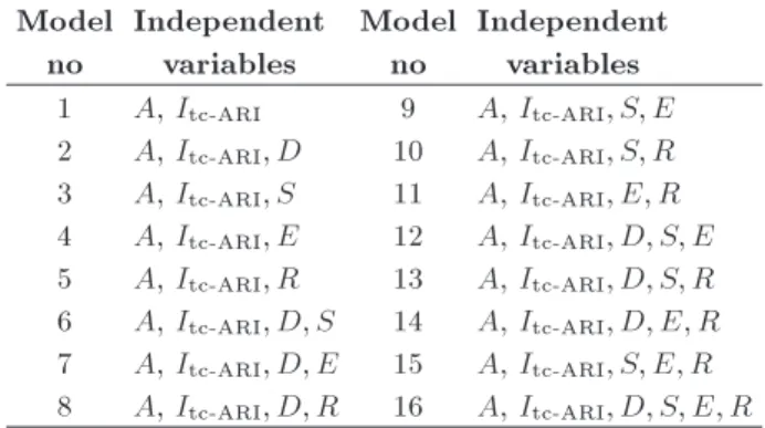
Regression analysis was applied to the data to get a set of variables that provides the best statistical model. 16 models expected to be signicant were developed for six variables. Drainage area and rainfall intensity were

(6)

Table 3. Models and independent variables used in the study.

Model no

Independent variables

Model no

Independent variables 1 A, Itc-ARI 9 A, Itc-ARI; S; E

2 A, Itc-ARI; D 10 A, Itc-ARI; S; R

3 A, Itc-ARI; S 11 A, Itc-ARI; E; R

4 A, Itc-ARI; E 12 A, Itc-ARI; D; S; E

5 A, Itc-ARI; R 13 A, Itc-ARI; D; S; R

6 A, Itc-ARI; D; S 14 A, Itc-ARI; D; E; R

7 A, Itc-ARI; D; E 15 A, Itc-ARI; S; E; R

8 A, Itc-ARI; D; R 16 A, Itc-ARI; D; S; E; R

found to be the most important predictor variables in the previous RFFA studies [36]. These models, which contain drainage area, rainfall intensity, and combinations of the other four-predictor variables, are shown in Table 3. The pre-calculated discharges for T = 5; 10; 25; 50; 100, and 500 years return periods were then adapted to the independent variables using a regression model. Regression analysis was applied to the data for the determination of discharges as a function of the catchment characteristics having the highest determination coecient (R2_{). In this analysis,}

each return period of discharges corresponds to the rainfall intensities with the same return periods.

Model 16 represents the best R2 _{values, and}

indicates that drainage area, stream frequency, stream slope, elevation, average annual rainfall, and rainfall intensity are signicant variables that greatly inuence the discharges. Further details of the model results were discussed by Anilan [52].

3.3. Articial Bee Colony (ABC) algorithm The ABC algorithm is a new population-based meta-heuristic approach proposed by Karaboga in [53]. The algorithm simulates the intelligent foraging behavior of honey bee swarms. In the ABC algorithm, the position of a food source represents a possible solution to the optimization problem and the nectar amount of a food source corresponds to the quality (tness) of the associated solution. In this study, the unknown coecients of regression functions are the parameters of a solution, and ABC algorithm tries to nd optimum coecients.

The ABC algorithm includes three control pa-rameters: the number of food sources (SN), equal to the number of employed or onlooker bees; the \limit"; and the Maximum Cycle Number (MCN) [54]. The algorithm generates a randomly distributed initial population of SN solutions (for food source position) by Eq. (3) and also evaluates the amount of nectar (tness) by Eq. (4):

xij = xminj + rand (0; 1)(xmaxj xminj ); (3)

ti=

(

1=(1 + fi) if fi 0

1 + abs(fi) if fi< 0 ; (4)

where i = 1 : : : SN; j = 1 : : : D; SN denotes the number of food sources or employed bees; D is the number of optimization parameters; xmin

j and xmaxj

are the lower and upper bounds of the jth parameter, respectively; fi is the value of the objective function.

Each employed bee searches for new food sources with more nectar in the neighborhood of its current food source by Eq. (5). Then, it evaluates its nectar amount (tness) by Eq. (4) [55]:

vij = xij+ ij(xij xkj); (5)

where k 2 f1; 2; : : : ; SNg and j 2 f1; 2; : : : ; Dg are randomly chosen indices, and k 6= i:'ij is a random

real number within [{1,1].

An onlooker bee chooses a food source depending on the probability values (Eq.(6)) calculated using the tness value provided by the employed bees:

pi=P_SNti

i=1ti; (6)

when a food source cannot be improved in a predeter-mined number of trials (the \limit"), then food source is abandoned by the employed bee, which becomes a scout and seeks a new source without using experi-ence [53]. A new food source position is generated randomly by Eq. (3), and the abandoned ones are replaced by scouts. The best food source is determined, and its position is memorized. This cycle is repeated until the requirements are met [56,57].

3.4. Teaching-Learning Based Optimization (TLBO) algorithm

Rao et al. rst developed a new meta-heuristic opti-mization algorithm based on the natural phenomenon of teaching and learning [58]. The TLBO algorithm has two common control parameters: the number of students (population size) and the stopping criterion (maximum number of iterations) [59]. Like other optimization algorithms, it uses a randomly generated initial population that consists of an even number of students, which are any solutions according to the population size and number of design variables in TLBO. These students consist of a number of design variables (Xi) that generate an initial population as

follows [60]: for i = 1 : Pn

for j = 1 : ng

randomly select any X between Xmin and Xmax student (i; j) = X

end for end for,

(7)

groups if the design variables are categorized, Xmin

and Xmax are the minimum and maximum values,

respectively, of the design variables of the regression functions in this study.

In the TLBO algorithm, a new population is obtained as a result of two basic stages: the \teacher phase" or learning from the teacher, and the \learning phase," or trade of information between learners [61]. In the teacher phase, the student, with minimum objective function, f, in the entire population, is found and mimicked as a teacher. Other students in the current population are modied as the neighborhood of the teacher using the following equations:

studenti=

Xi;1Xi;2:::Xi; Dn

i=1; 2; ::::; P n; (7)

mean=

mean (X1) mean (X2):::: mean (XDN)

; (8)

studentnew t=studenti+r(teacher T Fmean); (9)

where DN is the number of design variables, Pn is the

population size, r is a random number varying in [0,1], and T F is the teaching factor (1 or 2). Xi is the

unknown coecient of a regression function:

T F = round (1 + rand (2 1)): (10) The size of r must be equal to that of the student for the scalar multiplication given in Eq. (7). The teaching phase is carried out with the hope of upgrading the students' level to teachers' [60]. In the learning phase, modied students increase their knowledge by interacting with each other according to the teaching-learning process [59].

At the end of the learning phase, a cycle (iter-ation) is completed for the TLBO algorithm. The learning and teaching phases are continued until the termination criterion is reached [59]. Uzlu et al. [42] presented detailed information about the TLBO algo-rithm and its implementation.

4. Regional ood frequency analysis based on the ABC and TLBO algorithms

In the prediction process, three regression functions, i.e. Linear Function (LF, Eq. (11)), Power Func-tion (PF, Eq. (12)), and Exponential FuncFunc-tion (EF, Eq. (13)), were used to estimate the regional ood frequency for the EBSB, Turkey. The general form of LF, PF, and EF can be expressed as follows:

ylinear=w0+ w1x1+ w2x2+ w3x3

+ w4x4+ + wnxn; ₍₁₁₎

ypower= w0xw11xw22x3w3xw44: : : xbnn; (12)

yexponential=w0+ exp(w1+ w2x1+ w3x2+ w4x3

+ w5x4+ + wn+1xn); (13)

where y is the dependent variable, wis are the

regres-sion coecients, and xis are independent variables for

general signication. In this study, y corresponds to Q, and xis are drainage area (A), rainfall intensities (I),

stream density (D), mean annual rainfall (R), main stream slope (S), elevation (E), respectively.

Since the values of the independent variables are in extremely dierent ranges, optimization of the coecients will become so dicult. This is because some values will be too big and some too small. Therefore, each group of input and output values is normalized into the range between [0.1, 0.9] in the ABC and TLBO models as follows:

Normalized value =

Raw value - Min value Max value - Min value

(0:9 0:1) + 0:1: (14) The aim of estimating regional ood frequency is to nd the ttest model to the observed data. The equations for six parameters were evaluated using 33 experimen-tal data and the best equations with minimum SSE were determined. In addition, performances of ABC and TLBO models were compared using Mean Relative Error (MRE), Root Mean Square Error (RMSE), and Mean Absolute Error (MAE). MRE, RMSE, and MAE are calculated as follows:

MRE= 1 N

N

X

i=1

Ln(Q)iobserved Ln(Q)ipredicted

Ln(Q)iobserved

100;

(15)

RMSE=

1 N

N

X

i=1

1=2

; (16)

MAE = 1 N

N

X

i=1

; (17) where N is the number of elements in the series.

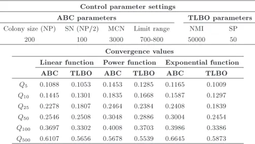
The parameters of the ABC algorithms were set to the same values for all models: colony size (NP) = 200, number of food sources (SN) = 100, limit = 700-800, and the maximum number of cycles was MCN = 3,000. On the other hand, control parameters of TLBO were adjusted as follows: number of maximum itera-tion (NMI)= 50,000 and size of populaitera-tion (SP)=50. Both TLBO and ABC parameters' ranges were set between [{5,5]. After setting control parameters, thirty independent runs were performed using TLBO and

(8)

Table 4. Control parameter settings and convergence values. Control parameter settings

ABC parameters TLBO parameters

Colony size (NP) SN (NP/2) MCN Limit range NMI SP

200 100 3000 700-800 50000 50

Convergence values

Linear function Power function Exponential function

ABC TLBO ABC TLBO ABC TLBO

Q5 0.1088 0.1053 0.1453 0.1285 0.1165 0.1009

Q10 0.1445 0.1301 0.1835 0.1668 0.1587 0.1297

Q25 0.2278 0.1807 0.2464 0.2384 0.2408 0.1839

Q50 0.2546 0.2508 0.3048 0.2886 0.3004 0.2454

Q100 0.3697 0.3302 0.4008 0.3703 0.3986 0.3386

Q500 0.6107 0.5656 0.5678 0.5539 0.6645 0.5873

ABC algorithms for each of dimensional and non-dimensional regression equations. Table 4 provides control parameters and convergence values used in ABC and TLBO algorithms.

5. Results and discussion

Homogeneity of the region was determined by discor-dancy measure (Di) and heterogeneity measure (Hi)

tests based on L-moments. As a result of these tests, ve of the stations which failed to pass the homogeneity criteria were extracted from consideration. The rest of 33 stations indicated that the region was homogeneous. There was no site identifying that Di value exceeded

the critical value of Dcr= 3 in these 33 stations. The

region was also considered homogeneous according to heterogeneity measure, as H1 (1.69) value took part

between Hcr ranging 1 to 2.

GLO, LN, PE3, and GEV distributions were

tted with the ood data of the homogeneous region. The parameters of these distributions were estimated by L-moments approach. ZDIST _{statistics goodness}

of t test expressed that the data of 33 stations t with LN distribution for the region. Seckin et al. (2011) accepted the GEV distribution for whole Turkey according to the ZDIST _{goodness of t test. In this}

study, LN distribution was approved for the EBSB. The reason for the dierence may be the fact that they applied the distribution to the heterogeneous region. Based on the appropriate distributions for each site, ood discharges were estimated for return periods of T = 5; 10; 25; 50; 100, and 500 years and represented as dependent variables for the regression analysis. QT

functions of the best-t distribution were used for the estimation of quantiles related to T values of 5, 10, 25, 50, 100, and 500 years. Summary of the L-moments statistics and ood quantiles is presented in Tables 5 and 6.

Table 5. Summary of L-moments statistics. Homogeneity measure

Divalues of 33 stations are between 0.14-2.85< Dcr= 3 (Di criteria by Hosking 1994)

Heterogeneity measure H1= 1:69

The region is possibly homogeneous 1 < Hi< 2(Hicriteria by Hosking 1994)

H2= 0:41

H3= 0:96

Values of ZDIST _{statistic of various distributions}

Distributions L-kurtosis ZDIST

Absolute Z-statistics value suciently closer to zero is the 0.33

with Ln distribution (Z-statistics criteria by

Hosking 1994) Log Normal (LN) 0.239 {0.33

Gen. Extreme Value (GEV) 0.212 {1.72 Gen. logistik (GLO) 0.191 {2.78 Pearson tip III (PE3) 0.156 {4.59

(9)

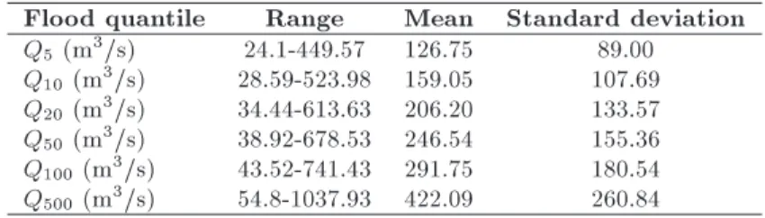
Table 6. Summary statistics of ood quantiles as dependent variables. Flood quantile Range Mean Standard deviation Q5 (m3/s) 24.1-449.57 126.75 89.00

Q10(m3/s) 28.59-523.98 159.05 107.69

Q20(m3/s) 34.44-613.63 206.20 133.57

Q50(m3/s) 38.92-678.53 246.54 155.36

Q100 (m3/s) 43.52-741.43 291.75 180.54

Q500 (m3/s) 54.8-1037.93 422.09 260.84

For developing the regional ood-prediction equa-tions, the relation of the ood quantiles of selected intervals and basin characteristics was determined by non-linear RA. 16 models expected to be signicant were developed for six variables. LP, PF, and EF were used in the non-linear RA. The results of dierent combinations showed that drainage area and rainfall intensity were the variables with the most signicant inuence on the performance of the model. R2 _values

appeared to signicantly decrease as the quantiles in-creased in all of 16 models as expected. This approach showed that the development of non-regression model using dierent independent variables leads to ecient models of dierent ood quantiles for the range of 5 to 500 years. On the basis of this assumption, MRE, RMSE, and MAE values were applied to Model 16 to evaluate the performance of regression analysis. In order to compare them with RA, the ABC and TLBO models were also developed for Model 16.

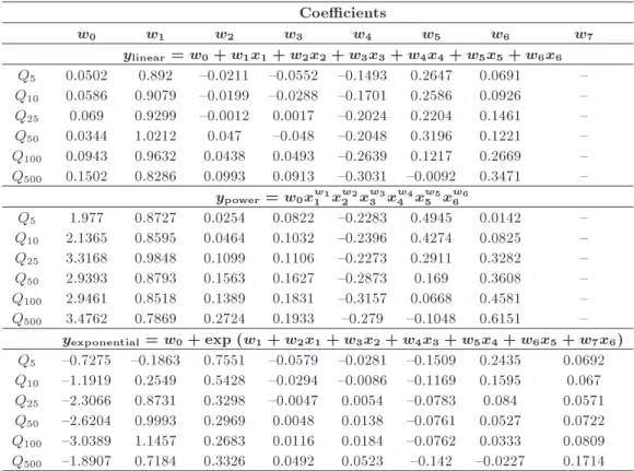
Similarly, six independent variables were related to ood quantiles and three functions were adapted to the model. The coecients obtained from the ABC and TLBO are presented in Tables 7 and 8,

respectively. Results of the analysis with RA, ABC, and TLBO were compared in terms of the MRE, MAE, and RMSE, as given in Table 9. Among all of the error values of dierent return periods, the smallest one was obtained through the exponential function for Q5with

the TLBO model as 23.42 (MAE) as marked in bold in Table 9.

As shown in the table, the analysis showed a reasonable performance, and the comparison with each other showed that results of the TLBO and ABC were superior to those of RA. Furthermore, when compared the ABC with TLBO, TLBO model outperformed ABC model in terms of RMSE values for all functions, while ABC presented better results in terms of RE values, except for exponential function. There were no signicant dierence observed between TLBO and ABC in terms of MAE values for the three functions. TLBO-EF was performed as the best model with the MRE = 26.87, MAE = 23.42, and RMSE = 29.41.

When they were generally considered for each return period (T = 5; 10; 25; 50; 100, and 500), MRE, RMSE, and MAE error values indicated that TLBO method gave better results for the estimation of ood

Table 7. Coecients obtained from ABC. Coecients

w0 w1 w2 w3 w4 w5 w6 w7

ylinear= w0+ w1x1+ w2x2+ w3x3+ w4x4+ w5x5+ w6x6

Q5 0.0013 0.9281 0.0138 {0.0728 {0.1191 0.3003 0.0728 {

Q10 {0.039 0.9652 0.0536 {0.0342 {0.106 0.3987 0.0384 {

Q25 0.057 1.008 {0.0413 {0.1462 {0.1854 0.4126 0.0072 {

Q50 {0.0203 1.016 0.0912 0.0096 {0.1721 0.3185 0.1533 {

Q100 {0.076 1.0788 0.16 0.0343 {0.1521 0.3489 0.1963 {

Q500 {0.0538 0.9677 0.2788 0.0773 {0.2028 0.1145 0.381 {

ypower= w0xw11xw22x3w3xw44xw55xw66

Q5 3.0383 1.0011 0.0077 0.0928 {0.1745 0.728 {0.033 {

Q10 2.9856 1.0187 0.0359 0.0882 {0.2043 0.4263 0.2173 {

Q25 3.9857 1.0245 0.1402 0.1707 {0.2576 0.2357 0.4237 {

Q50 3.2846 0.989 0.105 0.1622 {0.3203 0.0508 0.5546 {

Q100 2.2542 0.8708 0.0046 0.2208 {0.4241 {0.096 0.5833 {

Q500 2.8765 0.7379 0.2109 0.2558 {0.3612 {0.1302 0.6105 {

yexponential= w0+ exp (w1+ w2x1+ w3x2+ w4x3+ w5x4+ w6x5+ w7x6)

Q5 {0.3094 {1.0171 1.2824 0.0011 {0.0232 {0.16 0.3408 0.3076

Q10 {0.5406 {0.5813 1.0105 0.0438 {0.0208 {0.0989 0.1751 0.3021

Q25 {1.0501 {0.0072 0.7229 0.0751 0.0091 {0.0644 0.1124 0.2512

Q50 {0.5823 {0.5284 0.9689 0.1548 0.0342 {0.1434 0.067 0.443

Q100 {0.0937 {1.1584 1.3921 {0.0859 0.2376 {0.6509 0.044 0.6473

(10)

Table 8. Coecients obtained from TLBO. Coecients

w0 w1 w2 w3 w4 w5 w6 w7

ylinear= w0+ w1x1+ w2x2+ w3x3+ w4x4+ w5x5+ w6x6

Q5 0.0502 0.892 {0.0211 {0.0552 {0.1493 0.2647 0.0691 {

Q10 0.0586 0.9079 {0.0199 {0.0288 {0.1701 0.2586 0.0926 {

Q25 0.069 0.9299 {0.0012 0.0017 {0.2024 0.2204 0.1461 {

Q50 0.0344 1.0212 0.047 {0.048 {0.2048 0.3196 0.1221 {

Q100 0.0943 0.9632 0.0438 0.0493 {0.2639 0.1217 0.2669 {

Q500 0.1502 0.8286 0.0993 0.0913 {0.3031 {0.0092 0.3471 {

ypower= w0xw11xw22x3w3xw44xw55xw66

Q5 1.977 0.8727 0.0254 0.0822 {0.2283 0.4945 0.0142 {

Q10 2.1365 0.8595 0.0464 0.1032 {0.2396 0.4274 0.0825 {

Q25 3.3168 0.9848 0.1099 0.1106 {0.2273 0.2911 0.3282 {

Q50 2.9393 0.8793 0.1563 0.1627 {0.2873 0.169 0.3608 {

Q100 2.9461 0.8518 0.1389 0.1831 {0.3157 0.0668 0.4581 {

Q500 3.4762 0.7869 0.2724 0.1933 {0.279 {0.1048 0.6151 {

yexponential= w0+ exp (w1+ w2x1+ w3x2+ w4x3+ w5x4+ w6x5+ w7x6)

Q5 {0.7275 {0.1863 0.7551 {0.0579 {0.0281 {0.1509 0.2435 0.0692

Q10 {1.1919 0.2549 0.5428 {0.0294 {0.0086 {0.1169 0.1595 0.067

Q25 {2.3066 0.8731 0.3298 {0.0047 0.0054 {0.0783 0.084 0.0571

Q50 {2.6204 0.9993 0.2969 0.0048 0.0138 {0.0761 0.0527 0.0722

Q100 {3.0389 1.1457 0.2683 0.0116 0.0184 {0.0762 0.0333 0.0809

Q500 {1.8907 0.7184 0.3326 0.0492 0.0523 {0.142 {0.0227 0.1714

Table 9. MRE, MAE, and RMSE values. Regression Analysis (RA)

MRE MAE RMSE MRE MAE RMSE MRE MAE RMSE

Q5 25.54 24.54 30.0 30.48 29.74 38.5 33.34 26.14 31.9

Q10 26.90 31.38 38.9 33.14 39.75 50.9 35.26 35.40 42.9

Q25 29.64 43.08 53.6 36.31 54.94 69.5 37.90 49.82 60.6

Q50 32.75 55.87 68.1 38.73 68.28 85.9 39.81 62.05 77.3

Q100 36.18 70.82 87.3 41.56 83.90 105.1 42.62 77.25 98.4

Q500 47.88 126.14 160.9 46.05 145.56 178.5 53.34 130.01 175.7

Articial Bee Colony Algorithms (ABC)

Q5 23.92 24.25 30.53 23.72 26.98 35.29 27.36 24.96 31.6

Q10 25.17 31.57 40.98 23.7 34 46.18 27.47 33.03 42.94

Q25 24.67 46.49 60.15 27.88 47.81 62.55 30.57 48.39 61.84

Q50 29.72 54.54 70.22 30.27 57.71 76.84 33.09 58.34 76.28

Q100 33.77 72.2 92.34 33.61 73.07 96.14 37.99 74.02 95.88

Q500 45.41 126.84 167.17 44.71 126.86 161.2 44.94 123.9 174.38

Teaching-Learning Based Optimization (TLBO)

Q5 25.43 24.42 30.04 26.97 26.33 33.19 26.87 23.42 29.41

Q10 26.90 31.39 38.88 29.24 35.07 44.02 27.36 30.56 38.81

Q25 29.64 43.08 53.58 27.96 46.29 61.53 29.54 43.59 54.04

Q50 29.46 55.23 69.70 31.69 57.23 74.77 32.60 56.07 68.94

Q100 36.18 70.82 87.27 34.25 70.35 92.41 35.84 71.08 88.37

(11)

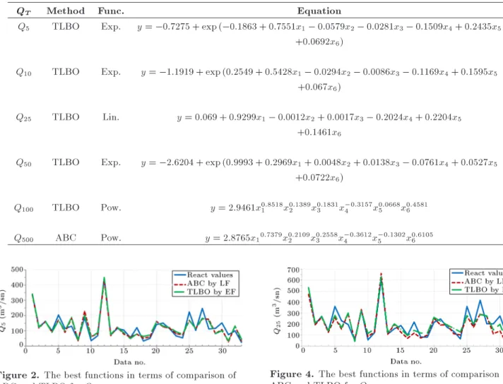
Table 10. Best equations for Q5; Q10; Q25; Q50; Q100; and Q500.

QT Method Func. Equation

Q5 TLBO Exp. y = 0:7275 + exp ( 0:1863 + 0:7551x1 0:0579x2 0:0281x3 0:1509x4+ 0:2435x5

+0:0692x6)

Q10 TLBO Exp. y = 1:1919 + exp (0:2549 + 0:5428x1 0:0294x2 0:0086x3 0:1169x4+ 0:1595x5

+0:067x6)

Q25 TLBO Lin. y = 0:069 + 0:9299x1 0:0012x2+ 0:0017x3 0:2024x4+ 0:2204x5

+0:1461x6

Q50 TLBO Exp. y = 2:6204 + exp (0:9993 + 0:2969x1+ 0:0048x2+ 0:0138x3 0:0761x4+ 0:0527x5

+0:0722x6)

Q100 TLBO Pow. y = 2:9461x0:85181 x0:13892 x0:18313 x40:3157x0:06685 x0:45816

Q500 ABC Pow. y = 2:8765x10:7379x0:21092 x0:25583 x40:3612x50:1302x0:61056

Figure 2. The best functions in terms of comparison of ABC and TLBO for Q5.

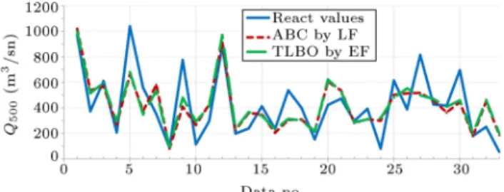
quantiles for dierent independent variables. The best-t equations for Q5; Q10; Q25; Q50; Q100, and Q500

obtained with the ABC and TLBO models are given in Table 10. Figures 2-7 also show the best functions in terms of comparison of ABC and TLBO.

6. Conclusion

The paper presents the application of the regression analysis, along with ABC and TLBO models to RFFA based on L-moments for the EBSB, Turkey. Based

(12)

on the L-moments approach, ood quantiles were estimated for return periods of T = 5; 10; 25; 50; 100, and 500 years. Moreover, these quantiles were used as dependent variables in the analysis. It has been found that Model 16, including the independent variables of drainage area, mainstream slope, mean annual rainfall, stream density, elevation, and rainfall intensity, out-performs other models with dierent combinations in terms of higher R2_{values. It has also been found that}

the choice of inputting independent variables to the model has a signicant impact on the estimation of dis-charges. For developing the regional ood-prediction equations, the relation of the ood quantiles of selected intervals and basin characteristics was determined by non-linear RA. In order to evaluate the performance of the RA in comparison with those of the ABC and TLBO methods, MRE, RMSE, and MAE measures were applied to the model. The results indicated that the TLBO and ABC outperformed the RA. TLBO-EF was performed as the best model with the MRE = 26.87, MAE = 23.42, and RMSE = 29.41. The results also further suggest that TLBO is superior to the ABC. The proposed equations obtained using the ABC and TLBO algorithms successfully estimate the ood quantile parameters. As the results of the TLBO algorithm were found to be satisfactory in this study, the use of the ABC and TLBO algorithm in hydrology is encouraged and recommended for future studies.

Acknowledgements

This paper is dedicated to the memory of the late Associate Professor Dr. Murat _Ihsan Komurcu, who passed away in February 2013.

References

1. Anilan, T., Satlms, U., Kankal, M., and Yuksek, O. \Application of articial neural networks and regres-sion analysis to L-moments based regional frequency analysis in the Eastern Black Sea Basin, Turkey", KSCE J. Civ. Eng., 20(5), pp. 2082-2092 (2016). 2. Jiapeng, H., Liang, Z., and Yu, Z. \A modied rational

formula for ood design in small basins", Journal of American Water Resources Association, 39(5), pp. 1017-1025 (2003).

3. Wallis, J.R. Risk and Uncertainties in the Evaluation of Flood Events for the Design of Hydraulic Structures, In Piene e Siccit, edited by E. Guggino, G. Rossi, E. Todini, pp. 3-36. Fondazione Politecnica del Mediter-raneo, Catania, Italy (1982).

4. Landwehr, J.M., Matalas, N.C., and Wallis, J.R. \Probability-weighted moments compared with some traditional techniques in estimating gumbel parame-ters and quantiles", Water Resour. Res., 15, pp. 1055-1064 (1979).

5. Hosking, J.R.M. \L-Moments: Analysis and estima-tion of distribuestima-tions using linear combinaestima-tions of order statistics", Journal of the Royal Statistical Society Series, B 52, pp. 105-124 (1990).

6. Rao, A.R. and Hamed, K.H. \Regional frequency analysis of Wabash River ood data by L-moments", J. Hydrol. Eng., 2(4), pp. 169-179 (1997).

7. Parida, B.P., Kachroo, R.K., and Shrestha, D.B. \Regional ood frequency analysis of Mahi-Sabarmati Basin using index ood procedure with L-moments", Water Resour. Manag., 12, pp. 1-12 (1998).

8. Adamowski, K. \Regional analysis of annual maximum and partial duration ood data by nonparametric and L-moment methods", J. Hydrol., 229, pp. 219-231 (2000).

9. Haktanir, T. \Comparison of various ood frequency distributions using annual ood peaks data of rivers in Anatolia", J. Hydrol., 136 (1-4), pp. 1-31 (1992). 10. Sorman, U. and Okur, A. \Application of at site and

regional frequency analyses by using the L-moments technique", _IMO Digest., 11(3), pp. 665-668 (2000). 11. Atiem, A. and Harmancoglu, N.B. \Assessment of

regional oods using L-moments approach: the case of the River Nile", Water Resour Manag., 20(5), pp. 723-747 (2006).

12. Saf, B. \Regional ood frequency analysis using L-moments for the Buyuk and Kucuk Menderes River Basins of Turkey", J. Hydrol. Eng., 14(8), pp. 783-794 (2009).

13. Bayazt, M. and Onoz, B. \LL-moments for estimating low ow quantiles", Hydrolog. Sci. J., 47(5), pp. 707-702 (2009).

14. Seckin, N., Cobaner, M., Yurtal, R., and Haktanir, T. \Comparison of ANN methods with L-moments for estimating ood ow at ungauged sites: The Case of East Mediterranean River Basin, Turkey", Water Resour. Manag., 27, pp. 2103-2124 (2013).

15. Aydogan, D., Kankal, M., and Onsoy, H. \Regional ood frequency analysis for Coruh Basin of Turkey with L-moments approach", J. Flood Risk Manage., 9, pp. 69-86 (2016).

16. Firat, M., Koc, A.C., Dikbas, F., and Gungor, M. \Identication of homogeneous regions and regional frequency analysis for Turkey", Sci. Iran., Transaction A, Civil Engineering, 21(5), pp. 1492-1502 (2014).

(13)

17. Fill, H.D. and Stedinger, J.R. \Using regional regres-sion within index ood procedures and an empirical Bayesian estimator", J. Hydrol., 210, pp. 128-145, (1998).

18. Pandey, G.R. and Nguyen, V.T.V. \A comparative study of regression based methods in regional ood fre-quency analysis", J. Hydrol., 225, pp. 92-101 (1999). 19. Ouarda, T.B.M.J., Girard, C., Cavadias, G.S., and

Bobee, B. \Regional ood frequency estimation with canonical correlation analysis", J. Hydrol., 254, pp. 157-173 (2001).

20. Jingy, I.Z. and Hall, M.J. \Regional ood frequency analysis for the Gan-Ming River Basin in China", J. Hydrol., 296, pp. 98-117 (2004).

21. Reis, J.R., D.S., Stedinger, J.R., and Martins, E.S. \Bayesian GLS regression with application to LPE3 regional skew estimation", Water Resour Res., 41, W10419 (2005). DOI: 10.1029/ 2004WR00344 22. Rahman, A. \A quantile regression technique to

estimate design oods for ungauged catchments in south-east Australia", Australian Journal of Water Resources, 9(1), pp. 81-89 (2005).

23. Gris, V.W. and Stedinger, J.R. \The use of GLS regression in regional hydrologic analysis", J. Hydrol., 344, pp. 82-95 (2007).

24. Leclerc, M. and Ouarda, T.B.M.J. \Non stationary re-gional frequency analysis at ungaged sites", J. Hydrol., 343, pp. 254-265 (2007).

25. Haddad, Kh., Rahman, A., Weinmann, P.E., Kucz-era, G., and Ball, J. \Streamow data preparation for regional ood frequency analysis: Lessons from southeast Australia", Australian Journal of Water Resources, 14(1), pp. 17-32 (2010).

26. Palmen, L.B. and Weeks, W.D. \Regional ood fre-quency for Queesland using the quantile regression technique", Australian Journal of Water Resources, 15(1), pp. 47-56 (2011).

27. Rahman, A., Haddad, K., Zaman, M., Kuczera, G., and Weinmann, P.E. \Design ood estimation in ungauged catchments: a comparison between the probabilistic rational method and quantile regression technique for NSW", Australian Journal of Water Resources, 14(2), pp. 127-137 (2011).

28. Malekinezhad, H., Nactnebel, H.D., and Klik, A. \Comparing the index ood and multiple regression methods using L-moments", Phys. Chem. Earth, 36, pp. 54-60 (2011).

29. Haddad, K. and Rahman, A. \Regional ood fre-quency analysis in Eastern Australia: Bayesian GLS regression-based methods within xed region and ROI framework-quantile regression and parameter regres-sion technique", J. Hydrol., 430-431, pp. 142-161 (2012).

30. Zaman, M.A., Rahman, A., and Haddad, K. \Regional ood frequency analysis in arid regions: A case study for Australia", J. Hydrol., 475, pp. 74-83 (2012).

31. Rezaeianzadeh, M., Tabari, H., Yazdi, A.A., Isik, S., and Kalin, L. \Flood ow forecasting using ANN, ANFIS and regression models", Neural Comput. Appl., 25(1), pp. 25-37 (2014).

32. Shu, C. and Burn, D.H. \Homogeneous pooling group delineation for ood frequency analysis using a fuzzy expert system with genetic enhancement", J. Hydrol., 291, pp. 132-149 (2004).

33. Dawson, C.W., Abrahart, R.J., Shamseldin, A.Y., and Wilby, R.L \Flood estimation at ungauged sites using articial neural networks", J. Hydrol., 319, pp. 391-409 (2006).

34. Shu, C. and Ouarda, T.B.M.J \Flood frequency anal-ysis at ungauged sites using ANN in canonical correla-tion analysis physiographic space" Water Resour Res., 43, W07438 (2007). DOI: 10.1029/2006WR005142 35. Shu, C. and Ouarda, T.B.M.J \Regional ood

fre-quency analysis at ungauged sites using the adaptive neuro-fuzzy inference system", J. Hydrol., 349, pp. 31-43 (2008).

36. Aziz, K., Rahman, A., Fang, G., and Shrestha, S. \Application of articial neural networks in regional ood frequency analysis: a case study for Australia", Stoch. Env. Res. Risk A., 28(3), pp. 541-554 (2014). 37. Chau, K.W. \Particle swarm optimization training

algorithm for ANNs in stage prediction of Shing Mun River", J. Hydrol., 329, pp. 363-367 (2006).

38. Jiong-feng, C., and Wan-chang, Z. \Application of genetic algorithm for model parameter calibration in daily rainfall-runo simulations with the Xinanjiang model", Journal of China Hydrology, 26(4), pp. 32-38 (2006).

39. Jun, Z., Chuntian, C., Jianjian, S., and Shiqin, Z. \Ant colony optimization-based support-vector machine for mid-and-long term hydrological forecasting", Journal of Hydroelectric Engineering, 06 (2010).

40. Kisi, O., Ozkan, C., and Akay, B. \Modeling discharge-sediment relationship using neural networks with arti-cial bee colony algorithm", J. Hydrol., 428-429, pp. 94-103 (2012).

41. Salimi, S., Mahmoodi, H., and Barahman, N. \Weekly-discharge estimation for Tang-Karzin's station, using MLP network optimized by ABC algorithm" Interna-tional Journal of Basic and Applied Science, 02(02), pp. 242-253 (2013).

42. Uzlu, E., Kankal, M., Akpinar, A., and Dede, T. \Estimates of energy consumption in Turkey using neural networks with the teaching-learning-based opti-mization algorithm." Energy, 75, pp. 295-303 (2014). 43. Yerdelen, C. \Change point of river stream ow in

Turkey." Sci. Iran., Transaction A, Civil Engineering, 21(2), p. 306 (2014).

44. Yuksek, O., Kankal, M., and Ucuncu, O. \Assessment of big oods in the Eastern Black Sea Basin of Turkey" Environmental Monit Assess, 185, pp. 797-814 (2013).

(14)

45. DMi, Analysis of Turkey's Maximum Precipitation Values and their Return Periods, Ankara, Turkey: Turkish State Meteorological Service (2001).

46. DSi \Annual ood reports" Ankara, Turkey, General Directorate of State Hydraulic Works (1970-2005). 47. Saka, F. \Determination of synthetic ow duration

curves by using mathematical methods and a case study in the Eastern Black Sea" PhD Thesis, Karad-eniz Technical University, Turkey (2012).

48. Yang, T., Shao, Q., Hao, Z.C., Chen, X., Zhang, Z., Xu, C.Y., and Sun, L. \Regional frequency analysis and spatio temporal pattern characterization of rainfall extremes in Pearl River Basin, China", J. Hydrol., 380, pp. 386-405 (2010).

49. Nyeko-Ogiramoi, P., Willems, P., Mutua, F.M., and Moges, S.A. \An elusive search for regional ood fre-quency estimates in the River Nile Basin", Hydrology and Earth System Sciences, 16, pp. 3149-3163 (2012). 50. Hosking, J.R.M. \On the characterization of distri-butions by their L-moments", Journal of Statistical Planning and Inference, 136, pp. 193-198 (2004). 51. Hosking, J.R.M. L-Moments, John Wiley & Sons, Inc.

(1998).

52. Anilan, T. \Application of articial intelligence meth-ods to L-moments based regional frequency analysis in the Eastern Black Sea Basin", PhD Thesis, Karadeniz Technical University, Turkey (2014).

53. Karaboga, D. \An idea based on honey bee swarm for numerical optimization", Technical Report- TR06, Erciyes University Engineering Faculty of Computer Engineering Department (2005).

54. Ozturk, H.T. and Durmus, A. \Optimum cost design of RC columns using articial bee colony algorithm", Struct. Eng. Mech., 45(5), pp. 643-54 (2013).

55. Pan, Q.K., Tasgetiren, M.F., Suganthan, P.N., and Chua, T.J. \A discrete articial bee colony algorithm for the lot-streaming ow shop scheduling problem", Inf. Sci., 181, pp. 2455-60 (2011).

56. Karaboga, D. and Basturk, B. \Articial bee colony (ABC) optimization algorithm for solving constrained optimization problems", Found Fuzzy Log Soft Com-put, 4529, pp. 789-798 (2007).

57. Uzlu, E., Akpnar, A., Ozturk, H.T., Nacar, S., and Kankal, M. \Estimates of hydroelectric generation us-ing neural networks with ABC algorithm for Turkey", Energy, 69, pp. 638-647 (2014).

58. Rao, R.V., Savsani, V.J., and Vakharia, D.P. \Teaching-learning based optimization: A novel

method for constrained mechanical design optimiza-tion problems", Computer-Aided Design, 43, pp. 303-315 (2011).

59. Togan, V. \Design of planar steel frames using teaching-learning based optimization", Eng. Struct., 34, pp. 225-32 (2012).

60. Togan, V. \Design of pin jointed structures using teaching learning based optimization", Struct. Eng. Mech., 47, pp. 209-225 (2013).

61. Dede, T. \Optimum design of grillage structures to LRFD-AISC with teaching-learning based optimiza-tion", Structural and Multidisciplinary Optimization, 48, pp. 955-964 (2013).

Biographies

Tugce Anlan is an Assistant Professor in Civil Engi-neering Department in Karadeniz Technical University, Trabzon, Turkey. Her current research focuses on ood frequency analysis, oods and sea outfalls.

Ergun Uzlu received BS, MS, and PhD degrees in Civil Engineering from Karadeniz Technical University, Trabzon, Turkey in 2008, 2011, and 2016, respectively. He is currently a Research Assistant in Karadeniz Technical University, Trabzon, Turkey. His research interests include coastal engineering, energy estimate models, and articial intelligence techniques.

Murat Kankal is an Assistant Professor in Civil Engineering Department in Karadeniz Technical Uni-versity, Trabzon, Turkey. His current research focuses on sediment transport in coastal area, regional ood frequency analysis, hydropower, and articial neural networks.

Omer Yuksek was born in Caykara, Trabzon, Turkey in 1962. He graduated from Maras Village Primary School, from Caykara _Inonu Secondary School, from Trabzon Religious Vocational High School, and from Karadeniz Technical University (KTU) Engineering Faculty (EF) at Civil Engineering Department (CED). He completed Post Graduate and Doctorate Educa-tions in KTU CED Hydraulic Division (HD) in 1986 and 1992, respectively. He studied in KTU EF CED HD as a Research Assistant between 1984-1993, as an Assistant Professor between 1993-1996, as an Associate Professor between 1996-2005, and as a Professor from 2005 until now. He is the Head of Hydraulic Division.