4826.pdf

(1)

Statistical Analysis of Symmetric Positive-definite Matrices

Ying Yuan

A dissertation submitted to the faculty of the University of North Carolina at Chapel Hill in partial fulfillment of the requirements for the degree of Doctor of Philosophy in the Department of Statistics and Operations Research (Statistics).

Chapel Hill 2011

Approved by:

Hongtu Zhu, Advisor

J. S. Marron, Advisor

Joseph. G. Ibrahim, Committee Member

Weili Lin, Committee Member

(2)

c

2011

Ying Yuan

(3)

Abstract

YING YUAN: Statistical Analysis of Symmetric Positive-definite Matrices. (Under the direction of Hongtu Zhu and J. S. Marron.)

This dissertation is motivated by addressing the statistical analysis of symmetric positive definite

(SPD) matrix valued data, which arise in many applications. Due to the nonlinear structure of

such data, it is challenging to apply well-established statistical methods to them. Our goal is to

develop statistical models and perform statistical inferences on the Riemannian manifold of the

space of SPD matrices. This dissertation has three major parts.

In the first part, we develop a local polynomial regression model for the analysis of data with

SPD matrix responses on the Riemannian manifold. The independent variable of this model is from Euclidean space. We examine two commonly used metrics including the affine invariant metric and

the Log-Euclidean metric on the space of SPD matrices. Under each metric, we develop an

asso-ciated cross-validation bandwidth selection method, and derive the asymptotic bias, variance, and

normality of the intrinsic local constant and local linear estimators and compare their asymptotic

mean square errors. Simulation studies are further used to compare the estimators under the two

metrics and examine their finite sample performance.

In the second part, we develop a functional data analysis framework to model diffusion tensors

along fiber bundles as functional responses with a set of covariates of interest, such as age,

diagnos-tic status and gender, in real applications. We propose a statisdiagnos-tical model with varying coefficient functions to characterize the dynamic association between functional SPD matrix-valued responses

and covariates. We calculate a weighted least squares estimation of the varying coefficient functions

under the Log-Euclidean metric in the space of SPD matrices. We also develop a global test

statis-tic to test specific hypotheses about these coefficient functions and construct their simultaneous

confidence bands. Simulated data are further used to examine the finite sample performance of the

(4)

The third part is to develop a varying coefficient model framework under the affine invariant

metric. This framework is very similar to that in the second part. However, this metric is more

complex than the Log-Euclidean metric, which makes the subsequent estimation of the varying coefficient functions and the theoretical derivations very challenging. Since there is no explicit form

formula for the estimators, we developed an optimization method for calculating it. We also derive

the asymptotic properties for the estimated coefficient functions, which are important for

construct-ing the simultaneous confidence band and the global test statistic. Moreover, comparisons of the

statistical powers of the varying coefficient models under the affine invariant and Log-Euclidean

metrics are made by using simulated data.

Keywords: Symmetric positive definite matrix, Log-Euclidean metric, affine invariant metric, Lo-cal polynomial regression, Functional data analysis, Varying coefficient model, Global test statistic,

(5)

Acknowledgments

This is a great opportunity to extend my deepest appreciation to all who were involved in the

completion of this dissertation.

First of all, I am sincerely grateful to my advisors, Professor Hongtu Zhu and Professor J. S.

Marron for their encouragement, direction and support. Throughout my dissertation work, they

continually stimulated my analytical thinking through discussions and greatly assisted me with

scientific writing. I improved myself a lot in formulating scientific problems and in developing

methods to solve these problems.

I would like to thank my committee members, Professor Joseph G. Ibrahim, Professor Weili Lin and Professor Haipeng Shen for their insightful suggestions on this dissertation that led me to

greatly improve my work.

Special thanks to Professor Martin Styner and Professor John H. Gilmore from Department of

Psychiatry at UNC-Chapel Hill for kindly providing the data that led to interesting applications

and Professor Pew-Thian Yap from Department of Radiology for helping with visulization.

Last, but not the least, I would like to express my gratitude to my family, who has been a

constant source of love, concern, support and strength all these years. To my parents for their

unconditional love and support. To my wonderful husband for listening to me, understanding me,

(6)

List of Figures

1.1 Ellipsoidal representations of DT’s along the splenium tract . . . 2

2.1 Ellipsoidal representations of the simulated SPD matrix data . . . 27

2.2 Ellipsoidal representations of the true and estimated SPD matrix data . . . 28

2.3 Boxplots of the AGD using the intrinsic local estimators . . . 29

2.4 log₁₀(LAGD) curves at each sample point using the intrinsic local estimators . . . . 30

2.5 Boxplots of the AGD using the intrinsic local linear estimators . . . 31

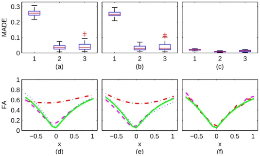
2.6 log₁₀(LAGD) curves at each sample point using the intrinsic local linear estimators . 32 2.7 Boxplot of the MADE’s using the three smoothing methods . . . 33

2.8 The splenium of the corpus callosum in the analysis of HIV DTI data . . . 34

2.9 Ellipsoidal representations of the diffusion tensor data and estimated tensors . . . . 34

2.10 FA’s, MD’s and PE’s . . . 35

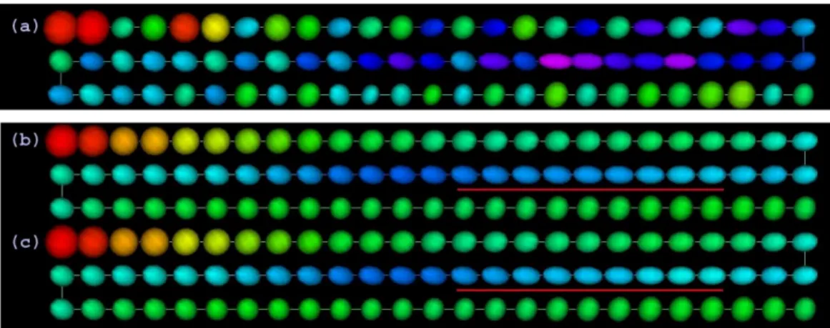
2.11 Ellipsoidal representations of estimated mean tensors . . . 36

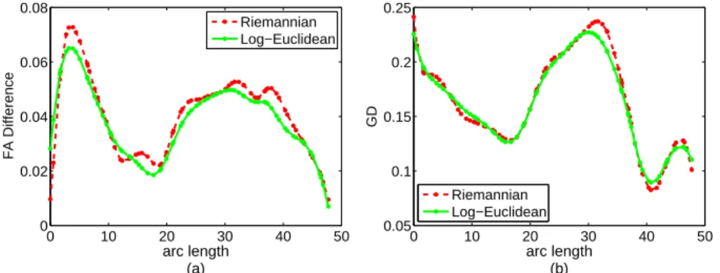
2.12 FA differences and geodesic distances . . . 36

3.1 The right internal capsule tract . . . 39

3.2 Ellipsoidal representations of the true, simulated and estimated diffusion tensors . . 52

3.3 Geodesic distances between simulated and estimated diffusion tensors . . . 52

3.4 Simulation study: Type I and Type II error rates . . . 54

3.5 Typical 95% simultaneous confidence bands for vectors of coefficient functions . . . . 56

3.6 Simulated coverage probabilities for D(z, β(x)) . . . 57

3.7 −log₁₀(p) values of test statisticsTn(xj) for testing gender or gestational age effect . 58 3.8 Ellipsoidal representations of raw and smoothed diffusion tensors . . . 59

3.9 95% simultaneous confidence bands for coefficient functions . . . 60

3.10 95% critical values forD(z, β(x)) over gestational ages for female and male groups . 61 4.1 Ellipsoidal representations of the simulated, true and estimated diffusion tensors . . 75

(10)

4.3 Simulation study: Type I and Type II error rates . . . 77

4.4 Typical 95% simultaneous confidence bands for vectors of coefficient functions . . . . 79

4.5 −log₁₀(p) values of test statisticsTn(xj) for testing gender or gestational age effect . 81

(11)

List of Tables

3.1 Simulated coverage probabilities for coefficient functions: VCLE methods . . . 55

4.1 Bias and standard deviation (SD) for coefficient functions . . . 76

(12)

Chapter 1 Introduction

Symmetric positive-definite (SPD) matrix-valued data occur in a wide variety of important

applications. For instance,

(1) An approach to computational anatomy has a representing shape in terms of deformation,

where a SPD deformation vector (J JT)1/2is computed to capture the directional information of shape change encoded in the Jacobian matricesJ at each location in an image (Grenander and Miller, 2007).

(2) An different type of computational anatomy is done in diffusion tensor imaging (DTI) (Basser

et al., 1994b), where a 3×3 SPD diffusion tensor (DT), which tracks the effective diffusion of

water molecules, is estimated at each voxel (a 3 dimensional (3D) pixel) of an imaging space.

(3) Brain function is studied in functional magnetic resonance imaging (fMRI), where a SPD

covariance matrix is calculated to delineate functional connectivity between different neural

assemblies when the subject is performing a complex cognitive task or perceptual process

(Fingelkurts et al., 2005; Gao et al., 2009).

(4) In classical multivariate statistics, a fundamental task is to model and estimate SPD

co-variance matrices for multivariate measurements, longitudinal data, time series data, among

many others (Pourahmadi, 1999, 2000; Anderson, 2003).

In this dissertation, we consider the situation where the data at hand are random SPD

matrix-valued samples instead of parameters like in the fourth application. Specifically, we focus on two

(13)

One example application is in DTI, where we obtained: (1) DT’s measured along a fiber tract as

a function of locations; (2) a collection of DT’s along a fiber tract measured as a function of age,

diagnostic status, and gender, while controlling for other clinical variables.

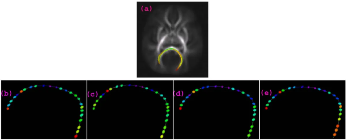
Figure 1.1 (a) displays one fiber tract in the brain, called the splenium tract projected onto a

slice of the FA image from a DTI scan. Along this tract, we have DT’s for each of different subjects

with some specific attributes, such as age, gender and diagnostic status. Each DT is geometrically

represented by an ellipsoid (Figure 1.1 (b)-(e)). In this representation, the lengths of the semiaxes

of the ellipsoid equal the square root of the eigenvalues of a DT, while the eigenvectors define the

direction of the three axes.

Figure 1.1: (a) shows the splenium tract extracted from the tensor atlas projected onto one axial slice of the FA image from a DTI scan, with color representing FA value. (b)-(e) shows the ellipsoidal representations of DT’s along the tract for four selected subjects, with some attributes such as age, gender and diagnostic status, etc..

Four issues arise when we deal with SPD matrix-valued data statistically.

(1) Should the analysis procedure be based on the derived scalar quantities or be based on the whole SPD matrices?

(2) Should the estimation be parametric or nonparametric?

(3) which metric should be used, Euclidean or non-Euclidean metrics?

(4) Which statistical model should be developed for a collection of SPD matrix-valued curves,

(14)

In current practice, many statistical analyses of SPD matrix valued data are based on the

derived scalar quantities or carried out for each individual element of SPD matrices (Smith et al.

(2006); O’Donnell et al. (2009); Gao et al. (2009)). For instance, in DTI, classical statistical methods are applied to fractional anisotropy values (FA is one derived quantity of a diffusion

tensor) along the fiber tracts in order to investigate the change of FA’s. And, in fMRI, they are

applied to regional correlation data in order to explore the development curve of each

inter-regional correlation. This is relatively simple and straightforward because many classical statistical

methods developed for data on Euclidean space can be directly applied in this situation. However,

this method of analysis is not adequate for investigating SPD matrix valued data or their derived

scalar quantities because they only use of part of the information from SPD matrices and so may

not reveal some important characteristics of the data. Moreover, the derived scalar quantities are

linear or nonlinear functions of the estimated eigenvalues of the SPD matrices and thus contain inherent bias. Hence, estimation and inference based on them can be substantially misleading. Our

simulation results will make this point clearly. Improvements will be made by developing statistical

methods that model the whole SPD matrix as a multivariate unit in this dissertation.

For Data type (i), we have SPD matrix-valued data measured at different spatial locations

(or different time points). We wish to denoise the data and reconstruct the underlying SPD

matrix-valued function. As is known (Fan and Gijbels (1996)), when some assumed underlying

functional forms and distributions are correct, a parametric method is better than a nonparametric

method in terms of computational speed and convergence rate of the estimator. However, the

reality is that the correct model is rarely available. In this situation, the performance of parametric methods can be very poor and inference based on incorrect assumptions about functional forms and

distributions can be highly doubtful. Nonparametric statistical methods can reduce the reliance

on the assumptions required for estimation and inference, thereby reducing the opportunities for

obtaining misleading results. One contribution of this dissertation is developing a nonparametric

regression method for the analysis of data with SPD matrix valued responses. Specifically, we

develop the local polynomial regression method for SPD matrix valued data, which can be used

to reconstruct the average change of SPD matrices as a function of some covariate, e.g. spatial

(15)

Here we mention three metrics. One is the Euclidean metric and the other two are non-Euclidean

metrics: the Log-Euclidean and affine invariant metrics (Arsigny (2006) and Schwartzman (2006)).

They correspond to three different geometries: the Euclidean, Log-Euclidean and affine invariant geometries. If we analyze SPD matrix valued data using the Euclidean metric, the usual estimation

methods widely studied on Euclidean spaces can be directly applied to them. However, this direct

application cannot guarantee the positive-definiteness of the estimates since the estimation highly

depends on the noise structure and the structure of the SPD matrices. It is possible to find

the closest points on the space of SPD matrices to the non-positive estimators. This falls into

the category of extrinsic methods. However, in general, extrinsic methods do not perform well,

especially for the statistical inference (Fletcher (2004)). In contrast, estimations using the

Log-Euclidean or affine invariant metrics do not suffer from this problem since the operations are carried

out by considering the space as a non-Euclidean space, which are intrinsic methods. Hence, in this work, we develop statistical methods with respect to the above two non-Euclidean metrics. Our

simulation results also show that in some scenarios, for example at moderate noise levels or for

non-gaussian noises, the estimators using the Euclidean metric fail to be SPD matrices and thus cannot

outperform those using the Log-Euclidean or affine invariant metrics. Moreover, even if using the

Euclidean metric can retain the positive-definiteness in some cases, estimators using this metric

suffer from the swelling effect, i.e. the determinant of the Euclidean estimators can be larger than

the original determinants. As said in Fletcher (2004), in DTI, diffusion tensors are assumed to be

covariance matrices of the local Brownian motion of water molecules. Introducing more dispersion

in computations amounts to introducing more diffusion, which is physically unacceptable.

For Data type (ii), we have a collection of SPD matrix-valued data measured along a curve (a

temporal or spatial curve) as a function of age, diagnostic status, and gender, while controlling

for other clinical variables. These data are in essence functional data. Moreover, one of the main

characteristics of these data is the combination of longitudinal or spatial information (time series or

spatial data) with cross-sectional information (attribute data). Data can contain trends that vary

in longitudinal or spatial aspects, that vary across different groups of subjects or objects. Take the

study of fiber tract in DTI as an example. There, each subject is characterized by a set of DT’s

(16)

data analysis (FDA). Compared with the classical statistics where the interest centers around a set

of data vectors, FDA can capture trend, processes and dynamic information which are inherent in

the data and thus increase the statistical power in detecting interesting features and in exploring variability. While there is extensive interest in developing FDA methods, however, most research

focuses are on functional data with the responses in Euclidean space. The functional data in this

dissertation have SPD matrix-valued responses, which lie in a non-Euclidean space. Those methods

for the data on Euclidean space cannot be directly applied.

Another major contribution of this dissertation is the development of varying coefficient model

frameworks for the analysis of SPD matrix valued functions and their association with a set of

covariates of interest, such as age, diagnostic status and gender, in real applications. Our modeling

will be formulated under the two affine invariant metrics mentioned above. The varying coefficient

model framework consists of four integrated components:

(i) a varying coefficient model for characterizing the association between SPD matrix valued

functions with a set of covariates of interest,

(ii) the local polynomial regression method for estimating the coeffient functions in the model,

(iii) global and local test statistics for testing hypotheses of interest

(iv) a resampling or χ2 approximation method for approximating the p-value of the global test statistic.

The remainder of this dissertation is organized as follows. In Chapter 2, we develop an intrinsic

local polynomial regression model for SPD matrix valued data under two Riemannian metrics:

affine invariant and Log-Euclidean metrics. Under each metric, we develop an associated

cross-validation method for nonparametric analysis of random SPD matrix-valued data and investigate

the asymptotic properties of the estimators. Simulation studies are performed to examine the finite sample performance of the estimator. In Chapter 3, we establish the varying coefficient

model framework under the Log-Euclidean metric, called VCLE, for analysis of the association

between fiber bundle diffusion tensors and a set of covariates of interest. Under this metric, a

varying coefficient model is formulated and correspondingly, an estimation procedure based on the

(17)

develop both local and global test statistics to test hypotheses on the varying coefficient functions

and a resampling method is used to approximate the p-value of the test statistics. We construct

a simultaneous confidence band to quantify the uncertainty in the estimated coefficient functions and propose a resampling method to approximate the critical point. We examine the finite sample

performance of VCLE via simulation studies. In Chapter 4, we formulate the varying coefficient

model framework developed in Chapter 3 under another commonly used metric for the space of

SPD matrices, the affine invariant metric, called VCAI. Specification of the model under this

metric involves the matrix exponential transformation and thus brings many more theoretical and

computational difficulties than that in Chapter 3. We develop an annealing evolutionary stochastic

approximation Monte Carlo algorithm for computing the coefficient functions (Liang (2010)). We

also derived the asymptotic properties of the coefficient functions, based on which a global test

(18)

Chapter 2 Local Polynomial Regression for SPD Matrices

2.1 Introduction

Symmetric positive-definite (SPD) matrix-valued data occur in many applications. This has motivated the recent development of several methods for statistical analysis of SPD matrices as

response variables in a Riemannian manifold. Schwartzman et al. (2008) has proposed several

parametric models for SPD matrices and derived the distributions of several test statistics for

comparing differences between the means of the two (or multiple) groups of SPD matrices. Kim

and Richards (2010) have developed a nonparametric estimator for the common density function

of a random sample of positive definite matrices. Zhu et al. (2009) develop a semi-parametric

regression model with SPD matrices as responses in a Riemannian manifold and covariates in a

Euclidean space. This model extends the two-group models studied by Schwartzman (2006) and

Schwartzman et al. (2008) to allow for general covariates and generalizes the parametric modeling in Schwartzman (2006) by assuming only that certain appropriately defined residuals have mean zero.

Barmpoutis et al. (2007) and Davis et al. (2010) have proposed tensor splines and local constant

regressions for interpolating DTI tensor fields based on the affine invariant metric, but these two

papers do not address several important issues of analyzing random SPD matrices including the

asymptotic properties of the nonparametric estimate proposed. Recently, Dryden et al. (2009)

compare the various choices of metrics of the space of SPD matrices and their properties.

To the best of our knowledge, this is the very first paper for developing an intrinsic local

polynomial regression (ILPR) model for estimating an intrinsic conditional expectation of a SPD

matrix response,S,given a covariate vectorxfrom a set of observations (x1, S1),· · · ,(xn, Sn), where

(19)

tract (e.g., right internal capsule tract), the coordinates in the 3D imaging space, and demographic

variables such as age. Important applications of ILPR include smoothing diffusion tensors along

fiber tracts and diffusion tensor fields, quantifying the change of diffusion and deformation tensors across groups and along time, and the evolution of inter-regional functional connectivity matrix

with time.

Compared with the existing literature, we make several contributions in this chapter. Since the

space of SPD matrices is a curved space, the standard local polynomial regression method is not

adequate and can lead to an unpleasant effect in image processing (Chefd’hotel et al., 2004). To

account for the curved nature of the SPD space, we consider the affine invariant metric and the

Log-Euclidean metric for the space of SPD matrices in order to examine the effect of different metrics on

carrying out statistical inference in the Riemannian manifold. Under each metric, we develop the

ILPR method for estimating the intrinsic conditional expectation of random SPD responses given the covariate and derive an approximation to its associated cross-validation method for bandwidth

selection. We establish the asymptotic properties of the ILPR estimators. We show the superiority

of the intrinsic local linear estimator over the intrinsic local constant estimator by examining their

asymptotic mean square errors. As shown in Figure 2.7 in Section 2.5, substantial improvements

can be made by treating SPD matrices in the Riemannian manifold.

The rest of this chapter is organized as follows. In Section 2.2, we develop the ILPR method

and its associated cross-validation method for nonparametric analysis of random SPD matrix-valued

data. We investigate the asymptotic properties of the estimators proposed under the affine invariant

metric in Section 2.3 and the Log-Euclidean metric in Section 2.4, respectively. We examine the finite sample performance of the estimator via simulation studies in Section 2.5. Finally, we will

analyze a real data set to illustrate a real-world application of the proposed ILPR method in Section

2.6 before offering some concluding remarks in Section 2.7.

2.2 Intrinsic Local Polynomial Regression for SPD matrices

Let Sym+(m) and Sym(m) be, respectively, the set of m×m SPD matrices and the set of

m×m symmetric matrices with real entries. Suppose that (xi, Si), i= 1,· · · , nis an independent

(20)

focus on a univariate covariate throughout the paper. The question of interest is to estimate an

‘intrinsic conditional expectation’ of S at each x, denoted by D(x), in Sym+(m).

Since Sym+(m) is a curved space, one cannot directly define D(x) =E(S|X =x) for a random SPD matrixS ∈Sym+(m). Instead, we introduce anm×mresidual matrix ofS atD(x), denoted by E_D(x), in Sym(m). The space Sym(m) is a Euclidean space with the Euclidean inner product given by < A1, A2 >= tr(A1A2) for any A1, A2 ∈ Sym(m). Thus, since ED(x) is in a Euclidean

space, we can directly compute its conditional expectation, which leads to the definition of ‘intrinsic

conditional expectation’ of S at each x as follows:

E{ED(X)|X =x}=Om, (2.2.1)

where Om is the m×m matrix with all elements zero. Heuristically, consider S and D(x) as

lying in Euclidean space, then ED(x) could be defined as S−D(x) and (2.2.1) would reduce to D(x) =E(S|X=x).

To rigorously define ED(X), we review some basic facts about the geometrical structure of

Sym+(m) in order to introduceaddition andsubtraction operations in Sym+(m) (Zhu et al., 2009; Schwartzman, 2006; Dryden et al., 2009). We first introduce the tangent vector and tangent space

at D(x) in Sym+(m). For a small scalar δ > 0, let C(t) be a differentiable map from (−δ, δ) to Sym+(m) passing through C(0) =D(x). A tangent vector at D(x) is defined as the derivative of the smooth curveC(t) with respect to tevaluated att= 0. The set of all tangent vectors atD(x) forms the tangent space of Sym+(m) at D(x), denoted asTD(x)Sym+(m). We need to introduce a specific metric<< ·,·>>D(x) as an inner product for tangent vectors on TD(x)Sym+(m). For the given metric, we can calculate<< UD(x), VD(x) >>D(x) for anyUD(x) andVD(x)on TD(x)Sym+(m) and then measure the length of the curve in Sym+(m). Furthermore, one can compute the shortest path, called the geodesic, between points in Sym+(m). Let γ_D₍_x₎(t, U_D₍_x₎) be the geodesic as a function of tpassing throughγ_D₍_x₎(0, U_D₍_x₎) =D(x) in the direction ofU_D₍_x₎∈T_D₍_x₎Sym+(m).

(21)

TD(x)Sym+(m). We define an open sphere of radiusrcentered at the ‘origin’D(x) inTD(x)Sym+(m) as

BD(x)(r) ={UD(x)∈TD(x)Sym+(m) :<< UD(x), UD(x)>>D(x)< r2}. (2.2.2)

Sinceγ_D₍_x₎(t;sU_D₍_x₎) =γ_D₍_x₎(st;U_D₍_x₎) andT_D₍_x₎Sym+(m) is a Euclidean space, there is anr >0 such that the Riemannian exponential map is a diffeomorphism. Inversely, the inverse of the

Riemannian exponential map Log_D₍_x₎(·) = Exp−_D1₍_x₎(·) is called the Riemannian logarithmic map from Sym+(m) to a vector in TD(x)Sym+(m). For small t, we have LogD(x)(γD(x)(t;UD(x))) =

tUD(x). For instance, we consider any two symmetric matrices A1 and A2 in the Euclidean space Sym(m) with the usual Euclidean metric. Thus, we have Log_A₁(A2) =A2−A1∈TA1Sym(m) and

ExpA1(A2−A1) =A1+A2−A1=A2∈Sym(m).

We define E_D(X) to be Log_D₍_X₎(S) in T_D₍_X₎Sym+(m). Thus, the intrinsic conditional expec-tation of S atX =x is defined as D(x)∈Sym+(m) such that

E{Log_D₍_X₎(S)|X=x}=Om. (2.2.3)

The next question is to estimate D(X) at each X = x using the observed data {(xi, Si), i =

1,· · · , n}.

Since Log_D₍_x₎(Si) is in the Euclidean space Sym(m), we consider estimating D(X) at X =x0 by minimizing a weighted intrinsic least square criterion given by

Gn(D(x0)) =

n

X

i=1

Kh(xi−x0)<<LogD(x0)(Si),LogD(x0)(Si)>>D(x0), (2.2.4)

where Kh(u) =K(u/h)h−1, in which h is a positive scalar, and K(·) is a kernel function such as

the Epanechnikov kernel (see Fan and Gijbels (1996); Fan and Yao (1998); Wand and Jones (1995)

for additional discussion). Since << Log_D₍_x₀₎(S),Log_D₍_x₀₎(S) >>_D₍_x₀₎ equals the square of the geodesic distance betweenS andD(x0), denoted by g(D(x0), S), Gn(D(x0)) can be rewritten as

Gn(D(x0)) =

n

X

i=1

Kh(xi−x0)g(D(x0), Si)2. (2.2.5)

(22)

Sym+(m) atx0, denoted by ˆDI(x0), which can be regarded as a generalization of the intrinsic mean

of S1,· · · , Sn ∈ Sym+(m) (Bhattacharya and Patrangenaru, 2005). This is exactly the intrinsic

local constant estimator ofD(x0) considered in Davis et al. (2010).

We propose the intrinsic local polynomial regression for estimatingD(X) atX =x0 as follows. SinceD(x) is in the curved space, we cannot directly expandD(x) atx0 by using a Taylor’s series expansion. Instead, we consider the logarithmic map of D(x) atD(x0) in TD(x0)Sym

+₍_m_{). Since} Log_D₍_x₀₎(D(x)) for different x0 are in different tangent spaces, we may rotate them back to the same tangent space TImSym

+₍_m_{) through a rotation mapping (or parallel transport)} _φ

D(x0) :

TD(x0)Sym

+₍_m₎ _→ _T

ImSym

+₍_m_{), where} _I

m is an m ×m identity matrix. That is, Y(x) = φD(x0)(LogD(x0)(D(x))) ∈ TImSym

+₍_m_{) and Log}

D(x0)(D(x)) = φ

−1

D(x0)(Y(x)), where φ

−1

D(x0)(·) is

the inverse map ofφD(x0)(·). Moreover, since Y(x0) =φD(x0)(Om) =Om and Y(x) is in the same

space TImSym

+₍_m_{), we expand}_Y₍_x_{) at} _x

0 by using the Taylor’s series expansion as follows:

Log_D₍_x₀₎(D(x)) =φ−_D1₍_x

0)(Y(x))≈φ

−1

D(x0)(

k0

X

k=1

Y(k)(x0)(x−x0)k), (2.2.6)

wherek0 is an integer andY(k)(x) is thek−th derivative of Y(x) with respect tox divided by k!. Equivalently,D(x) can be approximated by

D(x) = Exp_D₍_x₀₎(φ−_D1₍_x

0)(Y(x))) (2.2.7)

≈ Exp_D₍_x₀₎(φ−_D1₍_x

0)(

k0

X

k=1

Y(k)(x0)(x−x0)k)) =D(x, α(x0), k0),

whereα(x0) contains all unknown parameters in{D(x0), Y(1)(x0),· · · , Y(k0)₍_x_0)}.

To estimateα(x0), we calculate an intrinsic weighted least square estimator ofα(x0) defined by

ˆ

αI(x0;h) = argminα(x0)Gn(α(x0)), (2.2.8)

whereGn(α(x0)) is given by

Gn(α(x0)) =

n

X

i=1

Kh(xi−x0)g(ExpD(x0)(φ

−1

D(x0)(

k0

X

k=1

(23)

Then we can calculate D(x,αˆI(x0;h), k0), denoted by ˆDI(x, h), as an intrinsic local polynomial

regression estimator (ILPRE) of D(x).

We propose to use a leave-one-out cross validation method for bandwidth selection due to its conceptual simplicity. Larger bandwidths may gain on the variance side, but lose on the bias side

due to oversmoothing. Smaller bandwidths may gain on the bias side, but loses on the variance

side due to undersmoothing. Let ˆD(_I−i)(xi;h) be the estimate of D(xi) obtained by minimizing Gn(α(xi)) with (xi, Si) deleted for a given bandwidth h and all i. The cross-validation score is

defined as follows:

CV(h) =n−1 n

X

i=1

g(Si,Dˆ_I(−i)(xi;h))2. (2.2.10)

The optimal h, denoted by ˆh, can be obtained by minimizing CV(h). However, since computing ˆ

D(_I−i)(xi;h) for all ican be computationally prohibitive, we suggest to use the first-order

approx-imation of CV(h), whose details will be given below under each specific metric. Although it is possible to develop other bandwidth selection methods, such as plug-in and bootstrap methods

(Rice, 1984; Park and Marron, 1990; Hall et al., 1992; H¨ardle et al., 1992), we must deal with additional computational and theoretical challenges, which will be left for future research.

2.3 Affine Invariant Metric

As discussed in Dryden et al. (2009), various metrics can be defined for tangent vectors on

TD(x)Sym+(m). To assess the effect of different metrics on ILPREs, we consider two commonly used metrics including the affine invariant and Log-Euclidean metrics and compare the asymptotic properties of ILPREs, such as asymptotic normality, under these two metrics. Furthermore, we

systematically compare the intrinsic local constant and linear estimators under each metric.

2.3.1 ILPR under the Affine Invariant Metric

We give the explicit form of Log_D₍_x₎(S) for the affine invariant metric. We add the notation of ‘A’ into all geometric quantities under the affine invariant metric. Let exp(·) and log(·) be the

(24)

TD(x)Sym+(m) based on the affine invariant metric is defined as

<< U_D₍_x₎, V_D₍_x₎ >>_D₍_x₎_,A= tr(U_D₍_x₎D(x)−1V_D₍_x₎D(x)−1). (2.3.1)

The geodesic γD(x),A(t;UD(x)) is given by G(x) exp(tG(x)−1UD(x)G(x)−T)G(x)T for any t, where

G(x) is any square root ofD(x) such thatD(x) =G(x)G(x)T. Without of loss of generality,G(x) is assumed to be a lower triangular matrix with strictly positive diagonal terms due to the Cholesky decomposition.

The Riemannian exponential and logarithm maps are, respectively, given by

Exp_D₍_x₎_,A(UD(x)) =γD(x),A(1;UD(x)) =G(x) exp(G(x)−1UD(x)G(x)−T)G(x)T,

Log_D₍_x₎_,A(S) =G(x) log(G(x)−1SG(x)−T)G(x)T. (2.3.2)

The geodesic distance between D(x) and S, denoted by gA(D(x), S), is given by

q

tr{log2₍_G₍_x₎−1_SG₍_x₎−T_)}₌

q

tr{log2₍_S−1/2_D₍_x₎_S−T /2_)}_, _(2.3.3)

whereS1/2 is any square root ofS.

We consider two SPD matricesD(x) andD(x0) =G(x0)G(x0)T. For anyUD(x0)∈TD(x0)Sym

+₍_m_), the rotation mapφ_D₍_x₀₎_,A is defined by

φD(x0),A(UD(x0)) =G(x0)

−1_U

D(x0)G(x0)

−T _∈_T ImSym

+₍_m₎_. _(2.3.4)

Since Log_D₍_x₀₎(D(x))∈T_D₍_x₀₎Sym+(m),combining (2.3.2) and (2.3.4) yields that

Y(x) =φD(x0),A(LogD(x0)(D(x))) = log(G(x0)

−1_D₍_x₎_G₍_x₀₎−T₎_,

D(x) =G(x0) exp(Y(x))G(x0)T. (2.3.5)

In this case, ED(X) can be defined to be log(G(X)−1SG(X)−T) such that

(25)

To compute the ILPR estimator, we use the Taylor’s series expansion to expand Y(x) at x0 as follows:

D(x)≈G(x0) exp(

k0

X

k=1

Y(k)(x0)(x−x0)k/k!)G(x0)T =DA(x, αA(x0), k0), (2.3.7)

whereαA(x0) contains all unknown parameters in G(x0) and Y(k)(x0) fork= 1,· · ·, k0.Thus, we can compute ˆαIA(x0;h) by minimizingGn(αA(x0)). MinimizingGn(αA(x0)) represents a

computa-tional challenge for the affine invariant metric. According to our experience, the standard gradient

methods do not perform well for optimizing Gn(αA(x0)) when k0 >0. Hence, we develop an an-nealing evolutionary stochastic approximation Monte Carlo algorithm (see Liang (2010) for good

discussion) for computing ˆαIA(x0;h), whose details can be found in the supplementary document. To simplify the computation of the cross-validation score CVA(h), we suggest the first-order

approximation to CVA(h) as follows:

CVA(h)≈n−1 n

X

i=1

gA(Si,DˆIA(xi;h, k0))2+ 2pn(h), (2.3.8)

where ˆDIA(x;h, k0) =DA(x,αˆIA(x0;h), k0).The CVA(h) is close to Akaike’s information criterion

(AIC) (Sakamoto et al., 1999) andpn(h) can be regarded as degree of freedom. The explicit form

of pn(h) will be presented in Appendix A.

2.3.2 Asymptotic Properties

To understand the statistical properties of ˆDIA(x0;h), we establish the consistency and asymp-totic normality of the local polynomial estimators ˆαIA(x0;h).

We need to introduce some notation for discussion. Letu= (u1,· · ·, uk0)

T _and_v_{= (}_v

1,· · ·, vk0)

T

bek0×1 vectors andU2= (ui+j) and V2= (vi+j) for 1≤i, j≤k0 be twok0×k0 matrices with

uk =

R

xkK(x)dxandvk=

R

xkK(x)2dxfork≥0. LetfX(x) andf_X(1)(x) be the marginal density

function of X and its first-order derivative with respect to x, respectively. Consider a function

(26)

where G is an m×m lower triangle matrix, S ∈ Sym+(m), and Y ∈ Sym(m). Let vecs(C) = (c11, c21, c22,· · ·, cm1,· · · , cmm)T for anym×mmatrixC = (cij) and vec(A) = (a11, ..., a1m, a21, ...,

a2m,· · · , am1,· · · , amm)T be the vectorization of an m×m matrix A = (aij). Let α = (αG, αY),

in which αG = vecs(G), and αY = vecs(Y). Let ∂αψ(S, G, Y) and ∂α2ψ(S, G, Y) be the first and

second order derivatives of ψ(S, G, Y) with respect to α, respectively. By substituting Y(X) into

∂αψ(S, G, Y) and∂α2ψ(S, G, Y) and using the decomposition ofα= (αG, αY), we define



 

Ψ1(x) Ψ2(x) Ψ2(x)T Ψ3(x)





=E{∂

2

αψ(S, G, Y(X))|X=x},



 

Ψ11(x) Ψ12(x) Ψ12(x)T Ψ22(x)





=E[{∂αψ(S, G, Y(X))}

⊗2_|_X ₌_x_]_,

where a⊗2 =aaT for any vector or matrixa and the expectation is taken with respect to S given

X =x. Let 1k0×1 be ak0×1 column vector with all elements ones. Finally, we defineℵ(x0;h) =

(w1(x0;h)TΨ2(x0),w(x0;h){1k0×1⊗Ψ3(x0)})

T _and_w₍_x_0;_h_{) = (}_w₂₍_x_0;_h₎T_,_{· · ·} _{, w}

k0+1(x0;h)

T₎_,_in

which for 0< k≤k0+ 1,

wk(x0;h) =

  

 

uk0+kvecs(Y

(k0+1)₍_x

0)) ifk0+k is even;

huk0+k+1vecs(Y

(k0+1)₍_x

0)f_X(1)(x0)/fX(x0) +Y(k0+2)(x0)/(k0+ 2)) ifk0+k is odd. We have the following results, whose proof can be found in Appendix C.

Theorem 2.3.1. Suppose that x0 is an interior point of fX(·). Let H =diag(1, h,· · ·, hk0)⊗Iq

and αA(x) = (vecs(G(x))T,vecs(Y(1)(x))T,· · · ,vecs(Y(k0)(x)/k0!)T)T, in which Iq is an identity

matrix of size q=m(m+ 1)/2.

(i) Under (2.3.6) and conditions (C1)-(C8) in Appendix C, there exist solutions αˆIA(x0;h) to

equation∂Gn(αA(x0))/∂αA(x0) =0 such thatH{ˆαIA(x0;h)−αA(x0)}converges to0in probability

as n→ ∞.

(27)

in a neighborhood of x0, conditioning onx={x1,· · ·, xn}, we have

√

nh[H{αˆIA(x0;h)−αA(x0)} −h2u2vecs{G(1)(x0)

f_X(1)(x0)

fX(x0)

+ 0.5G(2)(x0)}]→LN(0,Ω0(x0(2.3.10))),

where Ω0(x0) = u−₀2f_X−1(x0)v0Ψ1(x0)−1Ψ11(x0)Ψ1(x0)−1 and →L _{denotes convergence in}

distribu-tion.

(iii) For k0 >0,under the conditions of Theorem 2.3.1 (ii) and condition (C9), conditioning on x,

we have

√

nh[H{αˆIA(x0;h)−αA(x0)} −

hk0+1

(k0+ 1)!

N(x0)−1ℵ(x0;h)]→LN(0,Ω(x0)), (2.3.11)

where Ω(x0) =fX−1(x0)N(x0)−1N∗(x0)N(x0)−1 and N(x) and N∗(x) are, respectively, given by

N(x) =



 

u0Ψ1(x) u⊗Ψ2(x)

uT ⊗Ψ2(x)T U2⊗Ψ3(x)



 ,N

∗₍_x_{) =}



 

v0Ψ11(x) v⊗Ψ12(x)

vT ⊗Ψ12(x)T V2⊗Ψ22(x)



 .

Theorem 2.3.1 delineates the asymptotic bias, covariance, and asymptotic normality of ˆαIA(x0;h)

fork0≥0. Based on Theorem 2.3.1, it is straightforward to derive the asymptotic bias, covariance, and asymptotic normality of ˆDIA(x0;h, k0) for k0 ≥ 0. Moreover, to have a direct comparison between the affine invariant and Log-Euclidean metrics, we calculate the asymptotic biases and

covariances of log( ˆDIA(x0;h, k0)) ∈ Sym(m). Subsequently, we calculate the asymptotic mean squared error (AMSE) conditional on xas

AMSE(log( ˆDIA(x0;h, k0))) =E(tr[{log( ˆDIA(x0;h, k0))−log(D(x0))}2]|x) = tr{bias(vecs(log( ˆDIA(x0;h, k0))|x)⊗2}+ tr{Cov(vecs(log( ˆDIA(x0;h, k0)))|x)}.

Furthermore, we may consider a constant bandwidth that minimizes the asymptotic mean

inte-grated squared error (AMISE) as

AMISE(log( ˆDIA(.;h, k0))) =

Z

AMSE(log( ˆDIA(x;h, k0)))w(x)dx

(28)

We are interested in comparing the asymptotic properties of the intrinsic local constant ˆDIA(x0;h,0)

and the local linear estimator ˆDIA(x0;h,1). For the intrinsic local constant estimator, it follows

from the delta method that AMSE(log( ˆDIA(x0;h,0))) can be approximated as

h4u2₂tr([GD(x0)Tvecs{G(1)(x0)fX(1)(x0)fX(x0)−1+ 0.5G(2)(x0)}]⊗2)

+{nh}−1tr{GD(x0)⊗2Ω0(x0)}, (2.3.12)

where GD(x0) = {∂vec(log(G(x0)⊗2))/∂vecs(G(x0))T}T. The asymptotic bias and variance of

ˆ

DIA(x0;h,0) are similar to those of the Nadaraya-Watson estimator when both response and

co-variate are in Euclidean space (Fan, 1992). Minimizing AMSE(log( ˆDIA(x0;h,0))) leads to the

asymptotically optimal local bandwidth which is given by

hopt,A(x0; 0) =

"

n−1tr{GD(x0)⊗2Ω0(x0)}

4u2₂tr([GD(x0)Tvecs{G(1)(x0)f_X(1)(x0)fX(x0)−1+ 0.5G(2)(x0)}]⊗2)

#1/5

. (2.3.13)

With some calculations, the optimal bandwidth for minimizing AMISE(log( ˆDIA(x0;h,0))), denoted by hopt,A(0), is given by

hopt,A(0) =

"

n−1R tr{GD(x0)⊗2Ω0(x0)}w(x)dx

4u2₂R tr([GD(x0)Tvecs{G(1)(x0)f_X(1)(x0)fX(x0)−1+ 0.5G(2)(x0)}]⊗2)w(x)dx

#1/5

.

(2.3.14)

For the intrinsic local linear estimator, AMSE(log( ˆDIA(x0;h,1))) is given by

0.25h4u2₂tr[{GD(x0)TΨ1(x0)−1ΨT2(x0)vecs(Y(2)(x0))}⊗2] + (nh)−1tr{GD(x0)⊗2Ω0(x0)}. (2.3.15)

Minimization of AMSE(log( ˆDIA(x0;h,1))) leads to the asymptotically optimal local bandwidth,

denoted by hopt,A(x0; 1), which is given by

hopt,A(x0; 1) =

n−1tr{GD(x0)⊗2Ω0(x0)}

u2

2tr[{GD(x0)TΨ1(x0)−1ΨT2(x0)vecs(Y(2)(x0))}⊗2]

1/5

(29)

Furthermore, the optimal bandwidth for minimizing AMISE(log( ˆDIA(x0;h,1))) is

hopt,A(1) =

n−1R tr{GD(x0)⊗2Ω0(x)}w(x)dx u2

2

R

tr[{GD(x0)TΨ1(x0)−1Ψ2T(x0)vecs(Y(2)(x0))}⊗2]w(x)dx

1/5

. (2.3.17)

For interior points, both the intrinsic local constant and linear estimators have the same

covari-ance, but different biases. Particularly, the intrinsic local constant estimator has two leading terms

with one associated with the marginal densityfX(.).This result is similar to the well-known results

on the superiority of the local linear over the Nadaraya-Watson estimator when both response and

covariate are in Euclidean space (see Fan and Gijbels (1996) for good discussion). However, for

the intrinsic local constant estimator, its bias depends on the first and second order derivatives of

G(x), whereas the bias of the intrinsic local linear estimator is only associated with the second-order derivative of Y(x).

We consider ILPRE near the edge of the support of fX(x). Without loss of generality, we

assume that the design density fX(.) has a bounded support [0, 1] and consider the left-boundary

point x0 =dh for some positive constant d. The asymptotic consistency and normality of ILPRE are valid for the boundary points after slight modifications on the definition of uk and vk.

De-note uk,d =

R∞

−dx

k_K₍_x₎_dx _and _v k,d =

R∞

−dx

k_K2₍_x₎_dx. _{Correspondingly,} _u_, _U

2,V2,U0 and V0 are replaced by ud, U2,d, V2,d, U0,d and V0,d, respectively. Let ck0+2,d = (uk0+2,d,· · · , u2k0+1,d)

T _and

ℵ_d(0+) = (uk0+1,dΨ2(0+),ck0+2,d⊗Ψ3(0+))

T_vecs(_Y(k0+1)₍₀₊₎₎_._{For the boundary points, we have}

the following asymptotic results under the affine invariant metric.

Theorem 2.3.2. Suppose that x0 =dh is a left boundary point of fX(.).

(i) Under conditions (C1)-(C8) in Appendix C, there exist solutions, denoted by αˆIA(x0;h),to the

equation∂Gn(αA(x0))/∂αA(x0) =0 such thatH{ˆαIA(x0, h)−αA(x0)}converges to0in probability

as n→ ∞.

(ii) For k0 = 0 and under conditions (C1)-(C8) in Appendix C, conditioning on x={x1,· · ·, xn},

we have

√

nh[H{αˆIA(0+;h)−αA(0+)} −hu−₀_,d1u1,dG(1)(0+)]→LN(0,Ω0,d(0+)) (2.3.18)

(30)

(iii) For k0 > 0 and under the same conditions as in Theorem 2.3.2 (ii) and condition (C9),

conditioning on x={x1,· · · , xn}, we have

√

nh[H{αˆIA(0+;h)−αA(0+)} −

hk0+1

(k0+ 1)!

N_d(0+)−1ℵ_d(0+)]→LN(0,Ωd(0+)). (2.3.19)

where Ωd(0+) = f_X−1(0+)Nd(0+)−1N_d∗(0+)Nd(0+)−1 and Nd(0+) and N_d∗(0+) are, respectively,

given by

Nd(0+) =



 

u0,dΨ1(0+) ud⊗Ψ2(0+) udT ⊗Ψ2(0+)T U2,d⊗Ψ3(0+)



  and

N_d∗(0+) =



 

v0,dΨ11(0+) vdT ⊗Ψ12(0+) vd⊗ΨT₁₂(0+) V2,d⊗Ψ22(0+)



 .

It follows from Theorem 2.3.2 (ii) and (iii) that when x0 is at the boundary, the asymptotic average mean squared errors of intrinsic local constant and linear estimators are, respectively,

AMSE(log( ˆDIA(0+;h,0))) =Op(h2+ (nh)−1) and AMSE(log( ˆDIA(0+;h,1))) =Op(h4+ (nh)−1).

Thus, the rate of convergence for intrinsic local constant estimator at boundary points is slower

than that at points in the interior. Thus, the intrinsic local constant estimator suffers from the

well-known boundary effects. However, the intrinsic local linear estimator adapts automatically

at the boundary points and its rate of convergence is not influenced by the location of points.

Thus, the intrinsic local linear (or polynomial) estimators share the same property of automatic adaptation to the boundary as local polynomial estimators in Euclidean space (Fan, 1992).

2.4 Log-Euclidean Metric

2.4.1 ILPR under Log-Euclidean Metric

We introduce an ‘L’ into all geometric quantities under the Log-Euclidean metric (see Arsigny

(31)

TD(x)Sym+(m) based on the Log-Euclidean metric is defined as

<< U_D₍_x₎, V_D₍_x₎>>_D₍_x₎_,L=< ∂_D₍_x₎log(U_D₍_x₎), ∂_D₍_x₎log(V_D₍_x₎)>, (2.4.1)

whereUD(x)andVD(x)are inTD(x)Sym+(m). The geodesicγD(x),L(t, UD(x)) is given by exp(log(D(x)) +t∂D(x)log(UD(x))) for any t. Under the Log-Euclidean metric, the Riemannian exponential and logarithm maps are, respectively, given by

Exp_D₍_x₎_,L(UD(x)) = exp(log(D(x)) +∂D(x)log(UD(x))), (2.4.2) Log_D₍_x₎_,L(S) =∂_log(_D₍_x₎₎exp(log(S)−log(D(x))).

The geodesic distance between D(x) and S is uniquely given by

dL(D(x), S) =

p

tr[{log(D(x))−log(S)}⊗2_]_. _(2.4.3)

We consider two SPD matricesD(x) andD(x0). For anyUD(x0)∈TD(x0)Sym

+₍_m₎_,_{the rotation} mapφD(x0),L :TD(x0)Sym

+₍_m₎_→_T

ImSym

+₍_m_{) is defined by}

φ_D₍_x₀₎_,L(U_D₍_x₀₎) =∂_D₍_x₀₎log(U_D₍_x₀₎)∈TImSym

+₍_m₎_. _(2.4.4)

Recall that Log_D₍_x₀₎_,L(D(x)) is in TD(x0)Sym

+₍_m₎_._{Combining (2.4.2) and (2.4.4) yields that}

Y(x) =φ_D₍_x₀₎_,L(Log_D₍_x₀₎(D(x))) = log(D(x))−log(D(x0)),

D(x) = exp(log(D(x0)) +Y(x)). (2.4.5)

In this case, E_D(X) can be defined to be log(S)−log(D(X)) such that

E{log(S)−log(D(X))|X=x}=Om. (2.4.6)

(32)

x0 as follows:

D(x)≈exp(

k0

X

k=0

(log(D(x0)))(k)(x0)(x−x0)k/k!) =DL(x, αL(x0), k0), (2.4.7)

whereαL(x0) = (vecs(log(D(x0)))(x0))T,· · · ,vecs(log(D(x0)))(k0)(x0))T)T. Thus, we can compute ˆ

αIL(x0;h) by minimizing Gn(α(x0)). For the Log-Euclidean metric, ˆαIL(x0;h) has the explicit expression as

ˆ

αIL(x0;h) = vec({ n

X

i=1

Kh(xi−x0)Xi(x0)⊗2}−1 n

X

i=1

Kh(xi−x0)Xi(x0)vecs(log(Si))T),

whereXi(x) = (1,(xi−x),· · · ,(xi−x)k0)T. Furthermore, substituting ˆαIL(x0;h) intoDL(x, αL(x0), k0), we have ˆDIL(x;h, k0) =DL(x,αˆIL(x0;h), k0).

Let ek0+1,i be the (k0 + 1) unit vector having 1 in the i-th entry and 0 elsewhere. Let

eT_k

0+1,i{

Pn

j=1Kh(xj −x)Xj(x)⊗2}−1Kh(xi −x)Xi(x) = ai(x). The cross-validation score CV(h)

can be simplified as follows ,

CV(h) =n−1 n

X

i=1

gL(Si,DˆIL(xi;h))2/{1−ai(xi)}2. (2.4.8)

Replacing ai(xi) in equation (2.4.8) by the average ofa1(x1),· · ·, an(xn), we can get the following

generalized cross-validation (GCV) score

GCV(h) =n−1 n

X

i=1

gL(Si,DˆIL(xi;h))2/{1− n

X

i=1

ai(xi)/n}2. (2.4.9)

Without special saying, for the Log-Euclidean metric, we use generalized cross-validation score

GCV(h) to select the bandwidth throughout this paper.

2.4.2 Asymptotic Properties

Under the Log-Euclidean metric, we examine the consistency and asymptotic normality of

ILPRE for both of the interior and boundary points. We need some additional notation. Let U0 = (ui+j) andV0 = (vi+j) for 0≤i, j≤k0 be two (k0+ 1)×(k0+ 1) matrices. Let ΣED(x) be

Cov(vecs(log(S)−log(D(x)))|X =x). We defineM(x0;h) = (M1(x0;h)T,· · · ,Mk0+1(x0;h)

(33)

in which for 0< k≤k0+ 1,

Mk(x0;h) =

     

    

uk0+kvecs((log(D(x0)))

(k0+1)₎ _if_k

0+kis even;

huk0+k+1vecs((log(D(x0)))

(k0+1)_f(1)

X (x0)/fX(x0) ifk0+kis odd. +(log(D(x0)))(k0+2)_/₍_k

0+ 2))

Theorem 2.4.1. Suppose that x0 is an interior point of fX(.).

(i) Under conditions (C1)-(C4) in Appendix C, we have H{αˆIL(x0;h)−αL(x0)} converges to 0 in

probability as n→ ∞.

(ii) Fork0 = 0, under (2.4.6) and conditions (C1)-(C4) and (C10) in Appendix C and thatf_X(1)(x)

is continuous in a neighborhood of x0, conditioning onx={x1,· · ·, xn},we have

√

nh[H{ˆαIL(x0;h)−αL(x0)} −h2u2vecs(0.5(log(D(x0)))(2)+

f_X(1)(x0)

fX(x0)

(logD(x0))(1))] →L_N₍₀_,_Σ

0(x0)),(2.4.10)

where Σ0(x0) =f_X−1(x0)v0ΣED(x0).

(iii) For k0 >0, under the conditions of Theorem 2.4.1 (ii), conditioning on x, we have

√

nh[H{αˆIL(x0;h)−αL(x0)} −

hk0+1

(k0+ 1)!

(U₀−1⊗Iq)M(x0;h)]→LN(0,Σ(x0)), (2.4.11)

where Σ(x0) =f_X−1(x0)(U0−1V0U0−1)⊗ΣED(x0).

Theorem 2.4.1 delineates the asymptotic properties of ˆαIL(x0;h, k0).Since vecs(log( ˆDIL(x0;h, k0))) is a subvector of ˆαIL(x0;h, k0),Theorem 3 covers the asymptotic properties of the intrinsic local con-stant and linear estimators ofD(x0) for k0 = 0,1. In particular, the asymptotic bias and variance of ˆDIL(x0;h,0) are closely related to those of the Nadaraya-Watson estimator when both response

and covariate are in Euclidean space (Fan, 1992). For the intrinsic local constant estimator, by Theorem 2.4.1 (iii), AMSE(log( ˆDIL(x0;h,0))) equals

h4u2₂tr([vecs{0.5(log(D(x0)))(2)+f_X(1)(x0)fX(x0)−1(log(D(x0)))(1)}]⊗2)

(34)

Minimizing AMSE(log( ˆDIL(x0;h,0))) leads to the asymptotically optimal local bandwidth which

is given by

hopt,L(x0; 0) =

"

v0{nfX(x0)}−1tr{ΣED(x0)}

4u2₂tr([vecs{0.5(log(D(x0)))(2)+f_X(1)(x0)fX(x0)−1(log(D(x0)))(1)}]⊗2)

#1/5

.

(2.4.13) With some calculations, the optimal bandwidth for minimizing AMISE(log( ˆDIL(x0;h,0))), denoted by hopt,L(0), is given by

"

v0{nfX(x0)}−1

R

tr{ΣED(x0)}w(x)dx

4u2₂R tr([vecs{0.5(log(D(x0)))(2)₊_f(1)

X (x0)fX(x0)−1(log(D(x0)))(1)}]⊗2)w(x)dx

#1/5

. (2.4.14)

For the intrinsic local linear estimator, AMSE(log( ˆDIL(x0;h,1))) is given by

0.25h4u2₂tr[{vecs(log(D(x0))(2))}⊗2] +v0{nhfX(x0)}−1tr{ΣED(x0)}. (2.4.15)

Intrinsic local constant and linear estimators have the same covariance, their differences are

con-cerned only with their biases. The local constant estimator has one more termh2u2f_X(1)(x0)fX(x0)−1

vecs(log(D(x0))(1)),which depends on the marginal densityfX(.).Minimization of AMSE(log( ˆDIL(x0;h,1))) leads to the asymptotically optimal local bandwidth, denoted by hopt,L(x0; 1), which is given by

hopt,L(x0; 1) =

_{

nfX(x0)}−1v0tr{ΣED(x0)}

u2

2tr[{vecs(log(D(x0))(2))}⊗2]

1/5

. (2.4.16)

Furthermore, the optimal bandwidth for minimizing AMISE(log( ˆDIL(x0;h,0))) is

hopt,L(1) =

n−1v0

R

tr{ΣED(x)}{fX(x)}

−1_w₍_x₎_dx

u2₂R

tr[{vecs(log(D(x))(2)_)}⊗2_]_w₍_x₎_dx

1/5

. (2.4.17)

We present the asymptotic properties of the intrinsic estimators under the Log-Euclidean metric at boundary points below.

Theorem 2.4.2. Suppose that x0 =dh is a left boundary point of fX(.). Let dk0,d = (uk0+1,d,· · ·,

u2k0+1,d)

T_.

(35)

probability as n→ ∞.

(ii) For k0 = 0, under conditions (C1)-(C4) and (C10) in Appendix C, conditioning on x =

{x1,· · ·, xn},we have

√

nh[H{αˆIL(x0;h)−α(x0)} −hu0−,d1u1,dvecs((log(D(0+)))(1))]→LN(0,Σ0,d(0+)), (2.4.18)

where Σ0,d(0+) =f_X−1(0+)u−₀_,d2v0,dΣED(0+).

(iii) For k0 >0, under the conditions of Theorem 2.4.2 (ii), conditioning on x={x1,· · · , xn}, we

have

√

nh[H{αˆIL(x0;h)−α(x0)} −

hk0+1

(k0+ 1)!

(U₀−_,d1⊗Iq)(dk0,d⊗vecs((log(D(0+)))

(k0+1)_))]

→LN(0,Σd(0+)), (2.4.19)

where Σd(0+) =f_X−1(0+)(U₀−_,d1V0,dU₀−_,d1)⊗ΣED(0+).

2.4.3 Comparisons

We study the asymptotic relative efficiency of the intrinsic local constant and linear estimators

in an interior point x0 under the affine invariant and Log-Euclidean metrics by comparing their AMSEs/AMISEs. We use AMSEopt and AMISEopt to denote the AMSE and AMISE evaluated

at their optimal bandwidth. We first compare AMSEopt for the intrinsic local constant estimators

under the affine invariant and Log-Euclidean metrics. Specifically, with some calculations, we see

that asnapproaches∞,the ratio of AMSEopt(log( ˆDIA(x0;h,0))) over AMSEopt(log( ˆDIL(x0;h,0))) converges to

rMSE(A, L; 0) =

tr{GD(x0)⊗2Ψ1(x0)−1Ψ11(x0)Ψ1(x0)−1}

tr{ΣED(x0)}

4/5

×

(

tr([GD(x0)Tvecs{fX(1)(x0)fX(x0)−1G(1)(x0) + 0.5G(2)(x0)}]⊗2) tr[vecs{f_X(1)(x0)fX(x0)−1log(D(x0))(1)+ 0.5 log(D(x0))(2)}⊗2]

)1/5

, (2.4.20)

which is the product of two terms. The first term is associated with the ratio of the covariances of

(36)

and G(x0)>0. By simple calculations, we can show that the first term equals one and the second term equals

(

f_X(1)(x0)fX(x0)−1G(1)(x0) + 0.5G(2)(x0)

f_X(1)(x0)fX(x0)−1G(1)(x0) + 0.5G(2)(x0)−0.5(G(1)(x0))2/G(x0)

)2/5

,

which yields that rMSE(A, L; 0)>1 if and only if

0.25(G(1)(x0))2/G(x0)< fX(1)(x0)fX(x0)−1G(1)(x0) + 0.5G(2)(x0).

Thus, whether rMSE(A, L; 0) is greater than 1 depends on both the design density and D(x) itself as a function ofx.

Similarly, we define rMISE(A, L; 0) as the ratio of AMISEopt(log( ˆDIA(x0;h,0))) over AMISEopt(

log( ˆDIL(x0;h,0))). Following similar arguments to rMSE(A, L; 0), when m = 1, we have that rMISE(A, L; 0)>1 if and only if

0.25

Z

{G(1)(x)}2G(x)−1w(x)dx <

Z

{f_X(1)(x)fX(x)−1G(1)(x) + 0.5G(2)(x)}w(x)dx.

Therefore, in terms of AMSEoptand AMISEopt, the affine invariant metric is not uniformly superior

to or worse than the Log-Euclidean metric for reconstructing allD(x).

We compare AMSEoptfor the intrinsic local linear estimators under the affine invariant and

Log-Euclidean metrics. Asnapproaches∞,the ratio of AMSEopt(log( ˆDIA(x0;h,1))) over AMSEopt(log( ˆDIL( x0;h,1))) converges to

rMSE(A, L; 1) =

tr{GD(x0)⊗2Ω0(x0)}

tr{ΣED(x0)}

4/5

×

(

tr({GD(x0)TΨ1(x0)−1ΨT2(x0)vecs(Y(2)(x0))}⊗2) tr[vecs{log(D(x0))(2)}⊗2]

)1/5

. (2.4.21)

We also consider the simplest scenario withm= 1 such thatD(x) =G(x0)2exp(Y(x)) andG(x0)>

(37)

2.5 Simulation

We conducted three sets of Monte Carlo simulations to examine the finite sample performance

of ILPREs for SPD matrices. The first set of simulations was to compare our intrinsic local constant

and linear estimators under the affine invariant and Log-Euclidean metrics with other smoothing

methods including local constant and linear estimators under the Euclidean metric and tensor spline estimator in Barmpoutis et al. (2007). The second set was to compare the performance of the

intrin-sic local linear estimators under the two metrics: the affine invariant and Log-Euclidean metrics.

The third set was to evaluate the importance and effect of directly smoothing SPDs on the

SPD-derived scalar measures. We set m= 3 and assume that the underlying SPD matrix function has

the form: D(x) = exp(M(x)),where M(x) =



    

−0.1(x+ 0.1) 0.2(x+ 0.1) sin(0.75x) 0.2(x+ 0.1) 0.6(x+ 0.1) −0.4(x+ 0.1)

sin(0.75x) −0.4(x+ 0.1) 0.5(x+ 0.1)



    

.

We generatedn design pointsxi, i= 1,· · · , nindependently from a N(0,0.25) distribution. In the

following we generated the simulated data using three different noise models:

1. Riemannian log normal noise model: it assume thatC(xi)−1logD(xi)(Si)C(xi)

−T _{has a symmetric}

matrix variate normal distribution N(0,Σ) (see Schwartzman (2006) for details), where D(xi) = C(xi)⊗2 and Si is the simulated SPD matrix. Thus we first simulated i ∈Sym(3) from N(0,Σ)

and then calculatedSi =C(xi) exp(i)C(xi)T. We chose covariance matrice Σ as follows:

Σ1 = 2



    

0.3 0.049 0.052 0.049 0.2 0.0424 0.052 0.0424 0.1



    

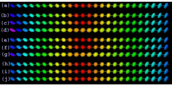
and Σ2= 4Σ1.The simulated SPD matrix data is shown in Figure 2.1 (a).

2. Log normal noise model: it assume that log(Si) has a symmetric matrix variate normal

distri-butionN(0,Σ) (see Schwartzman (2006)). Thus we simulatedi from N(0,Σ) and then calculated Si = exp(log(D(xi)) +i). The simulated SPD matrix data is shown in Figure 2.1 (b).

3. Rician noise model: this noise model is commonly assumed in DT-MRI studies. The

diffusion-weighted MR signal was simulated for 31 gradient directions rk, k = 1,· · ·,31 with b-factor bk =

(38)

considered. We set the baseline signal intensity w0 at 1500 andσ0 = 75 to obtain a signal-to-noise ratio 25. For a given diffusion tensor D(xi), we add complex Gaussian noise having a standard

deviation σ0 to the simulated real signal w0exp(−bkrkD(xi)rk) at the k-th acquisition. i.e. we

calculated

wi,k =

q

(w0exp(−bkrkD(xi)rk) +1,k)2+2₂_,k

where1,k and2,k were generated from a Gaussian random generator with mean zero and standard

deviationσ0as the resulting diffusion weighted MR signal at thek-th acquisition. Then the diffusion tensorSiwas estimated from the 35 diffusion-weighted images by applying a least squares technique

to the log-transformed signal intensities. The simulated DT (SPD matrix) data is shown in Figure

2.1 (c).

We set n = 50 and then simulated 100 data sets for each case. For each simulated dataset {(xi, Si) : i = 1,· · · , n}, we apply our methods and also the local constant and linear methods

under the Euclidean metric to estimate the SPD matrix function and the bandwidth was chosen

separately for each estimator using its corresponding cross-validation method.

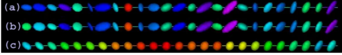
Figure 2.2 displays the estimated SPD using local linear regression under the affine invariant,

Log-Euclidean and Euclidean metrics for the three different noise models. Note that three

smooth-ing methods did an excellent job of recoversmooth-ing ground truth for the Rician noise model. For the

other two noise models, our intrinsic local linear regression methods outperform that using the Euclidean metric. There is a clear swelling effect when using Euclidean smoothing method.

Figure 2.1: Ellipsoidal representations of the simulated SPD matrix data along the design points under the three different noise models: (a) Riemannian log normal, (b) log normal and (c) Rician noise models, colored with FA values defined in (2.5.1).

2.5.1 Simulation 1

(39)

Figure 2.2: Ellipsoidal representations of the true (a) and estimated SPD matrix data along the design points using three smoothing methods: ((b), (e) and (h)) ILPR under the affine invariant metric, ((c), (f) and (i)) ILPR under the Log-Euclidean metric and ((d), (g) and (j)) LPR under the Euclidean metric and under the three different noise models: (b)-(d) Riemannian log normal, (e)-(g) log normal and (h)-(j) Rician noise models, colored with FA values defined in (2.5.1).

Euclidean metric and tensor spline method in Barmpoutis et al. (2007), respectively. For each

simulated dataset, an Average (over the design points, xi, for i = 1,· · · , n) Geodesic Distance

(AGD) across all pairs of the estimated and true SPD matrices ˆD(xi) andD(xi) was calculated as

AGDj =n−1 n

X

i=1

g(103Dˆj(xi),103D(xi)).

At each sample point xi, a Local Average (over simulated realizations, j = 1,· · · , N) Geodesic

Distance (LAGD) was calculated as

LAGD(xi) =N−1 N

X

j=1

g(103Dˆj(xi),103D(xi)),

where ˆDj(xi) are the estimated SPD matrices at the sample point xi at the j-th replication. We

take three different metrics for calculating the geodesic distance: affine invariant, Log-Euclidean

and Euclidean metrics. Results for the three different noise models are summarized in Figure 2.3

and Figure 2.4.

(40)

LCL LLL LCR LLR SP LCE LLE 0 0.2 0.4 0.6 0.8 1 1.2 AGD (a)

LCL LLL LCR LLR SP LCE LLE 0 0.2 0.4 0.6 0.8 1 1.2 AGD (b)

LCL LLL LCR LLR SP LCE LLE 0 0.2 0.4 0.6 0.8 1 1.2 AGD (c)

LCL LLL LCR LLR SP LCE LLE 0 0.2 0.4 0.6 0.8 1 1.2 AGD (d)

LCL LLL LCR LLR SP LCE LLE 0 0.2 0.4 0.6 0.8 1 1.2 AGD (e)

LCL LLL LCR LLR SP LCE LLE 0 0.2 0.4 0.6 0.8 1 1.2 AGD (f)

LCL LLL LCR LLR SP LCE LLE 0 0.05 0.1 0.15 0.2 AGD (g)

LCL LLL LCR LLR SP LCE LLE 0 0.05 0.1 0.15 0.2 AGD (h)

LCL LLL LCR LLR SP LCE LLE 0 0.05 0.1 0.15 0.2 AGD (i)

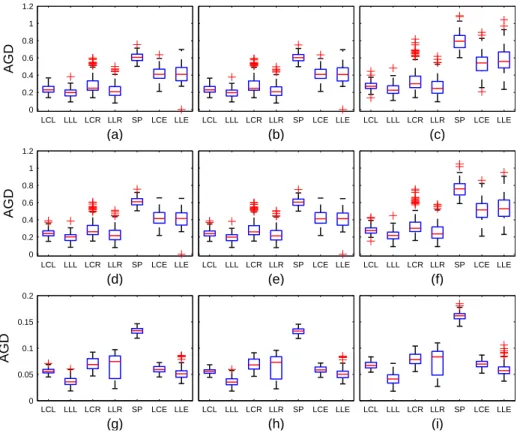
Figure 2.3: Boxplots of the AGD using the intrinsic local constant and linear estimators under the Log-Euclidean, affine invariant and Euclidean metrics, and tensor spline smoothing method, based on 100 replications for the three noise models: (a)-(c) Riemannian log normal, (d)-(f) log normal, and (g)-(i) Rician at sample size 50. The first, second and third columns correspond to comparisons based on geodesic distances under the affine invariant, Log-Euclidean and Euclidean metrics. LCL, LLL, LCR, LLR, LCE, LLE and SP represent the intrinsic local constant and linear estimators under the Log-Euclidean, affine invariant and Euclidean metrics and tensor spline smoothing method, respectively.

similar results. In addition, as expected, under each of three metrics considered, the local linear

estimator is superior to the local constant estimator. Also, our intrinsic estimators perform better

than the local constant and linear estimators under the Euclidean metric and the tensor spline

method for the first two noise models. For the third noise model, our intrinsic local estimator

under the Log-Euclidean metric works best. The second one is the estimator under the Euclidean

metric. The third one is that under the affine invariant metric. It appears that the tensor spline method cannot compete with the other six methods. Moreover, it is observed that the variances of

the AGD’s based on the affine invariant metric are larger than those based on the Log-Euclidean

metric. This suggests that the Log-Euclidean metric may be more useful. More can be observed