RATIONAL HOMOLOGY DISK SMOOTHING COMPONENTS OF WEIGHTED HOMOGENEOUS SURFACE SINGULARITIES
Jacob R. Fowler
A dissertation submitted to the faculty at the University of North Carolina at Chapel Hill in partial fulfillment of the requirements for the degree of Doctor of Philosophy in the Department of
Mathematics.
Chapel Hill 2013
c
2013
ABSTRACT
Jacob R. Fowler: Rational homology disk smoothing components of weighted homogeneous surface singularities
(Under the direction of Jonathan Wahl)
Recent work by Bhupal, Stipsicz, Szab´o, and Wahl has resulted in a complete list of the resolution graphs of weighted homogeneous complex surface singularities which admit smoothings with vanishing Milnor number; i.e., the Milnor fiber is a rational homology disk (“QHD”). There are nine families of star-shaped graphs, with central node of valency 3 or 4. Our goal is to describe all theQHD-smoothing components in the base space of the semiuniversal deformation of such a singularity. For many of the singularities (including all valency 4 examples) we show that either there is a unique such smoothing component, or there are two, related by complex conjugation or by an automorphism of the singularity. However, in the latter case we show there is a unique QHD Milnor fiber, up to diffeomorphism.
To Poppa.
ACKNOWLEDGMENTS
I would like to thank the mathematics community at the University of North Carolina at Chapel Hill. In particular, I appreciate the useful questions and conversations with my committee members: Prakash Belkale, Jim Damon, Shrawan Kumar, and Rich´ard Rim´anyi. I am especially grateful to my advisor, Jon Wahl, for his incredible guidance, patience, and support. I would also like to give thanks to my fellow graduate students, especially Alex, Amanda, Ryan, Brandyn, and Michael. They have not only provided me with numerous interesting mathematical discussions, but they are also great friends.
TABLE OF CONTENTS
List of Figures . . . ix
List of Tables . . . x
Introduction . . . 1
Chapter 1. Preliminaries . . . 12
1.1 Lattices and discriminant forms . . . 12
1.1.1 Overlattices . . . 12
1.1.2 Embeddings into unimodular lattices . . . 13
1.2 The linking pairing for a rational homology 3-sphere . . . 13
1.3 Normal surface singularities withQHS links . . . 14
1.3.1 The discriminant group . . . 14
1.3.2 Other invariants . . . 15
1.4 Smoothings of surface singularities . . . 16
1.4.1 The isotropic subgroup of a smoothing . . . 16
Chapter 2. Smoothings of negative weight . . . 18
2.1 Normal surface singularities withC∗-action . . . 18
2.1.1 Compactifications ofX . . . 19
2.1.2 The dual graph . . . 20
2.2 Deformations of negative weight . . . 21
2.2.1 Relative compactifications . . . 21
2.2.2 Marked surfaces associated toX . . . 22
2.3 Smoothings of negative weight withµ= 0 . . . 26
2.3.1 Smoothing components . . . 26
2.3.2 Self-isotropic subgroups . . . 27
Chapter 3. The model surfaces . . . 29
3.1 Γ-surfaces . . . 29
3.1.1 Self-isotropic subgroups . . . 29
3.2 Model Γ-surfaces and basic self-isotropic subgroups . . . 31
3.2.1 Automorphisms and Γ-surfaces . . . 31
3.2.2 Complex conjugation . . . 32
3.3 Uniqueness of the models . . . 33
3.3.1 Proofs of the main theorems . . . 33
3.3.2 Outline of the constructions and proof of uniqueness . . . 34
3.4 The geometry of Γ-surfaces . . . 36
3.4.1 The canonical divisor . . . 36
3.4.2 Irreducible curves . . . 37
3.4.3 Divisors and irreducible (−1)-curves . . . 38
3.5 Construction and uniqueness of the model surfaces . . . 41
3.5.1 FamilyW . . . 42
3.5.2 FamilyN . . . 47
3.5.3 FamilyM . . . 51
3.5.4 FamilyA4 . . . . 56
3.5.5 FamilyB4 . . . . 66
3.5.6 FamilyC4 . . . . 74
3.5.7 FamilyB3 2 . . . 86
3.5.8 FamilyC3 2 . . . 92
3.5.9 FamilyC3 3 . . . 96
Chapter 4. Impermissible self-isotropic subgroups . . . 101
4.1.2 Example: W(3,3,3) . . . 104
4.2 Impermissibility and Pinkham’s method . . . 107
4.2.1 Example: M(2,0,1) . . . 107
Appendix A. The graphs and their dual graphs . . . 112
Appendix B. Tables of discriminant groups . . . 118
LIST OF FIGURES
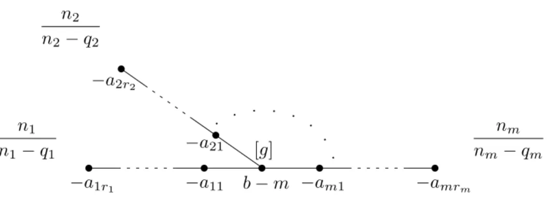
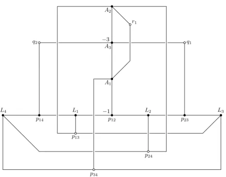
2.1 The resolution graph of a weighted homogeneous singularity. . . 19
2.2 The dual graph of a weighted homogeneous singularity. . . 20
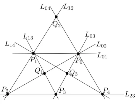
3.1 A4—The initial configuration of points and lines . . . . 57
3.2 A4—Additional points and lines are added . . . . 57
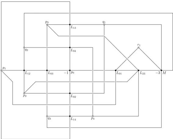
3.3 A4—The final plane curve configuration . . . . 58
3.4 A4—The configuration of curves on ˜Z . . . . 60
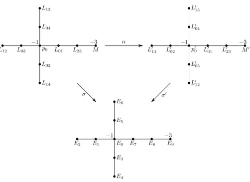
3.5 A4—Two Γ-surfaces related by an automorphism of the graph . . . . 62
3.6 The M¨obius-Kantor configuration . . . 63
3.7 B4—Construction of the plane curve . . . . 67
3.8 B4—The final plane curve configuration . . . . 67
3.9 B4—The configuration of curves after blowing up. . . . . 69
3.10 C4—Initial configuration of lines . . . . 75
3.11 C4—Additional lines are added . . . . 76
3.12 C4—The final plane curve configuration . . . . 78
3.13 C4—The configuration of curves on ˜Z . . . . 79
3.14 C4—The configuration of curves on ˜Z, including the additional curveg 1 . . . 80
3.15 B3 2—Construction of the plane curve . . . 87
3.16 B3 2—The configuration of curves after blowing up . . . 87
3.17 C3 2—The configuration of curves after blowing up. . . 92
3.18 C3 3—Construction of the plane curve . . . 97
3.19 C3 3—The configuration of curves after blowing up. . . 97
LIST OF TABLES
3.1 Symmetries of the dual graphs . . . 32
4.1 W(3,3,3)—The invariants for the action of I1. . . 106
4.2 W(3,3,3)—The invariants for the action of I3 orI4. . . 107
A.1 The resolution graphs of the singularities . . . 113
A.2 The dual graphs of the singularities . . . 115
B.1 Discriminant groups for the six exceptional families . . . 119
B.2 Discriminant groups for familyW . . . 120
B.3 Discriminant groups for familyN . . . 123
INTRODUCTION
Let X={f(x, y, z) = 0} ⊂C3 be a surface with an isolated singular point at the origin. We will consider the behavior of X in a small neighborhood B(0) of the singular point. The link of the singularity at 0 is the smooth 3-manifoldL=X∩∂B¯ (0). In his classic book [15], Milnor studied the properties of a “nearby smooth fiber”M =f−1(t)∩B¯(0), where 0<|t| . M is a smooth 4-manifold with boundaryL, called the Milnor fiber ofX. Milnor showed thatM has the homotopy type of a bouquet of 2-spheres, the number of which is the Milnor number µ:= rkH2(M,Z). µ may be calculated as the colength of the Jacobian ideal off, and is an important invariant of the singularity.
Now consider an arbitrary germ (X,0) of a normal surface singularity, not necessarily a hypersur-face or complete intersection. Following Wahl [37], one can again consider “nearby smooth fibers” by studying smoothings of the singularity. Asmoothing of (X,0) is a flat morphism f : (X,0)→(C,0), where (X,0) is a germ of an isolated three-dimensional singularity, together with an identification
i: (X,0)−→∼ (f−1(0),0). TheMilnor fiber of the smoothing isM =f−1(t)∩B¯(0) (where ¯B(0) is a ball in some CN containingX). M is a smooth 4-manifold whose boundary is the link Lof the singularity (X,0). It has the homotopy type of a finite CW-complex of dimension 2, with first Betti number b1(M) = 0 [8]. We define theMilnor number of the smoothing to be µ= rkH2(M,Z).
Unlike in the case of a hypersurface or complete intersection,µandM are not generally invariants of the singularity (X,0). One might have different smoothings of the same singularity with distinct Milnor fibers, and even different Milnor numbers. The first example of this phenomenon, due to Pinkham [27], occurs when X is the cone over the rational normal curve of degree 4. For this singularity there are two distinct Milnor fibers, one with µ= 1 and the other withµ= 0.
[13]) and unpublished (but known to the experts—see e.g. [32, p. 123], [4, p. 505]), was compiled over the years by Wahl. For instance, in [13] it is shown that the cyclic quotient singularities which admitQHD-smoothings are exactly those of type p2/(pq−1), wherep > q >0, and (p, q) = 1. The example of Pinkham’s is the special case where p= 2,q= 1. Recall that the resolution graph of such a singularity is a chain of rational curves with self-intersections given by the Hirzebruch-Jung continued fraction of p2/(pq−1); the set these graphs will be called G. Aside from these cyclic quotients, all the examples on Wahl’s list havestar-shaped resolution graphs—i.e. the graph contains exactly one vertex with valency>2.
Recent interest in QHD-smoothings has been sparked by an application to differential topology, via the rational blow-down of Fintushel and Stern [7] (generalized by Park [24]). The familiar blow-up operation in algebraic geometry replaces a point on a surface with a curve of self-intersection
−1. The inverse operation is called the blow-down. From a differential topological point of view, blowing down can be thought of as a surgery operation on smooth 4-manifolds, removing a tubular neighborhood of a 2-sphere (with self-intersection−1) and pasting in a 4-disk. In the (generalized) rational blow-down, one removes an appropriate tubular neighborhood of a chain of 2-spheres with self-intersections given by the Hirzebruch-Jung continued fraction ofp2/(pq−1) (p > q >0 relatively prime), and pastes in the rational homology disk Milnor fiberM. The natural Stein structure on
M leads to the formula of [7] relating the Seiberg-Witten invariants of the resulting 4-manifold with those of the original (though this interpretation came later—see [34]). This procedure has been applied to find exotic smooth structures on some familiar 4-manifolds (see e.g. [25], [26], [33], [14]).
needed.
Additionally, the examples of QHD-smoothings on Wahl’s list were presented in [34] for the first time, and were organized into these families (with two exceptions, which were nonetheless known to the authors of [34] and would appear subsequently in [1]). Two different techniques of construction were used. The technique used in [34, Section 8.1] (and later in [1]) applies Pinkham’s theory of “smoothings of negative weight” [27][29]. In this construction the Milnor fiber arises as the complement of a curve on a rational surface. In the “quotient construction,” theµ= 0 smoothing is a quotient of a smoothing of a familiar hypersurface or complete intersection singularity. This technique was used to constructQHD-smoothings for familiesW,N,A4, and B4 in [34, Section 8.2], and later for C4 in [38].
Follow-up work by Bhupal and Stipsicz [1] showed that the old list of examples gives a complete list of all star-shaped graphs that admitQHD-smoothing. They are labeled as follows: there are three 3-parameter familiesW,N, andM, with central node of valency 3; three 1-parameter families
A4,B4, andC4, with central node of valency 4; and three “exceptional” 1-parameter familiesB3 2,
C3
2, andC33 with central node of valency 3. (The upper index indicates the valency of the central node; for an explanation of the lower index, see [1]. There are also star-shaped familiesA3, B3
4, and
C3
6 that admit QHD-smoothing, but these are already contained inM.) We give the complete list of these graphs in Table A.1 in the appendix. We summarize the preceding results in the following
Theorem 1 (Bhupal–Stipsicz–Szab´o–Wahl). LetΓ¯ be a star-shaped graph. Then Γ¯ admitsQ HD-smoothing if and only if Γ¯∈ W ∪ N ∪ M ∪ B3
2∪ C32∪ C33∪ A4∪ B4∪ C4.
Wahl has conjectured [38] that there are no non-star-shaped graphs that admit QHD-smoothing. This would imply that the graphs listed in Theorem 1, together with the setG of the graphs of the cyclic quotient singularities of typep2/(pq−1), are the only graphs that admit
QHD-smoothing. Park, Shin, and Stipsicz [23] have recently asserted a proof of this conjecture.
particularly important consequence of this is that all these singularities are weighted homogeneous (also called quasi-homogeneous, or singularities with good C∗-action), and the QHD-smoothings are smoothings of negative weight. (These terms are defined in Chapter 2.)
Our primary goal in this paper is to describe all QHD-smoothings for each normal surface singularity (X,0) whose resolution graph is listed in Theorem 1. More precisely, we want to describe the part of the semiuniversal deformation space on which the QHD-smoothings occur. Let
ρ : (V,0) → (B,0) denote the semiuniversal deformation of (X,0). The base space decomposes into irreducible components B =S
Bi. A component Bi is called a smoothing component if the
general fiber overBi is smooth. By versality any smoothing of (X,0) arises as a pullback from a
unique smoothing component. The Milnor fiber and Milnor number are invariants of the smoothing component.
Wahl has shown that a QHD-smoothing component for a weighted homogeneous singularity must have dimension 1 [38, Theorem 2]. So our primary problem is to enumerate the smoothing components and describe their Milnor fibers. To state our main result we will need some preliminary notions (careful definitions will be given in Chapter 1).
Associated to a negative-definite weighted graph ¯Γ is its discriminant group D(¯Γ), which we define in Section 1.3.1. D(¯Γ) is a finite abelian group with a natural pairingD(¯Γ)×D(¯Γ)→Q/Z. When ¯Γ is the resolution graph of a singularity X withQHS linkL,D(¯Γ) is naturally isomorphic to H1(L,Z) with its torsion linking pairing. In [13], Looijenga and Wahl associate an isotropic subgroup I ⊂D(¯Γ) to every smoothing component of X. If we denote byM the Milnor fiber of the smoothing, thenI is determined by the topology of the inclusion L=∂M ⊂M (see Section 1.4.1). For the case of a smoothing withQHD Milnor fiberM, |D(¯Γ)|is a square and I and isself-isotropic under the linking pairing. In this caseI is the kernel of the natural surjectionH1(L,Z)→H1(M,Z).
In fact, [13] associates to each smoothing component ofX a collection of algebraic invariants, called a “set of smoothing data ofX”, one of which is the previously mentioned isotropic subgroup. This is organized (at least for Gorenstein X) into a map Sm(X) → S(X) from the set Sm(X) of smoothing components of X to the set S(X) of possible sets of smoothing data forX. Following their example, we can summarize the discussion of the self-isotropic subgroup as follows. Fix a graph ¯
subgroups I ⊂D(¯Γ). Then there is a natural map
ξ : Sm0(X)→ I(¯Γ)
taking aQHD-smoothing component to its associated self-isotropic subgroupI ⊂D(¯Γ).
We will describe the set of QHD-smoothing components of X by studying the image and fibers of this map. It turns out that ξ is surjective, except for some graphs inW,N, andM. However, in all cases there are certain known elements in the image of ξ, which we callbasic self-isotropic subgroups. These are defined in Chapter 3; they are the self-isotropic subgroups associated to certain carefully constructed “model” smoothings (see in particular Section 3.2). For a given graph ¯
Γ, there will be either one or two basic self-isotropic subgroups:
(a) For ¯Γ∈ W with p=q =r, ¯Γ∈ M with p=r+ 1, or ¯Γ∈ A4, there are two basic self-isotropic subgroups I ⊂D(¯Γ).
(b) For all other cases there is a unique basicI ⊂D(¯Γ).
We will restrict ourselves to studying those smoothing components that correspond to basic self-isotropic subgroups. Let B ⊂ I(¯Γ) denote the subset of basic self-isotropic subgroups, and denote byξB the restricted map
ξB:=ξ|ξ−1(B):ξ−1(B)→B.
Our main result concerns the fibers ofξB. We state it in two parts, first for the valency 3 families. Theorem 2. Let Γ¯ be a valency 3 star-shaped graph that admits QHD-smoothing, and let X be the unique singularity with resolution graph Γ. Then:¯
(a) If Γ¯ ∈ C3
2, then ξB is 2–1.
(b) In all other cases, ξB is a bijection.
As it turns out, the restriction to basic self-isotropic subgroups is not an issue in “most” cases: for the valency 3 exceptional families B3
Corollary 3. Let Γ¯ ∈ B3
2 ∪ C23∪ C33 be a valency 3 exceptional graph, and let X be the unique
singularity with resolution graph Γ. Then¯ I(¯Γ)is a singleton and ξ=ξB is surjective. So,
(a) if Γ¯ ∈ C3
2, X has two QHD-smoothing components; (b) otherwise X has a unique QHD-smoothing component.
For certain graphs in families W, N, and M, the discriminant group contains non-basic self-isotropic subgroups. A list of known examples of these is given in Appendix B. The failure ofξto be surjective in these cases is studied in Chapter 4. There we show that in certain particular examples, the non-basic I are impermissible—they cannot correspond to anyQHD-smoothing component. This provides evidence for a
Conjecture 4. If I ⊂D(¯Γ)is a non-basic self-isotropic subgroup, then I is impermissible.
If true, then for graphs in familiesW,N, andMthe image ofξwould be exactlyB. This would imply thatξ =ξB, and so Theorem 2 would give a complete enumeration of the QHD-smoothing components for these cases as well.
Now we turn to the valency 4 graphs, where the issue of the cross-ratio on the central curve creates additional subtlety. Fix a valency 4 graph ¯Γ, and for λ ∈ C− {0,1} let Xλ denote the
singularity with resolution graph ¯Γ and cross-ratio λ. Recall that two cross-ratios λ, λ0 ∈C− {0,1}
are equivalent if they are identified under the action ofS3 generated by λ7→1/λandλ7→1−λ. In this case Xλ and Xλ0 are analytically equivalent singularities.
Denote
ξλ : Sm0(Xλ)→ I(¯Γ)
the map taking aQHD-smoothing component of Xλ to its associated self-isotropic subgroup. For
the valency 4 families (as with the valency 3 exceptional families), all self-isotropic subgroups are basic; i.e., B=I(¯Γ). So there is no need to restrict to the basic self-isotropic subgroups to state our main result for the valency 4 graphs:
Theorem 5. Let Γ¯ be a valency 4 star-shaped graph that admits QHD-smoothing. Then: (a) There is a unique cross-ratio λfor which Sm0(Xλ) is nonempty:
(ii) harmonic (λ=−1, 1/2, or 2), forΓ¯ ∈ B4;
(iii) λ= 9 (or1/9, −8, −1/8, 9/8, or 8/9), for Γ¯∈ C4.
(b) For this particular cross-ratio λ, the map ξλ is surjective and
(i) 2–1 ifΓ¯ is in B4, or if Γ¯ is in C4 with parameter p≥1; (ii) 1–1 ifΓ¯ ∈ A4, or if Γ¯ is the graph in C4 with p= 0.
Remark. It was previously known (as a consequence of [38, Theorem 2]) that there are only finitely many cross-ratios for which QHD-smoothings could occur. The quotient constructions provided in [38] for these graphs produced QHD-smoothings for only one cross-ratio in each case. Theorem 5(a) states that indeed these are the only possibilities. Combined with Theorem 1 (and the fact that the valency 3 graphs are taut), this result gives a complete list of all weighted homogeneous singularities that admit QHD-smoothing.
As a consequence of Theorem 5, we can completely enumerate the QHD-smoothing components for the valency 4 graphs:
Corollary 6. Let Γ¯∈ A4∪ B4∪ C4 be a valency 4 graph, and let λ be the appropriate cross-ratio listed in Theorem 5(a). Then,
(a) if Γ¯ is the graph in C4 with parameterp= 0, then X
λ has one QHD-smoothing component; (b) otherwise Xλ has two QHD-smoothing components.
The proofs of the main theorems are performed using a uniform technique, which has two main steps. The first step (Chapter 2) is to establish a 1–1 correspondence between QHD-smoothing components and certain rational surfaces that contain marked curve configurations, up to an appropriate notion of identification. Then the second step (Chapter 3), which is the main part of the problem and the bulk of the work, is to describe explicitly the construction of these surfaces and prove that they are unique. We summarize our technique below.
weight of X extends to a deformation of a natural compactification of X, whose general fiber Z
is a “compactified Milnor fiber”. The compactification of X is obtained by adding a (reducible) curveE∞ at infinity, which is configured by the dual graph Γ of ¯Γ (defined in Section 2.1.2). The deformation is trivial nearE∞, so this curve also sits on the surfaceZ; to be precise, one obtains a curveE =S
Ei ⊂Z with an identification σ:E −→∼ E∞. The Milnor fiber is then diffeomorphic toZ−E. In order for the Milnor fiber to be aQHD,Z must be rational and the curves Ei must span the rational homologyH2(Z,Q). We call a triple of data (Z, E, σ) a “Γ-marked surface,” or “Γ-surface.”
A key theorem of Pinkham ([29, Theorem 6.7], stated in this paper as Theorem 2.2.3) provides a partial converse: given appropriate data (Z, E, σ) as above, one can construct a smoothing of
X whose compactified Milnor fiber is Z. In Section 2.3 we use this theorem to establish a 1–1 correspondence between QHD-smoothing components and Γ-marked surfaces, taking great care to establish the appropriate notion of isomorphism of Γ-surfaces. The associated self-isotropic subgroup I ⊂D(¯Γ) has an interpretation under this correspondence: it determines the embedding
H2(E,Z),→H2(Z,Z), or equivalently the embeddingLZ[Ei],→PicZ.
In Chapter 4 we undertake the task of classifying the Γ-marked surfaces. For each graph ¯Γ, we first construct the “model” Γ-surfaces, which correspond to the previously known smoothing components. The basic self-isotropic subgroups are defined to be those associated to the models. These are listed carefully in Section 3.2. The main results then follow from the following
Theorem(3.3.1). Suppose(Z, E, σ)is aΓ-surface whose associated self-isotropic subgroupI ⊂D(Γ) is basic. Then (Z, E, σ) is isomorphic to one of the corresponding models.
The model Γ-surfaces are constructed by blowing up certain specially constructed plane curves
general techniques developed in Section 3.4. After we blow down these curves, the result follows from the observation that the resulting plane curve is unique; the curves used in our constructions are carefully chosen to ensure that this is evident.
For the valency 4 graphs A4,B4, andC4, the curves used in the constructions of the models (in Sections 3.5.4, 3.5.5, and 3.5.6 respectively) force a particular cross-ratio on the central curve of the dual configuration E. This fact, together with the uniqueness of the models, is used to prove Theorem 5(a).
In [34, Section 8.1], smoothings for graphs in familiesW andN were constructed by blowing up four lines in general position in the plane. This has the consequence that the fundamental group of the Milnor fiber is abelian. Our model surfaces for these cases are constructed in the exact same way. For graphs in family M, we have also been able to construct our model surface by blowing up 4 lines in general position (see Section 3.5.3). Our construction may be seen as a new construction of the surface that was constructed in [34, Example 8.3], and allows us to conclude that π1(M) is abelian for this case as well:
Theorem 7. Let Γ¯ ∈ M, and let X be the unique singularity with graph Γ. Suppose¯ M is the Milnor fiber of aQHD-smoothing of X whose associated I ⊂D(¯Γ)is basic; then π1(M) is abelian (and hence isomorphic to I).
Remark. Alternatively, for familiesW andN one could see that π1(M) is abelian from the quotient constructions of [34, Section 8.2], whereM is obtained as the quotient of a simply connected space by a finite abelian group. However, there is no known quotient construction for graphs inM(and indeed, there are reasons to believe that such a construction is not possible). For a smoothing of a singularity whose graph is in A4,B4, orC4, the quotient constructions of [38] imply thatπ
1(M) is a nonabelian metacyclic group. The problem of computing π1(M) for the exceptional valency 3 families B3
2,C23, andC33 remains open.
In all cases where there are two model surfaces, they are closely related to each other. For familiesC3
the graph—the two models differ only in the way the marked curve is identified with the graph. In these cases, the corresponding smoothing components correspond to distinct self-isotropic subgroups of D(¯Γ), but have isomorphic total spaces; the identification of the special fiber with the original singularity differs by an automorphism of the singularity. This is discussed in Section 3.2.1.
The case of A4 is particularly interesting. In this case there are two models that are related by complex conjugation. However, they correspond to distinct self-isotropic subgroups. The two model surfaces are related by an automorphism of the dual graph that is not induced by an automorphism of the underlying curve configuration. This subtlety is a consequence of the special cross-ratio of the points on the central curve, and is discussed in detail in Section 3.5.4. The existence of two smoothing components in this case had previously been discovered by Wahl [38], using a quotient construction. In his construction the total spaces of the smoothings arise as quotients ofC3 by two different subgroups of GL(3,C) which are not conjugate in GL(3,C), but are conjugate as subgroups of GL(6,R). The preceding observations lead to the following result.
Theorem 8. Let Γ¯ be a star-shaped graph that admits QHD-smoothing. If the only self-isotropic subgroups of D(¯Γ) are basic or impermissible, then the QHD Milnor fiber is unique up to diffeomor-phism.
We note that while the Milnor fiber is unique up to diffeomorphism, the diffeomorphism may not preserve the orientation. This may occur in the cases where the smoothings are related by complex conjugation. (See also Remark 3.5.9.)
Remarks. This work, as well as [34], [1], and [38] preceding it, can be viewed in the context of a broader problem: the link L of a normal surface singularity X has a natural contact structure, and one may wish to classify the possible symplectic fillings ofL. Of course, the Milnor fiber of a smoothing of X has a natural Stein (and hence symplectic) structure, and so provides a possible example of such a filling. In fact, [1] proves a stronger result than Theorem 1: the graphs listed there are the only graphs of weighted homogeneous normal surface singularities whose links can admit a symplectic filling by a rational homology disk. While our Theorem 8 provides a restriction on the possible QHD Milnor fibers that can occur, we do not rule out the possibility that other QHD symplectic fillings might arise from different methods.
CHAPTER 1
Preliminaries
1.1 Lattices and discriminant forms
In this section we develop the theory of lattices and their discriminant forms, following [19] and [13,
§1]. A lattice is a free abelian groupLtogether with a nondegenerate integral symmetric bilinear form·:L×L→Z. A morphism of lattices φ:L1 →L2 is a morphism of abelian groups such that
φ(x)·φ(y) =x·y. Given a choice of basis ofL, the bilinear form may be represented as a matrix
B. The assumption that the form is nondegenerate is equivalent to detB6= 0. Lis unimodular if detB =±1.
Theadjoint homomorphism is the morphism of abelian groups ad :L→L∗ = HomZ(L,Z) given byx7→(x· −). The form is nondegenerate (resp. unimodular) if and only if ad is an injection (resp. isomorphism).
By inverting the matrix B we obtain an injectionL∗,→L⊗ZQwhose image is
{x∈L⊗ZQ|x·y∈Z, ∀y∈L}.
The bilinear form onLthus extends to a bilinear formL∗×L∗ →Qwhich is integral when restricted to L⊂L∗. The discriminant group of L is the finite abelian group D=L∗/L. The form on L∗
descends to a bilinear form b:D×D→Q/Zcalled the discriminant bilinear form of L.
1.1.1 Overlattices
An overlattice of L is an embedding i:L ,→M of lattices of the same rank. (This occurs if and only if M/Lis finite.) Two overlattices i1 :L ,→M1 and i2 :L ,→M2 of Lareisomorphic if there is an isomorphism φ:M1
∼
For a given overlattice i : L ,→ M, the adjoint homomorphism L ,→ L∗ decomposes as a compositionL ,→M ,→M∗ ,→L∗, whereM ,→M∗ is the adjoint homomorphism ofM. This gives rise to a subgroup I =M/L⊂L∗/L=Dwhich is isotropic sinceI ⊂I⊥=M∗/L. Conversely, any isotropic subgroup ofD arises from an overlattice ofL, and two overlattices are isomorphic if and only if they correspond to the sameI ⊂D[19, 1.4.1].
1.1.2 Embeddings into unimodular lattices
Let U be a unimodular lattice, and let L1 ⊂U be a primitive sublattice (i.e. U/L1 is free). Let
L2 =L⊥1 ⊂U. Let (D1, b1) and (D2, b2) be the corresponding discriminant bilinear forms. Then there is a natural isomorphism of groups α :D1
∼
−→D2 such thatb1(x, y) =−b2(α(x), α(y)) [19, 1.6.1]. We say that α is ananti-isomorphism of the discriminant bilinear forms.
Conversely, if L1 andL2 are any two lattices and there is an anti-isomorphism α:D1
∼
−→D2, then there naturally exists a unimodular overlattice U with L1, L2 ⊂U primitive and L2 =L⊥1.
1.2 The linking pairing for a rational homology 3-sphere
Let Lbe a smooth compact 3-manifold that is a rational homology sphere, orQHS; this means that
H1(L,Q) = 0. (Note that in this caseHi(L,Q)'Hi(S3,Q), whereS3 is the 3-sphere.) Then there is a natural pairing
`:H1(L,Z)×H1(L,Z)→Q/Z
called thelinking pairing ortorsion linking form ofL. `(x, y) is defined as follows: representx= [X] and y= [Y] where X and Y are 1-chains. Then, sincex is torsion there exists an nso that nX is the boundary of a 2-chain Z. Then
`(x, y) = 1
nhZ, Yi modZ
where hZ, Yi is the transverse intersection number ofZ and Y.
` is a nondegenerate symmetric pairing since its adjoint H1(L,Z) → HomZ(H1(L,Z),Q/Z), taking x 7→ `(x,·), is an isomorphism of groups. This is a consequence of Poincar´e duality
H2(L,Z)'Hom(H1(L,Z),Q/Z).
Remark 1.2.1. In fact, the torsion linking form is defined for an arbitrary smooth compact manifold
M of dimensionn. In this case we have pairings
Hi(M,Z)t×Hn−i−1(M,Z)t→Q/Z
where the tsubscript indicates the torsion part of the group.
1.3 Normal surface singularities with QHS links
Let (X,0) be a germ of a normal surface singularity. IfX1 ⊂CN is a representative of the germ and ¯Bε(0) is a sufficiently small closed ball about 0, thenX :=X1∩B¯ε(0) is contractible and is
homeomorphic to the cone over its boundaryL:=X∩∂Bε¯ (0). The smooth compact 3-manifold
L is called the link of the singularity. X is a surface with boundary ∂X = L, and is a “good representative” of the germ. We will assume for the rest of this section thatLis a rational homology sphere.
Denote by π : ˜X → X the minimal good resolution of X, with exceptional configuration
E := π−1(0) = Sn
i=1Ei. (Recall that the resolution is “good” if each Ei is smooth, and the
intersections Ei∩Ej are simple normal crossings with no triple intersections.) ˜X is a nonsingular
complex manifold with boundary∂X˜ =L. Lis aQHS if and only ifE is a tree of rational curves. Let ¯Γ denote the resolution dual graph, i.e. the dual graph of the curveE. ¯Γ is a weighted graph with a vertex vi corresponding to each curve Ei, and edges and weights determined by the intersection numbersEi·Ej.
1.3.1 The discriminant group
The resolution ˜Xdeformation retracts ontoE, which is a tree of rational curves. SoHi( ˜X)'Hi(E) is free of rank 1,0, nfor i= 0,1,2 respectively. Let
E(¯Γ) := M
be the lattice with pairing given by the weighted graph ¯Γ. The intersection pairing on H2( ˜X) is given by ¯Γ, and so there is a natural isomorphism of lattices H2( ˜X)'E(¯Γ).
The long exact sequence of the pair ( ˜X, L) gives
H2(L) 0 //H2( ˜X)
j //
H2( ˜X, L) ∂ //H1(L) //H1( ˜X) = 0
where H2(L) is torsion andH2( ˜X)'E(¯Γ) is free, so the first map is≡0. FurthermoreH2( ˜X, L)'
H2( ˜X)'HomZ(H2( ˜X),Z)'E(¯Γ)∗ by Lefschetz duality and the universal coefficient theorem, and the map j is the adjoint of the intersection pairing. So we may rewrite this as
0 //E(¯Γ) ad //E(¯Γ)∗ //H1(L) //0.
(This is essentially the description ofH1(L) given by Mumford in [16].) Thus we have an isomorphism of the discriminant group D(¯Γ) := E(¯Γ)∗/E(¯Γ) 'H1(L), and the discriminant form onD(¯Γ) is equal to the linking pairing onH1(L) [13, 4.1.1]. The groupD(¯Γ)'H1(L) with the linking pairing will be called the discriminant group of the singularity (X,0); it is computable from the graph ¯Γ. Remark 1.3.1. One of the main results of [13] is that whenLis the link of a surface singularity (X,0), the linking pairing on L is induced by a finer object: a quadratic functionq :H1(L)→Q/Z. (A homomorphism of abelian groupsq:G→H is called aquadratic function if the mapb:G×G→H
defined by b(x, y) :=q(x+y)−q(x)−q(y) is bilinear.) The definition ofq depends in a subtle way on how the complex structure of the resolution ˜X interacts with its boundary L (see Theorem 3.7 and §4 of [13]).
1.3.2 Other invariants
We now discuss two other invariants of (X,0) that are of interest. The first is the relative canonical cohomology class K = KX˜ ∈ H2( ˜X) ' E(¯Γ)∗. K may be written as a rational combination
K =P
qiEi, qi ∈Q, by solving the adjunction equationsK·Ei+Ei·Ei=−2 for the unknownsqi.
from ¯Γ by the conditionZ·(Z+KX˜) =−2 whereZ is the fundamental cycle on ˜X(i.e. the smallest effective cycle with Z·Ei ≤0 for alli).
1.4 Smoothings of surface singularities
Recall from the introduction that a smoothing of (X,0) is a flat morphism f : (X,0) → (C,0), where (X,0) is a germ of an isolated three-dimensional singularity, together with an identification
i: (X,0)−→∼ (f−1(0),0). TheMilnor fiber of the smoothing isM =f−1(t)∩B¯(0) (where ¯B(0) is a
ball in someCN containingX, and 0<|t| ε). M is a smooth 4-manifold with boundary ∂M =L. It has the homotopy type of a finite CW-complex of dimension 2, with first Betti numberb1(M) = 0 by a theorem of Greuel and Steenbrink [8]. This impliesH2(M,Z) is free, H1(M,Z) is torsion, and
Hi(M,Z) =Hi(M,Z) = 0 for i >2. TheMilnor number of the smoothing is µ= rkH2(M,Z).
1.4.1 The isotropic subgroup of a smoothing
Let (X,0) be a singularity withQHS link L. Letf be a smoothing with Milnor fiber M, as above. The long exact sequence of the pair (M, L) gives
H2(M) //H2(M, L) ∂ //H1(L)
i∗ //
H1(M) //H1(M, L)
wherei∗ is the map induced from the inclusionL=∂M ,→M. (Here, when we omit the coefficients of homology groups, the coefficients are inZ.) H1(M, L)'H3(M) = 0 by Lefschetz duality, soi∗ is a surjection. H1(L) and H1(M) are torsion, so if we take the torsion part of the sequence we get a complex
H2(M, L)t ∂t //
H1(L)
i∗ //
H1(M) //0
which is not exact at H1(L), but im(∂t)⊂ker(i∗).
Denote I = im(∂t)⊂H1(L). Then [13, Theorem 4.5] says that I is isotropic with respect to the linking pairing onH1(L) (i.e. I ⊂I⊥), and indeedI⊥= ker(i∗). In particularH1(L)/I⊥ 'H1(M). Furthermore the discriminant bilinear form of the lattice H2(M) (with its intersection pairing) is canonically isomorphic to I⊥/I (with its bilinear pairing induced from H1(L)).
It is shown in [13, 4.13] that in fact I is an invariant of the smoothing component on which the smoothing occurs. So we may also speak of the isotropic subgroup associated to a smoothing component.
Remark 1.4.2. In fact, [13, Theorem 4.5] contains a stronger result: I is actually q-isotropic (i.e.
q|I ≡0), where q is the quadratic function of Remark 1.3.1. The intersection pairing onH2(M) is induced from the quadratic functionQM :H2(M)→Z,
QM(x) := 1
2(x·x+KM ·x),
and its “discriminant quadratic function” is isomorphic to (I⊥/I, q|I⊥).
For the case of a smoothing withµ= 0,I⊥/I is isomorphic to the discriminant group ofH2(M), which has rank 0. So we have the following
Proposition 1.4.3. For a smoothing withµ= 0, the associated isotropic subgroupI is self-isotropic, i.e. I =I⊥.
In particular this implies that I is the kernel of the surjection i∗ : H1(L) → H1(M), so
CHAPTER 2
Smoothings of negative weight
2.1 Normal surface singularities with C∗-action
Let (X, x0) be a germ of a normal surface singularity which admits an action of the multiplicative group C∗. (Note that we are no longer assuming the link is aQHS.) We will always assume theC∗ -action isgood; this means that x0 is the unique fixed point of the action. Equivalently,X = SpecA may be taken to be an affine variety where A is a nonnegatively graded ringA=L
k≥0Ak with A0 = C. In terms of equations, this means X is cut out by weighted-homogeneous equations
fi(x1, . . . , xN) = 0 (where eachxi has positive weight) in some CN; i.e.A=C[x1, . . . , xN]/I where
I = (f1, . . . , fM) is a homogeneous ideal with respect to some grading degxi =wi >0. For this reason these singularities are called weighted-homogeneous singularities.
The results of this section are due to Orlik and Wagreich [22, 20, 21] and Pinkham [28]. We will assume throughout this chapter thatX is not a cyclic quotient singularity.
Let ˜X be the minimal good resolution of X. SinceX is not a cyclic quotient, the exceptional configuration has a central curveC of genusg with self-intersection−b. Branching off fromC are m
chains of rational curvesCij whose self-intersection numbers −bij are given by the Hirzebruch-Jung continued fraction expansion
ni qi
=bi1−
1
bi2− 1 . ..−
1
bisi
.
In particular, the resolution graph ¯Γ is star-shaped (see Figure 2.1). Denote the intersection points of the arms with the central curve byPi =C∩Ci1.
Figure 2.1: The resolution graph of a weighted homogeneous singularity.
degree +b. The data consisting of the numbersni/qi, the analytic type of the curveC, the sheaf OC(D), and the points Pi ∈C uniquely determines the singularityX. Pinkham shows in [28] that the graded pieces of the ring Aare Ak=H0(C,OC(D(k))), where
D(k) =kD−X i
dkqi/niePi. (2.1)
Here dqe denotes the ceiling ofq; i.e. the least integer greater than or equal to q.
2.1.1 Compactifications of X
X has a naturalC∗-compactification ¯X, defined as ProjA[t] wheret has weight 1 with respect to the grading. Let C∞= ¯X−X= ProjA be the curve at infinity. There is a natural isomorphism
α :C −→∼ C∞ via the orbits of the C∗-action. (This may be obtained by partially resolving the singularity at x0 to obtain a surface with C∗-action containing both C and C∞.) X¯ has cyclic quotient singularities of typeni/(ni−qi) at the pointsQi =α(Pi).
Let β : ¯X0 → X¯ be the minimal resolution of these cyclic quotient singularities. LetE∞ =
β−1(C∞) = ¯X0−X be the configuration at infinity. It has a central curveE
0,∞, which is the proper
transform ofC∞. In particular, β|E0,∞ gives an isomorphism ofE0,∞ with C∞. So by composing with α we get an isomorphismγ :C −→∼ E0,∞. LetQi0 =γ(Pi). The normal bundle of E0,∞in ¯X0 is
OE0,∞(γ(D)−P
Q0i). So the self-intersection number of E0,∞ is b−m, where mis the number of arms in the resolution.
Figure 2.2: The dual graph of a weighted homogeneous singularity.
singularities. They consist of chains of rational curves Eij,∞ with self-intersections aij, given
by the continued fraction of ni/(ni −qi). The arms intersect the central curve at the points E0,∞∩Eij,∞=Q0i.
2.1.2 The dual graph
Let Γ be the dual graph of the curve E∞⊂X¯0. By the discussion above, Γ can be calculated from the resolution graph ¯Γ of X (see Figure 2.2).
Definition 2.1.1. The graph Γ is called the dual graph at infinity (or dual graph, for short) of X.
Let Y be the resolution of the unique singularity of ¯X0; Y is a nonsingular surface which has an action of C∗. Orlik and Wagreich give a description of this surface in [22] (see also [29, 6.3]). Y contains two disjoint curve configurations, corresponding to the exceptional curve of the resolution of X and the configuration E∞ at infinity. The intersection configurations are given by ¯Γ and Γ respectively. The ends of the respective arms are connected by (−1)-curves. Blowing down repeatedly gives a P1-bundle over the central curveC.
Now suppose the central curve of the resolution is rational (this is equivalent to assuming the link L is aQHS). In Section 1.3.1 we defined latticesE(¯Γ) and E(Γ) associated to the resolution graph and dual graph at infinity of X respectively, with discriminant bilinear forms D(¯Γ) and
2.2 Deformations of negative weight
We now discuss deformations of a normal surface singularity (X, x0) with goodC∗-action, following Pinkham [29, 27] and Looijenga [12, Appendix]. A deformation
(f : (X, X0)→(S, s0), ı:X
∼
−→X0)
of (X, x0) is said to be C∗-equivariant if C∗ acts on X and S and f and ı commute with these actions.
We call (f, ı) a deformation of negative weight if the C∗-actions onX andS are good. In this case we may replace the formal spaces (X, X0) and (S, s0) with affine varieties X = SpecR and
S = SpecB, where R=L
k≥0Rk andB = L
k≥0Bk are graded rings withR0, B0 =C(of course we still have X= SpecA as above). We will consider the case whereB =C[s] with grading given by degs= d, so S = C; the same arguments work for an arbitrary base ring B (see [12, A.1]). The induced map f∗ :C[s]→ R makes R into a graded C[s]-algebra, and ı∗ :R/(s) −→∼ A is an isomorphism of graded rings.
2.2.1 Relative compactifications
The deformation (f, ı) extends to a deformation ( ¯f : ( ¯X,X¯0) → (S, s0),¯ı : ¯X
∼
−→ X¯0) of the C∗-compactification of X. Let ¯X be defined as ProjR[t] where the grading on R[t] is given by letting thave weight 1, while the deformation parameter sis given weight 0. To be precise, if
R =C[x1, . . . , xN, s]/(f1, . . . , fM)
where degxi = wi, degs = d, and fi are (weighted) homogeneous, then define a grading on
C[x1, . . . , xN, s, t] by setting degxi =wi, degs= 0, and degt= 1. Then
R[t]'C[x1, . . . , xN, s, t]/(f10, . . . , f 0
M)
where fi0=fi(x1, . . . , xN, std) are homogeneous with respect to this grading.
graded rings R[t]/(s) −→∼ A[t], giving ¯ı : ¯X −→∼ X¯0. Additionallyı∗ :R/(s)
∼
−→ A gives a natural isomorphism R[t]/(t) −→∼ C[s]⊗CA. So the divisor C∞ at infinity (defined by (t)) is naturally isomorphic to C∞×C. Allowingtto be inverted gives an identification of X with ¯X − C∞.
The part at infinityC∞= ¯X − X may be thought of as a flat family of Weil divisors on the fibers ¯
Xs of ¯f. If Cs= ¯Xs∩ C∞ is the part of the fiber at infinity, then the identificationC∞'C∞×C gives a natural isomorphism σs:Cs−→∼ C∞.
Since X is normal, the deformation is trivial near C∞ (see [29, Theorem 2.9]). So we may simultaneously resolve the singularities at infinity to obtain a deformation ( ¯f0 : ( ¯X0,X¯0
0)→(S, s0),¯ı0 : ¯
X0 −→∼ X¯00) of ¯X0, which is locally trivial near E∞. As with the previous case, E∞= ¯X0− X is a flat family of divisors Es on the fibers ¯Xs0, isomorphic to E∞×S. So we again obtain a natural isomorphismσs0 :Es−→∼ E∞, and the intersection matrix of the components of Es andE∞ are the same.
2.2.2 Marked surfaces associated to X
Throughout the remainder of this section, we will restrict to the case of a singularity X withQHS linkL. This is equivalent to requiring the central curveC of the resolution to be rational. Motivated by the properties of the fibers ¯Xs0 of ( ¯f0,¯ı0), we make the following definition.
Definition 2.2.1. A marked surface associated to X is a triple (Z, E, σ) where
(a) Z is a smooth projective surface;
(b) E is a reduced curve onZ that supports an ample divisor;
(c) σ : E −→∼ E∞ is an isomorphism of E with the curve at infinity that is consistent with the intersection matrices of the respective configurations.
Anisomorphism of marked surfacesφ: (Z1, E1, σ1)
∼
−→(Z2, E2, σ2) is an isomorphism of surfaces
φ:Z1
∼
−→Z2 such thatφ|E1 :E1
∼
−→E2 and σ1 =σ2◦φ|E1.
Given a smoothing ofX of negative weightf :X →C, ı:X−→∼ X0, any fiber ¯Xs0 of its resolved
compactification ¯f0 gives rise to such a marked surface ( ¯Xs0, Es, σs0) associated toX. (Note thatEs
is one dimensional) the marked surfaces obtained from any two fibers are isomorphic due to the action of C∗.
We will develop some notation to describe the situation at infinity. Let E=E0∪SEij, where
E0 is the central curve, andEij is the curve corresponding to Eij,∞. The self-intersection ofE0 is
b−m, wherem is the number of arms. The self-intersection of Eij isaij, given by the continued fraction of ni/(ni−qi). Let Ri = Ei1∩E0, the intersection points of the arms with the central curve. Letσ0 be the restriction of σ toE0. Then σ0(Ri) =Q0i.
Let cij be defined from the numbersaij by the recursive formula ci0 =ni,ci1 = ni−qi, and cij =ai,j+1ci,j+1−ci,j+2, where 0≤ci,j+2 < ci,j+1. The last one isci,ri = 1. Define divisors E
(k)
on Z by
E(k)=kE0+
m X i=1 ri X j=1
bkcij/ci0cEij. (2.2)
Here, the notation bqc denotes the floor of q, i.e. the greatest integer less than or equal to q. Remark 2.2.2. In the case of a marked surface ( ¯Xs0, Es, σs0) obtained from a smoothing of negative
weight, the divisors E(k) on ¯Xs0 are the proper transforms of the (ample) Weil divisorskCs on ¯Xs, under the resolution of singularities ¯Xs0 →Xs¯ .
Since Cs is ample on ¯Xs we may write ¯Xs = ProjL
k≥0Pk wherePk=H0( ¯Xs,O(kCs)), and
H1( ¯Xs,O(kCs)) = 0. Then the above discussion together with the Leray spectral sequence implies thatPk'H0( ¯Xs0, E(k)) and H1( ¯Xs0, E(k)) = 0 (see [29, 6.4-6.5]).
2.2.3 Pinkham’s theorem
Pinkham showed in [29] that under suitable cohomological conditions, there is a way to construct a smoothing from a marked surface (Z, E, σ). We continue to assume X has a rational central curve
C.
Theorem 2.2.3. Let (Z, E, σ) be a marked surface associated to X, and suppose H1(Z, E(k)) = 0 for all k≥0. Then there exists a unique one-parameter C∗-equivariant smoothing (f :X →C, ı:
X−→∼ X0) such that (Z, E, σ) is isomorphic to the marked surface ( ¯Xs0, Es, σ0s) of the fiber.
arises as the pullback of a unique one-parameter sub-deformation of the semiuniversal deformation.
Proof. The existence of the smoothing is the theorem of Pinkham [29, Theorem 6.7]. We replicate some of his proof here to emphasize the role ofσ (the identification ofE withE∞) in constructing the isomorphism of the special fiber withX.
Note thatE(1) =E0. The exact sequence
0→ OZ → OZ(E0)→ OZ(E0)⊗ OE0 →0
gives a map on cohomologyH0(Z,OZ)→H0(Z,OZ(E0)). Lett be the image of 1 under this map;
tis a section that cuts out E0. Pinkham shows that we have exact sequences
0→H0(Z,OZ(E(k−1)))−→·t H0(Z,OZ(E(k)))→H0(E0,T(k))→0
where T(k)=O
Z(E(k))⊗ OE0. To construct our smoothing, we will take X = SpecR, where
R=M
k≥0
H0(Z,OZ(E(k))).
The element t ∈ R defines a flat morphism f : X → C. The fiber over zero is SpecR/(t) '
Spec L
H0(E0,T(k))
by the exact sequences above. All that remains to complete the construction is to give an isomorphism of this fiber with the singularityX.
The tracesT(k) are sheaves on the curveE
0. We calculate that
T(k)=NE⊗k
0/Z ⊗ OE0
m
X
i=1
bk(ni−qi)/nicRi
!
where NE0/Z is the normal bundle of E0 in Z. Now we consider the pushforward of T(k) by σ0. Since σ0(Ri) =Q0i, we have
σ0?T(k)=σ0?NE⊗0k/Z⊗ OE0,∞
m
X
i=1
bk(ni−qi)/nicQ0i
!
.
Since the bundles σ0?NE0/Z and NE0,∞/X¯0 have the same degrees on the rational curveE0,∞, they
constant λ∈C∗), and recall that we previously had an isomorphismN
E0,∞/X¯0 ' OE0,∞(D−
P
Q0i). So we have an isomorphism
σ0?T(k) ' OE0,∞ kD+
m
X
i=1
bk(ni−qi)/ni−kcQ0i
!
.
Pushing forward further by γ−1 gives the sheaf OC(D(k)) on the central curve of the original
resolution, whereD(k) were defined in (2.1).
The upshot of this is that we have isomorphismsH0(E
0,T(k))'H0(C,OC(D(k))) for allk≥0,
which are canonically defined up to the choice of a scalar λ∈C∗. Since the latter are the graded pieces of the ringAofX, we obtain an isomorphism of the special fiber SpecR/(t) withX = SpecA.
Choosing a differentλ∈C∗is the same as acting on the ringR/(t) by multiplication byλ, which is just the action of C∗ on X. So choosing a differentλ is the same as acting on the smoothing
X →Cby C∗. Hence from this construction we get a single C∗-equivariant smoothing.
The uniqueness follows from results of Looijenga [12, Appendix]. If we collapse the arms of
E on Z, we end up with a surface Y with cyclic quotient singularities along the curve F ⊂ Y, whereF is the image of E0. The curveF is an ample Weil divisor onY, since it is irreducible and
Y −F 'Z−E is affine (by assumption, E supports an ample divisor). The divisors E(k) onZ are the total transforms of the divisors kF on Y, which gives isomorphismsH0(Y, kF)'H0(Z, E(k)). SoY is naturally isomorphic to ProjR, and by the construction above (for fixedλ∈C∗) we obtain an isomorphism of graded rings φ:R/(t)−→∼ A.
The triple (Y, F, φ) is anA-polarized scheme in the sense of [12, A.5]. Letp−:V− →B− be the part of the semiuniversal deformation ofX which is of negative weight, and let ¯p− be its natural C∗-compactification. Then Looijenga shows [12, A.6] that ¯p− has an interpretation as a fine moduli space forA-polarized schemes. So the triple (Y, F, φ) is naturally isomorphic to a unique fiber of ¯p−. This shows the required uniqueness, since (Z, E, σ) may be obtained from (Y, F, φ) by resolving the cyclic quotient singularities; σ: ProjR/(t)−→∼ ProjA is obtained naturally fromφ. An isomorphic (Z, E, σ) is obtained from any fiber over a C∗-orbit in the base space B−; so (Z, E, σ) determines
Remarks
Remark 2.2.4. The techniques used in the proof of Theorem 2.2.3 should be compared to those used in [12, Section 1].
Remark 2.2.5. The construction of the isomorphism of the special fiber with the singularityX might be summarized as follows. The isomorphism σ gives an isomorphismσ0: ProjR/(t)
∼
−→ProjA. We use this to construct an isomorphism of rings R/(t)−→∼ A which is well-defined up to the choice of a nonzero scalar. This in turn gives the required isomorphism SpecR/(t)−→∼ SpecA=X.
Remark 2.2.6. In the case where the central curve is of genusg≥1, the same result holds if we add the additional assumption that the normal bundles of E0 and E0,∞ are isomorphic (without fixing the isomorphism).
Remark 2.2.7. Letp−: (V−, V0)→(B−, b0) be the part of the semiuniversal deformation ofXwhich is of negative weight, and let ¯p0− be the resolution of the natural compactification. If we remove the discriminant locus from B, and the corresponding singular fibers fromV, then we can quotient out by theC∗ action to obtain a morphismq:W →T. Perhaps another way of phrasing the theorem is by saying thatq is a fine moduli space for marked surfaces (Z, E, σ) associated toX.
2.3 Smoothings of negative weight with µ= 0
As mentioned in the introduction, any singularity X which has a star-shaped resolution graph and admits a µ = 0 smoothing is necessarily weighted-homogeneous. The dual graphs for these singularities are listed in Table A.2 in the Appendix. Furthermore, any smoothing of X is a smoothing of negative weight. Therefore we may apply the results of the previous section and talk about the marked surface corresponding to aµ= 0 smoothing.
2.3.1 Smoothing components
LetX be a singularity whose resolution graph ¯Γ admits QHD-smoothing. Let (Z, E, σ) be a marked surface associated toX. We say (Z, E, σ) is aµ= 0marked surface if Z−E is a QHD; this occurs if and only if rkH2(E) = rkH2(Z). We say (Z, E, σ) isrational ifZ is a rational surface.
arises from a µ= 0 smoothing, then H1(Z,OZ) = 0 (by Remark 2.2.2); we will show later (as a consequence of the classification of graphs; see Lemma 3.4.1 and Remark 3.4.2) that in factZ must be rational. So we have a 1–1 correspondence between rational µ= 0 marked surfaces of X and 1-parameter µ = 0 smoothings of X. Wahl has shown that a µ = 0 smoothing component has dimension one [38, Theorem 2]. This discussion, together with Theorem 2.2.3 implies:
Corollary 2.3.1. There is a 1–1 correspondence:
Rational µ= 0 marked surfaces(Z, E, σ)
associated to X
/isomorphism ←→
µ= 0 smoothing components of X
2.3.2 Self-isotropic subgroups
In this situation, there is an alternative interpretation of the self-isotropic subgroup I ⊂ D(¯Γ) defined in Section 1.4.1. LetX be a singularity whose resolution graph ¯Γ admitsQHD-smoothing, and suppose we have aµ= 0 smoothing of X with Milnor fiberM. Then recall that the associated self-isotropic subgroup is I = ker(i∗), wherei∗ :H1(L)→H1(M) is the surjection induced by the inclusioni:L ,→M.
Let (Z, E, σ) be the rationalµ= 0 marked surface corresponding to the smoothing. The inclusion
j:E ,→ Z induces an inclusion of homology groups j∗ :H2(E) ,→H2(Z). Let E(¯Γ), E(Γ) be the lattices associated to the resolution graph and dual graph of X respectively, with discriminant forms D(¯Γ), D(Γ). Restricting the intersection pairing on H2(Z) givesH2(E) the structure of a lattice. H2(E∞)⊂H2( ¯X0) also has the structure of a lattice, which is naturally isomorphic toE(Γ). The isomorphism σ :E −→∼ E∞ thus gives an isomorphism of lattices σ∗:H2(E)
∼
−→E(Γ). Since rkH2(Z) = rkH2(E) the inclusionj∗σ∗−1:E(Γ),→H2(Z) is an overlattice of E(Γ), and hence there is a corresponding isotropic subgroup I0 :=H2(Z)/E(Γ)⊂D(Γ) (see Section 1.1.1).
Proposition 2.3.2. The two self-isotropic subgroups I ⊂D(¯Γ) and I0 ⊂D(Γ) are identified under the natural anti-isomorphismD(¯Γ)'D(Γ) of Section 2.1.2.
We may writeZ =M∪T whereM 'Z−E is homeomorphic to the Milnor fiber, andT is a tubular neighborhood of E⊂Z. Note thatT retracts to E, whileM∩T retracts toL=∂M. So the Mayer-Vietoris sequence gives
H2(L) //H2(M)⊕H2(E) //H2(Z) ∂ //H1(L) //H1(M)⊕H1(E) //H1(Z). (2.3)
H2(M),H1(E), H2(L), andH1(Z) all vanish, so this reduces to
0 //E(Γ)
j∗σ−∗1//
H2(Z) ∂ //H1(L)
i∗ //
H1(M) //0.
This shows that I = ker(i∗) =H2(Z)/E(Γ) =I0 ⊂H1(L).
With this in mind, we define:
Definition 2.3.3. Let (Z, E, σ) be a rational µ= 0 marked surface associated to X. Itsassociated self-isotropic subgroup is the subgroupI0 ⊂D(Γ) corresponding to the overlattice j∗σ∗−1:E(Γ),→
H2(Z,Z).
Note that the associated self-isotropic subgroup depends on the isomorphism σ. In particular, if the curve E∞ admits a non-trivial automorphism φ, then (Z, E, φ◦σ) and (Z, E, σ) might be associated to different self-isotropic subgroups.
The self-isotropic subgroup associated to (Z, E, σ) additionally has a geometric interpretation. Since Z is rational, the exponential sequence gives a natural isomorphism PicZ −→∼ H2(Z,Z); Poincar´e duality gives an isomorphism H2(Z,
Z) −→∼ H2(Z,Z). Denote by γ :E(Γ) ,→ PicZ the map taking Ei 7→ OZ(Ei). Then, since γ could also be obtained by composing j∗σ−∗1 with the isomorphisms mentioned above, we have the following
CHAPTER 3
The model surfaces
In this chapter we will construct the model marked surfaces, which will also give the description of the basic isotropic subgroups. The main theorem is Theorem 3.3.1, which states that the model surfaces are theunique marked surfaces which correspond to their respective self-isotropic subgroups. The Theorems 2 and 5 will follow from this theorem and Corollary 2.3.1. Along the way we will also prove Theorems 7 and 8 as consequences of the explicit construction of the models.
3.1 Γ-surfaces
Fix a graph Γ on the list of dual graphs, as given in Table A.2 in the Appendix. We will use the term Γ-surfaceto refer to a rationalµ= 0 marked surface (Z, E, σ) associated to some singularityX
which has dual graph Γ. Recall that this means Z is a rational surface;E ⊂Z a curve that supports an ample divisor, with intersection configuration given by Γ, and rkH2(Z,Z) = rkH2(E,Z); and σ is a fixed identification ofE with the curveE∞at infinity of X. We will denote byE =SEi the decomposition ofE into irreducible components, and E(Γ) =L
Z[Ei] its corresponding intersection lattice. The discriminant group ofE(Γ) is denoted D(Γ).
Note that the condition rkH2(Z,Z) = rkH2(E,Z) can be rephrased as
rk PicZ = rkE(Γ). (3.1)
3.1.1 Self-isotropic subgroups
Recall from Section 2.3.2 that associated to a Γ-surface (Z, E, σ) is its self-isotropic subgroup
then the corresponding overlattices must be the same. That is, there is an isomorphism of lattices
α: PicZ −→∼ PicZ0 such that the diagram
PicZ ∼α //PicZ0
E(Γ) , γ0
: : 2 R γ c c commutes.
Remark 3.1.1. The condition (3.1) implies that any divisor D∈PicZ can be written as a rational combination
D=XqiEi, qi ∈Q.
In other words, there is an embedding of lattices PicZ ,→E(Γ)⊗Q(see Section 1.1). From this point of view, knowledge of the overlatticeγ :E(Γ),→PicZ (and hence, knowledge of the associated
I ⊂D(Γ)) tells us precisely which rational combinationsP
qiEi ∈E(Γ)⊗Qare actually represented by line bundles.
Any divisorD∈PicZ is uniquely determined by its intersectionsD·Ei for alli. Indeed, suppose
we express D=P
qiEi with unknown coefficients qi ∈Q. Then given numbersmi =D·Ei, one can solve the system of equations P
qiEi·Ej =mj for theqi. This representsD uniquely as an element ofE(Γ)⊗Q.
3.2 Model Γ-surfaces and basic self-isotropic subgroups
In this chapter we will construct the “model” Γ-surfaces for each graph Γ on the list of dual graphs. These constructions are given in Section 3.5. Associated to each model Γ-surface is its self-isotropic I ⊂D(Γ). These subgroups are defined to be the basic self-isotropic subgroups. The model Γ-surfaces and basic self-isotropic subgroups are enumerated in the following list:
(a) For W, p = q = r, and M, p = r+ 1, there are two non-isomorphic models related by an automorphism of Γ. They each have a distinct I ⊂D(Γ).
(b) For B4, C4 with p ≥ 1, and C3
2, there are two non-isomorphic models related by complex conjugation. The two models correspond to the sameI ⊂D(Γ).
(c) ForA4, there are two non-isomorphic models that are related both by complex conjugation and an automorphism of Γ. They correspond to distinct I ⊂D(Γ).
(d) In all other cases there is a unique model, and hence a unique basic I.
We must explain what we mean when we say the models are related by an automorphism of Γ or by complex conjugation.
3.2.1 Automorphisms and Γ-surfaces
Let φbe an automorphism of Γ. Then we say two Γ-surfaces (Z, E, σ) and (Z0, E0, σ0) arerelated by
φif there exists an isomorphism α: PicZ−→∼ PicZ0 such that the diagram
PicZ ∼α //PicZ0
E(Γ) ? O O φ0 ∼ // E(Γ) ? O O
commutes. (Hereφ0 is the automorphism ofE(Γ) induced byφ.)
Family Aut(Γ)
W p=q=r S3
N p= 0,q =r Z/(2)
M p=r+ 1 Z/(2)
B3
2 Z/(2)
A4 S
3
B4
Z/(2) all others {id}
Table 3.1: Symmetries of the dual graphs.
Γ-surfaces will correspond to the sameI ⊂D(Γ)) if and only if the isomorphism φ0 :E(Γ)−→∼ E(Γ) induced by φcan also be induced by an automorphism of PicZ.
Remark 3.2.1. Two Γ-surfaces are related by an automorphism of E∞ if and only if the associated smoothings are related by a corresponding automorphism of the singularityX. Ifψ∈AutX and (f : X → C, ı : X −→∼ X0) is a smoothing of X, then (f, ı◦ψ) is also a smoothing of X, with isomorphic total space and (affine) Milnor fiber. They may or may not be isomorphic as smoothings, since the identification of the special fiber withX is different. ψinduces an automorphismφofE∞, and the associated Γ-surfaces are related by φ.
3.2.2 Complex conjugation
Let Z be a variety defined overC. Then Z has a complex conjugate variety ¯Z defined overCby the fiber product
¯
Z //
Z
SpecC κ //SpecC
whereκ∗ :C→Cis complex conjugation. IfZ is defined overR, thenZ 'Z¯ as varieties overC. In any case, if we forget about the complex structures thenZ and ¯Z are diffeomorphic real manifolds.
If (Z, E, σ) is a Γ-surface, then so is its complex conjugate ( ¯Z,E,¯ σ¯). Here ¯σ : ¯E −→∼ E¯∞. We say (Z, E, σ) and ( ¯Z,E,¯ σ¯) are related by complex conjugation. In this case we have that Z−E
3.3 Uniqueness of the models
The main result, from which all of the main theorems follow, is:
Theorem 3.3.1. Suppose(Z, E, σ) is aΓ-surface whose associated self-isotropic subgroupI ⊂D(Γ) is basic. Then (Z, E, σ) is isomorphic to one of the corresponding models.
In other words, the models are the unique Γ-surfaces associated to the basic self-isotropic subgroups. Before we prove the theorem, we will show how the main theorems of the paper follow from Theorem 3.3.1.
3.3.1 Proofs of the main theorems
Proof of Theorem 2. Corollary 2.3.1 and Proposition 2.3.2 imply that it suffices to describe the map {Γ-surfaces} → I(Γ) taking a Γ-surface to its associated self-isotropic subgroup. Theorem 3.3.1 and the list in Section 3.2 give a complete description of this map when restricted to the basic self-isotropic subgroups—namely, it is 2–1 in the case ofC3
2, and otherwise is 1–1.
Proof of Corollary 3. Direct calculation shows that for the exceptional valency 3 families, the only self-isotropic subgroups are basic (see Table B.1 in the Appendix). So the result follows from Theorem 2 and the list in Section 3.2.
Proof of Theorem 5. (a) When we construct the model Γ-surface ( ˜Z,E,˜ σ˜) for a given graph Γ∈ A4,
B4, or C4 in Section 3.5 below, we will observe that cross-ratio of the four intersection points on the central curve of ˜E is anharmonic, harmonic, or = 9 respectively. Direct calculation shows that the only self-isotropic subgroups are basic for these cases (see Table B.1 in the Appendix). The discussion in Section 2.1.1 implies that the cross-ratio on the central curve of the dual configuration is the same as that on the central curve of the resolution of the singularity. So the uniqueness of the cross-ratios follows from Theorem 3.3.1.
Proof of Corollary 6. This follows immediately from Theorem 5 and the list in Section 3.2.
Proof of Theorem 8. From the discussion in Sections 3.2.1 and 3.2.2, if two Γ-surfaces are related by an automorphism of Γ (when Γ is valency 3), or if they are related by by complex conjugation, then the Milnor fibers of the corresponding smoothings are diffeomorphic. So Theorem 3.3.1, together with the list of models in Section 3.2, implies that there is a unique Milnor fiber (up to diffeomorphism) for any graph Γ where the only self-isotropic subgroups I ⊂D(Γ) are basic.
We will prove Theorem 7 in Section 3.5.3 when we construct the model Γ-surface for M.
3.3.2 Outline of the constructions and proof of uniqueness
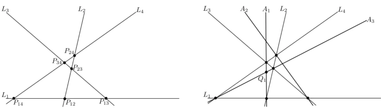
The construction of the model Γ-surfaces and the proof of Theorem 3.3.1 will be carried out for each family of graphs individually. This is done in Section 3.5. We outline our general approach below. Fix a graph Γ on the list of dual graphs. We construct a model Γ-surface ( ˜Z,E,˜ σ˜) as follows. We start with a curve C in the plane, and obtain the surface ˜Z by blowing up the plane repeatedly. The curve ˜E is obtained by taking the proper transform ofC together with some of the exceptional divisors of the blow-ups. The curve C and the points where we blow up must be chosen carefully so that the intersection pairing of ˜E is compatible with the graph Γ. We introduce some notation to describe this situation.
Definition 3.3.2. A Γ-surface (Z, E, σ) isconstructed by blow-ups if there is a birational morphism
π:Z→P2.
Such π factors into
π :Z =Zn−→πn Zn−1
πn−1
−−−→ · · · π2
−→Z1
π1
−→Z0 =P2,
where each πi is the blow-up of a point pi ∈ Zi−1. Denote by ei ⊂ Z the (proper transform of
the) exceptional divisor of πi. Let C =π(E), soE is the proper transform ˆC union some of the ei. Let E=S
Ej,C =S
Definition 3.3.3. We sayπ isgood if the points pi are uniquely determined by the plane curves Cj with their labels.
In other words, a blow-up construction is good if there are no choices involved other than the initial plane curveC. This is the case for example if theCj are all lines and eachpi is an intersection
point of two of them.
To prove the uniqueness (Theorem 3.3.1), let (Z, E, σ) be another Γ-surface with the same
I ⊂ D(Γ) as the model. We want to find rational (−1)-curves on Z that we can blow down in a manner that reverses the construction of ˜Z. Since we have knowledge of the associated I, the discussion in Section 3.1.1 implies that there are line bundles with the intersection properties we need. The bulk of the work is to show that these line bundles are in fact represented by irreducible rational (-1)-curves. After blowing down, the image of E is then a curve in the plane with the same intersection properties of the curveC of the construction. The uniqueness follows once we show C
is the unique plane curve with these properties.
The following lemma is the main technical tool used in the proof. It expresses the idea that if two Γ-surfaces correspond to the same I ⊂D(Γ), and we can find (−1)-curves in “the right places”, then we can blow down in a way that reverses the blow-up construction.
Lemma 3.3.4. Suppose π : Z → P2 is a good construction of (Z, E, σ) by blow-ups, and that (Z, E, σ) and (Z0, E0, σ0) correspond to the same self-isotropic I ⊂D(Γ). Let α: PicZ −→∼ PicZ0 be the isomorphism of Section 3.1.1. Ifα(ei)∈PicZ0 is represented by an irreducible curve e0i for each exceptional (-1)-curveei ⊂Z, then
(a) Z0 is constructed by blow-ups π0:Z0 →P2.
(b) There is an isomorphism φ: (Z, E, σ)−→∼ (Z0, E0, σ0) inducingα =φ∗ if and only if there is an automorphism ψ:P2 −→∼ P2 withψ(Cj) =Cj0 for all j.
Proof. (a) Blowing down e0n, . . . , e01 (in the reverse order as the blow-up construction) gives a birational morphism π:Z0 →S for some rational surfaceS. The invariant KZ0·KZ0 depends
only on Γ (see Remark 3.4.3, below) and is well-behaved under blowing up or down. So