Dynamics of continuously stratified and two-layer
incompressible Euler fluids and internal waves
Shengqian Chen
A dissertation submitted to the faculty of the University of North Carolina at Chapel Hill in partial fulfillment of the requirements for the degree of Doctor of Philosophy in the Department of Mathematics.
Chapel Hill 2013
Approved by:
David Adalsteinsson
Roberto Camassa
Jingfang Huang
Richard M. McLaughlin
Abstract
SHENGQIAN CHEN: Dynamics of continuously stratified and two-layer incompressible Euler fluids and internal waves.
(Under the direction of Roberto Camassa.)
The first part reveals a phenomenon in fluid mechanics that can be viewed as para-doxical: horizontal momentum conservation is violated in the dynamics of a stratified ideal fluid filling an infinite horizontal channel between rigid bottom and lid boundaries, starting from localized initial conditions, even though external forces only act on the vertical direction. The paradox is shown to be a consequence of the rigid lid constraint coupling through incompressibility with the infinite inertia of the far ends of the chan-nel, assumed to be at rest in hydrostatic equilibrium. By the perturbation theory based on small density variance, an analytical study quantifies the momentum development at the initial time. These results are compared with direct numerical simulations for variable density Euler fluids.
The second part is a numerical study of strongly nonlinear models for internal waves. We emulate numerically the generation of solitary wave motivated by a laboratory ex-periment. The dam-break problem for internal waves can be solved by direct numerical simulations (DNS). By smoothing out the dam and symmetric extension of the wave tank, the strongly nonlinear model is ready for implementation. The Kelvin-Helmholtz instability associated with the model is treated by a time-dependent low-pass filter. The regularized strongly nonlinear model with less-restrictive stability criterion is also considered. The snapshots of the models and DNS show excellent agreements between models and DNS. The effect of numerical filters are considered to behave as reducing dissipation.
Acknowledgments
First and foremost I want to thank my advisor, Dr. Roberto Camassa, for his en-couragement, patience, and rigorous yet pleasant training during these years, which have directly contributed to my general understanding of fluid mechanics and mathe-matical modeling. His childlike enthusiasm and curiosity of science have greatly influ-enced my way of thinking about and performing research. I feel really fortunate to have the opportunity to work under his supervision so that the process of solving problems is composed of joyful intellectual stimulations.
I also wanted to thank the members of my committee for all the suggestions they gave me in writing this thesis. I am greatly indebted to the entire applied math faculty. I want to thank Dr. Jingfang Huang for years of friendship and encouragement when I felt puzzled, confused about directions of my future career.
I am very grateful to Dr. Ann Almgren for her invaluable help with the numerical work and to Dr. Wooyoung Choi and Dr. Tae-Chang Joe for illuminating discussions. I want to thank Dr. Avadh Saxena, who kindly hosted me during a summer internship at LANL. During my stay at LANL, I had many useful discussions with Dr. J. Mac Hyman, for which I thank him. I also want to thank Dr. Gregorio Falqui, who invited me for a visit at University of Milano - Bicocca. And thanks to Dr. Giovanni Ortenzi and Dr. Marco Pedroni, with whom I initiated one of my thesis topics. For data anal-ysis, I have used extensively DataTank. I thank its creator, Dr. David Adalsteinsson for all his help.
sug-gestions. Also I want to thank my dear officemate, Claudia Falcon, for the positive energy she always brings to me. I am also indebted to so many friends who helped me accommodate in a foreign country.
Table of Contents
List of Figures . . . ix
List of Tables . . . xiv
1 General introduction . . . 1
2 Effects of inertia and stratification in incompressible ideal fluids: pressure imbalances by rigid confinement . . . 6
2.1 Introduction . . . 6
2.2 The physical system and its governing equations . . . 11
2.2.1 Pressure imbalances and horizontal momentum . . . 12
2.2.2 Smallρ∆ limit and the scaling relation between P∆ and ρ∆ . . . 16
2.2.3 Interfacial pressure imbalance and total vorticity . . . 19
2.3 Long-wave models . . . 21
2.3.1 Equations of motion . . . 23
2.3.2 Effects of dispersion . . . 24
2.4 Full Euler system: pressure jump att=0 in the smallρ∆ asymptotic limit 27 2.4.1 The small ρ∆ expansion . . . 27
2.4.2 Comparison with the long wave model . . . 33
2.4.3 Special initial conditions: piecewise-constant interfaces . . . 33
2.4.4 Special initial conditions: linear interfaces . . . 38
2.5 Dam-breaking class . . . 41
2.6 Time evolution: numerical results . . . 45
2.6.1 The effect of infinite inertia . . . 48
2.7 Time derivative of �p�∆ att=0 . . . 55
2.8 Conclusions . . . 57
3 An extended application for the strongly nonlinear internal wave models . . . 60
3.1 Introduction . . . 60
3.2 Motivations . . . 63
3.3 Mathematical models . . . 64
3.3.1 Governing equations . . . 64
3.3.2 Strongly nonlinear internal wave model . . . 65
3.3.3 Regularized nonlinear long wave model . . . 66
3.4 Numerical algorithms . . . 67
3.4.1 Direct numerical simulations for Euler equations . . . 67
3.4.2 Strongly nonlinear model . . . 68
3.4.3 Regularized model . . . 70
3.4.4 Artificial filter for long wave models . . . 71
3.5 Results . . . 72
3.5.1 Parameter set-up . . . 72
3.5.2 The effect of gate smoothing . . . 75
3.5.3 Small amplitude waves . . . 76
3.5.4 Moderate amplitude waves . . . 78
3.5.5 Large amplitude waves . . . 78
3.5.6 Choice of the optimal filter . . . 82
3.5.7 Primary wave forming solitary waves . . . 83
3.5.8 Horizontal shear velocity reconstruction . . . 85
3.6 Discussion . . . 88
4 Weakly nonlinear models for internal waves . . . 90
4.1 Introduction . . . 90
4.3 The strongly nonlinear model . . . 93
4.4 The Kortwerg-de Vries equation . . . 94
4.5 Weakly nonlinear models for bi-directional waves . . . 98
4.5.1 The two-layer Kaup model . . . 98
4.5.2 Regularized Kaup equations . . . 102
4.5.3 The two-layer Boussinesq equations . . . 106
4.5.4 The derivation of KdV equation from the Kaup equation . . . . 111
4.6 Higher-order uni-directional models . . . 115
4.6.1 Choice ofµ for conserved quantity . . . 116
4.7 The solitary waves produced by an arbitrary initial disturbance . . . 118
4.7.1 Solutions for the two-layer KdV equation . . . 120
4.7.2 Solutions for the two-layer weakly nonlinear models for bi-directional waves . . . 122
4.7.3 Higher order uni-directional model . . . 128
4.8 Discussion . . . 129
A Translational invariance and symmetries . . . 131
B Boundary effects in air water systems . . . 137
C Independent direct numerical simulations . . . 139
C.1 Solitary wave collisions . . . 139
C.2 Dam-break problem . . . 140
D Codes for models . . . 142
D.1 The strongly nonlinear model . . . 142
D.2 The regularized Kaup equations . . . 165
D.3 The Boussinesq equations . . . 173
D.4 The KdV equation . . . 185
D.5 Higher order uni-directional model . . . 195
List of Figures
2.1 A two-layer configuration with different asymptotic heights. . . 12 2.2 The contours for Stokes theorem in the case of a two-layer fluid. . . 20 2.3 Sketch of a typical interface configuration for a two-fluid density
distri-bution for which boundary contridistri-butions are relevant. . . 22 2.4 A two-bump configuration. Only whenS is comparable with the typical
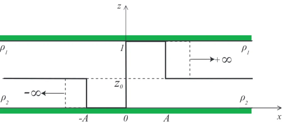
width of the bumps P∆ is nonzero. . . 26 2.5 Initial hook-like configuration for a two-fluid density distribution in an
x-infinite channel between two rigid plates located at z = 0,1. . . 35 2.6 (a) Full hook case, with A2 −A1 = A3 −A2 = 1.5, z3 = z0, z1 = 0,
z2 = 1, ρ∆ = 0.01 (crosses), ρ∆ = 0.1 (diamonds), from numerics ( § 2.6), theoretical value (solid line) from asymptotics ρ∆ → 0 . (b) Kink-like case, with A2 −A1 =A3 −A2 = 1.5,z1 = 0.3, z2 = 0.8, z3 = 0.5, ρ∆ = 0.01 (crosses), ρ∆ = 0.1 (diamonds), from numerics ( § 2.6), theoretical value (solid line) from asymptotics ρ∆ →0 (equation (2.71)). 36 2.7 Pressure imbalance P∆ vs. density difference ρ∆. Theory (solid line)
from equation (2.71) and VARDEN simulation (dots). The interface is a hook (figure 2.5) with parameters given by z0 = z3 = 0.5, z1 = 1,
z2 = 0, andA2−A1 =A3−A2 = 1.5 as in figure 2.6(a). The 2:1 slope is maintained up to density differences as large as ρ∆ �0.2 (in units of ρ2). 37
2.8 The special configuration of a staircase hook for a two-fluid density dis-tribution in an x-infinite channel between two rigid plates located at
z = 0,1. . . 38 2.9 The “incline hook” configuration for a two-fluid density distribution in
an x-infinite channel between two rigid plates located atz = 0,1. . . . 39 2.10 The piecewise constant vs. linear configurations for a two-fluid density
distribution in an x-infinite channel between two rigid plates located at
z = 0,1. . . 40 2.11 Dam-break configuration for a two-fluid density distribution. The
pres-sure is everywhere continuous (and so, ∂zp1 = ∂zp2 at the interface
x= 0) with the jump condition for its normal derivative at the interface
∂xp1 = (ρ1/ρ2)∂xp2. . . 42
2.13 Sketch of the fluid test domain and its symmetrical padding by wings of increasing length, doubling and quadrupling the period as shown. . . . 47 2.14 Density field from the numerical simulation of the evolution from the
initial data in the 1232 cm long tank with the center 308 cm test section marked by the vertical lines. . . 47 2.15 (a) Horizontal momentum time evolutions for the test section embedded
in progressively larger periodic domains, starting from the same initial condition. The solid line correspond to the rigid wall boundaries. (b) Time series of fluxes Q(t) with respect to increasing period L, for the same cases as (a). The flux decreases as 1/L in response to the larger inertia of the channel “padding” wings. . . 49 2.16 (a) Pressure jump and (b) total vorticity time history for the dam-break
initial condition sketched in figure 2.11, in the time interval 0s < t <2.8s
with 512 (solid line) and 256 (dotted line) vertical points resolutions. The initial velocities of the fluids are zero, the fluid densities are ρ1 =.9 and
ρ2 = 1 and the height of the channel is fixed to 1. . . 52 2.17 (a) Same as figure 2.16 but for the “hook with sliver” initial condition
(figure 2.5) with z0 =z3 = 0.5,z1 = 0.1 andz2 = 0.9. . . 53 2.18 (a) Same as figure 2.16 but for “complete hook” initial condition
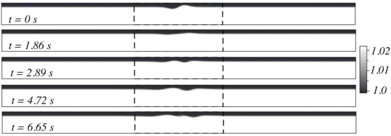
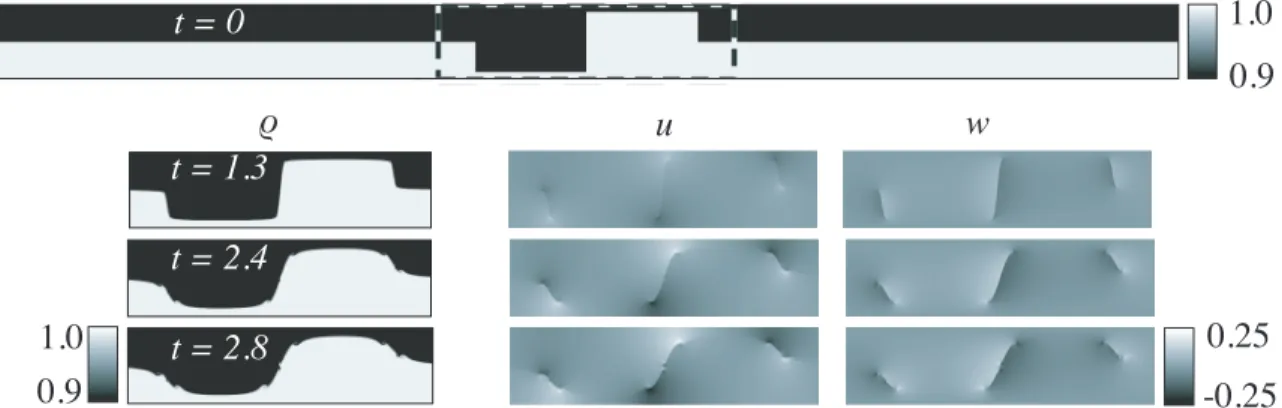
(fig-ure 2.5) with z0 =z3 = 0.5, z1 = 0 andz2 = 1. . . 53 2.19 Snapshots of density ρ and velocities (u, w) (for horizontal and
verti-cal component, respectively) for the time evolution of motion with the dam-breaking initial condition sketched in figure 2.11. Resolution is 512 vertical points, with physical parameters for this computation listed in the caption of figure 2.16. The initial density configuration is depicted in the top panel, which also illustrates the actual computational domain and its aspect ratio. . . 54 2.20 Same as figure 2.19 but for the “hook with sliver” initial condition case
(figure 2.5). Physical parameters listed in caption of figure 2.17. . . 54 2.21 Same as figure 2.19 but for the “complete-hook” initial condition case
2.22 Convergence of numerical algorithm for the “hook with sliver” initial data. Plotted here is the density difference at t = 2.8, generated by subtracting off the density from computations with 512 and 256 (ver-tical) nodes. Only the central portion (1/3 of the total length) of the channel is shown. For initial conditions that do not smooth the density jump, the resolution error becomes noticeable along the interface, where slight differences in its position in addition to numerical diffusion lead to nonzero density differences between the two computations. . . 55 3.1 Dam-break experiment setup . . . 72 3.2 Initial condition for long wave models by a symmetric extension of the
wave tank and smoothed gate. . . 73 3.3 Snapshots of VarDen simulations. Top: H10LD1; bottom: H50LD1 . . 74 3.4 Snapshots at T = 80 s from VarDen simulations with different λ,
corre-sponding to different smoothing effect for runs H10’s (a) and H50’s (b). Solid black: λ = 0.1 cm−1; solid gray: λ = 0.2 cm−1; dash-dot black: λ =∞ (no smoothing). . . 75 3.5 Snapshot of H10LD1 atT = 80 s. Solid: mean density isopynocline from
VarDen simulation; dashed: strongly nonlinear model; dotted: regular-ized model. The three vertical lines are at locations x= 1420, 1510 and 1610 cm . . . 77 3.6 Time series of relative energy loss from VarDen simulations (a1, a2, and
a3), the strongly nonlinear model (b1, b2, b3), and the regularized model (c1, c2, c3), with number 1, 2 and 3 denoting runs H10LD1, H20LD1 and H50LD1, respectively. . . 79 3.7 Snapshot of H20LD1 at T = 80 s. Solid: isopynocline of the mean
den-sity from VarDen simulation; dashed: strongly nonlinear model; dotted: regularized model. The three vertical lines are at locations x = 1525, 1610 and 1700 cm. . . 80 3.8 Snapshot of H50LD1 at T = 80 s. Solid: isopynocline of the mean
den-sity from VarDen simulation; dashed: strongly nonlinear model; dotted: regularized model. The three vertical lines are at locations x= 1550 cm, 1610 cm and 1800 cm . . . 80 3.9 Convergence study for run H50LD1 in VarDen simulations with different
3.10 Solutions from the strongly nonlinear model for run H50LD1 with fixed
C = 1.3 and different Kupp at T = 80 s. Solid: mean density isopycn-ocline from VarDen simulation; dashed black: Kupp = 0; dashed blue:
Kupp = 500; dashed red: Kupp = 900. . . 82
3.11 Time series of relative energy loss for the strongly nonlinear model with fixed C = 1.3 and different Kupp. Solid black: Kupp = 0; solid blue:
Kupp = 500; solid red: Kupp = 900; dashed purple: Kupp = 100; dashed
green: Kupp = 300; dashed orange: Kupp = 700. . . 83 3.12 The front half of the primary waves from models at timeT = 60 s (black
short-dashed), T = 80 s (black long-dashed) andT = 100 s (black solid), VarDen simulations at T = 100 s (red solid) traveling wave solutions from the strongly nonlinear model with matching amplitude atT = 100 s (green solid). (a1), (a2) and (a3) are from the strongly nonlinear model for runs H10LD1, H20LD1 and H50LD1; (b1), (b2) and (b3) are from the regularized model for the same runs. . . 84 3.13 Amplitudes (left) and phase locations (right) of the wave peak for H10LD1
(a), H20LD1 (b) and H50LD1 (c). Square: the strongly nonlinear model; cross: VarDen simulation . . . 86 3.14 Horizontal shear velocities reconstructions for runs H10LD1 (a), H20LD1
(b) and H50LD1 (c) at locations noted in figures 3.5, 3.7 and 3.8. . . . 87 4.1 The solitary wave solution from the Kaup equations with the physical
pa-rameters ρ1 = 0, ρ2 = 1 g·cm−3, h1 = 1.95 cm, h2 = 2 cm, g = 1 cm·s−2
corresponding ti the critical wavenumber kcritical = 0.86. The Fourier modes below this instability threshold are not sufficient for recovering the solution. Solid: solitary wave solution; dashed: solitary wave solu-tion with truncated Fourier coefficients satisfying the stability criterion. 102 4.2 Sketch off(U) in equation (4.82) with all possibilities for different values
of d1. Note that the gray curves do not lead to solitary wave solutions. 112 4.3 The relationship between traveling wave speed and amplitude with
pa-rameters in the laboratory experiments introduced in Chapter 3. Solid: strongly nonlinear; long dashed: Boussinesq; dotted: regularized Kaup; short dashed: Kaup model . . . 113 4.4 Traveling wave solutions from the strongly nonlinear model (solid green),
4.5 Traveling wave solutions from the strongly nonlinear model (solid), the higher-order unidirectional model with µ = ˜µ (dashed) and the KdV equation (dotted) matching amplitude awith physical parameters intro-duced in § 4.7. (a): a = −1 cm, (b): a = −5 cm and (c): a = −10 cm. . . 119 4.6 Snapshot of time evolution at T = 500 s from the KdV equation. . . 119 4.7 Snapshot of the time evolution from the regularized Kaup equations
(dashed), the Boussinesq equations (dotted), the strongly nonlinear model (solid green) and the Euler simulation (solid) with the initial condition
hgate = 10 cm andLgate = 100 cm, at T = 500 s. . . 124 4.8 Snapshot of the time evolution from the regularized Kaup equations
(dashed), the Boussinesq equations (dotted), the strongly nonlinear model (solid green) and the Euler simulation (solid) with the initial condition
hgate = 10 cm andLgate = 200 cm, at T = 500 s. . . 125 4.9 Snapshot of the time evolution from the regularized Kaup equations
(dashed), the Boussinesq equations (dotted), the strongly nonlinear model (solid green) and the Euler simulation (solid) with the initial condition
hgate = 1 cm andLgate = 100 cm, at T = 500 s. . . 126
4.10 Initial conditions of ζ with the set-up from the dam-break experiment (solid) and a long wave in the expression of equation (4.119) with the same amplitude (hgate = 1 cm) (dotted dash) . . . 127 4.11 Snapshot of the time evolution from the regularized Kaup equations
(dashed), the Boussinesq equations (dotted), the strongly nonlinear model (solid green) and the Euler simulation (solid) with the initial condition
hgate = 1 cm, atT = 500 s. . . 128 4.12 Snapshots for higher-order uni-directional model with µ = ˜µ at T =
80 s with domain L = 2464 cm. Thick gray: Euler; solid: the strongly nonlinear model; dashed: higher-order uni-directional model withµ= ˜µ; dotted: the KdV equation . . . 129 C.1 Snapshots of collisions of two solitary waves generated from dam-break
at two ends. (a): symmetric case; (b) asymmetric case with different gate height at two ends . . . 140 C.2 Time series ofP∆ for solitary wave collisions with symmetric dam set-up
(dashed) and asymmetric dam set-up (solid) . . . 141 C.3 Snapshots of the dam-break problem with a gate in the dimension of
List of Tables
2.1 Comparison of pressure imbalances P∆/ρ
2
∆ as predicted by long-wave model and full Euler results for interface (2.47) with asymptotic height
z0 = 1/2. . . 32
3.1 Labels for numerical runs with different parameters . . . 74 3.2 Numerical values for amplitudesaand phasesXof the primary wave from
VarDen simulation, the strongly nonlinear model and the regularized model for runs H10LD1, H20LD1 and H50LD1 at T = 80 s. . . 80
4.1 Tracking front wave amplitude aKdV and phase XKdV from two-layer
KdV model for the two-layer dam-break problem with Lgate = 100 cm and hgate = 10 cm at different snapshots. . . 122 4.2 Tracking front wave amplitudes a and phases X from the two-layer
reg-ularized Kaup equations and the Boussinesq equations for the two-layer dam-break problem with Lgate = 100 cm and hgate = 10 cm at different snapshots. . . 124 4.3 Values of amplitudes from inverse scattering predictions from Kaup
equa-tions and time evoluequa-tions from regularized Kaup equaequa-tions, the Boussi-nesq equations and the Euler simulations atT = 500 s forLgate = 200 cm and hgate = 10 cm. . . 126 4.4 Amplitudes and phases of front waves from models and the Euler
Chapter 1
GENERAL INTRODUCTION
Ideal fluids are theoretical simplifications of real fluids obtained by ignoring viscosity and thermal conductivity. Such idealization is useful in many cases, such as flows considered in oceanography, where the Reynolds numbers are high. The mathematical description for ideal fluids are the Euler equations, representing conservation of mass, momentum and energy, which can be viewed as the Navier-Stokes equations in the limit of zero viscosity and heat conductivity. This thesis is concerned with incompressible ideal fluids with variable densities. Such setup allows for internal waves, which in their simplest occurrence can be seen as propagating at the interface between two fluids of different densities. Such ultimate simplification may in fact still be useful in oceanographic settings, and can be closely approximated in laboratory conditions.
show that they are usually long with respect to the average fluid depth, e.g., wavelengths be of the order of 10 kilometers with the layer depths less than 1000 meters (Apelet al. [2], Helfrich & Melville [24]). Hence, in order to gain insight into wave dynamics of the Euler equations, whose solution for the most part are amenable to numerical methods only, it is useful to study asymptotic models built on the long wave assumption. These models can be derived with further simplifying assumptions such as idealized domains horizontal directions extending to infinity or confined in periodic lattices.
This thesis studies three problems concerning the derivation and properties of long internal-wave models from incompressible ideal fluids with variable densities. Each of these problems is essentially self contained:
1. The mathematical idealization of extending the container of the fluid to infinite lengths simplifies the physical problem. On the other hand, this setup seemingly brings in some paradoxical property, which are analyzed the first part of this work in some detail.
2. The model asymptotic derivation assumes initial conditions that satisfy the long wave assumption. When this is violated, how robust are the models with respect to the long time evolution with respect to the parent Euler system? This question is taken up for a class of initial and boundary conditions of relevance in laboratory experiments in the second part of this thesis.
3. The previous study shows that solitary waves are a dominant feature of the dy-namics of a certain class of initial data. Can the presence and features of these waves be analytically predicted from models? This is the subject of the third part of this work.
pycnocline displacements, i.e., the scales associated with internal wave motion greatly exceed the scales of the surface (barotropic) waves (Vlasenkoet al. [36]).
of strongly nonlinear internal waves in two-fluid systems.
Appendix A reviews the Lagrangian and Hamiltonian formalism of the Euler equa-tions, in particular adapting it to the two-fluid configuration, which allows the frame-work of conservation laws to be established from a more general standpoint.
Appendix B briefly examines the limiting case of “air-water” systems, in which one of the densities goes to zero. Non-trivial boundary effects on the pressure imbalance which are masked by the opposite near-density limit emerge in this case, due to the interface profile touching the channel plates along some intervals.
In Chapter 3, we conduct numerical experiments with direct Euler simulations and two long internal wave models for large amplitude waves: the strongly nonlinear model (Choi & Camassa [15]) and the regularized model (Choi et al. [14]). Studies of these models have mostly been limited to traveling wave solutions only. Our numerical exper-iments are motivated by laboratory experexper-iments (Grue et al. [23]), with stratification achieved by pouring a layer of fresh water above a layer of brine in a long rectangular tank. By adding a volume of fresh water behind a gate which is lowered at one end of tank, a corresponding mass of the brine then slowly moves to the other side of the gate such that hydrostatic balance is maintained. By removing the gate, the initial pycno-cline depression develops into a leading solitary wave propagating ahead of a transient dispersive wave train. The mathematical formulation of this dam-break internal wave problem is that of a step function representing the initial interface displacement, which clearly does not satisfy the long wave assumption for initial data of the models. In fact, it turns out that the models are sufficient to numerically predict front waves with low computational cost and remarkable accuracy when comparing to the full Euler simulations.
Chapter 2
EFFECTS OF INERTIA AND STRATIFICATION IN
INCOMPRESSIBLE IDEAL FLUIDS: PRESSURE IMBALANCES BY RIGID CONFINEMENT
This Chapter is collaborative work with Gregorio Falqui, Giovanni Ortenzi and
Marco Pedroni. The content of this Chapter is from our published articles [8] and
[9] in Journal of Fluid Mechanics.
2.1 Introduction
Among the many areas of classical mechanics, fluid dynamics arguably holds a special distinction for being a rich source of the sort of paradoxes that often arise from simplifying limit assumptions. Thus, for instance, the limit of zero viscosity gives rise to D’Alembert’s paradox on the drag experienced by rigid bodies moving in ideal fluids, while the opposite limit of dominating viscous stresses leads to the Stokes or Whitehead paradoxes of unphysical divergences for the same problem.
lead to horizontal forces by action-reaction mechanisms due to the constrained motion, and so horizontal momentum conservation cannot in general be expected to hold for a stratified Euler fluid filling a finite domain enclosed by a rigid boundary. However, we shall see below that for a domain extending horizontally to infinity the infinite inertia possessed by the far fluid at rest acts as an effective lateral boundary, giving rise to violation of horizontal momentum conservation. While stratification is necessary for creating the relative inertia of the lateral fluid at rest, a subtlety of this effect is that incompressibility is also required to transmit forces arising from finite-range motion instantaneously all the way to infinity. Accordingly, the “light-cone” provided by the maximum speed of propagation of internal baroclinic modes gives a rough estimate of the boundary of the exterior region that can be considered as contributing to an effective-wall lateral confinement.
This violation can be viewed as surprising, as the only acting body-force field is the vertical gravity and the fluid is free to move laterally. Possibly the first mention of this peculiar feature of stratified fluid dynamics can be traced back to Benjamin [5], in his investigation of the Hamiltonian formalism for inviscid incompressible fluids. Despite the relatively long time elapsed, it appears that Benjamin’s observation about (in his own words) “this curious fact” have been largely ignored since.
in the limit of a homogeneous fluid). Small density variations are common to many applications such as geophysics, however the large scales often involved in such appli-cations justify considering the idealized set-up of laterally infinite fluids and might lead to non-negligible cumulative effects, even when these are small over local scales. Of course, the implications arising from considering rigid lids upper constraints in these applications remain to be seen; however, this limiting case may be relevant for estab-lishing a comprehensive framework in which the dynamics of the incompressible limit for density-stratified fluids can be properly interpreted.
We shall mainly deal with incompressible, inviscid two-layer (Euler) fluids of con-stant different densities ρ2 > ρ1, separated by an interface located at z =η(x, t) (not necessarily smooth), where (x, z) are horizontal and vertical Cartesian coordinates in the plane. This choice is convenient for analytical purposes, and while numerically chal-lenging, it can nonetheless be implemented in direct simulations of stratified Euler flows. While restrictive, the two-layer assumption can be representative of the dynamics of Eu-ler fluids with smooth density variations as well (see, e.g., Camassaet al.[10], Camassa & Tiron [12]). In particular, for two-layer fluids in which the interface height is the same at±∞, the pressure imbalanceP∆ ≡limx→+∞p(x, η(x, t))−limx→−∞p(x, η(x, t)) is equal to the difference of the pressures p(±∞, z0) for any reference height z0, as it could be obtained from Benjamin [4] for smooth stratifications.
Our main focus will be on initial conditions with null velocity and small ρ∆ ≡ ρ2−ρ1. This choice, as shown below, restricts the effects on the pressure imbalance of stratification at initial times to orderρ2
particular, the setting of zero-velocity configurations will be instrumental in Section 2.4, where we shall adopt a perturbative point of view (in the limit ρ∆ → 0) to solve the elliptic equations which determine the pressure att= 0. Some compact expressions for the pressure imbalances can then be obtained. Our analysis will be carried out directly on the Euler equations of motion in two dimensions; however, as a kind of benchmark for testing ideas, we shall also consider long-wave one-dimensional reductions of our two-dimensional set-up, such as the strongly nonlinear model introduced in Choi & Camassa [15] for the description of strongly nonlinear internal waves in two-fluid systems. We will also briefly review the Lagrangian and Hamiltonian formalism of the Euler equations, in particular adapting it to the two-fluid configuration, which allows the framework of conservation laws to be established from a more general standpoint.
More specifically, the layout of this chapter is as follows. In § 2.2 we introduce the set-up of our physical system within the Euler formalism, and, in particular, focus on the relation between non-conservation of horizontal momentum and the pressure imbalanceP∆. §2.2.2 describes the asymptotic behavior ofP∆ with respect to the small
Next, in § 2.4 we discuss pressure imbalances with zero-velocity initial data for two-layer fluids. The exact problem of solving the Laplace equation for the initial pressure can be viewed as a form of Neumann-to-Dirichlet problem for a (two-layer) strip. We adopt a simple perturbative approach in the limit of small density difference
ρ∆, turning this problem into an iterative family of Poisson equations which allow for a closed-form integral expression for the second order termP(2)
∆ of the pressure imbalance associated with any interface profile z = η(x). In some cases (e.g., piecewise linear profiles) this expression easily yields explicit formulae forP(2)
∆ (which in suitable limits are expressed by Bernoulli-like polynomials). A sample of these formulae and their interpretation is contained in § 2.4.3 and § 2.4.4. In particular, within a certain class of initial data, we determine the configuration that maximizes the pressure imbalance. In § 2.5 the dam-break configuration is studied. At t = 0 an exact explicit value for �p�∆ can be obtained. The comparison of the theoretical results with full-Euler numerical experiments, in § 2.6, further illustrates the (short-time) dynamics arising from these pressure imbalances of these configurations and its effects on the horizontal momentum. Computations are performed with the VARDEN algorithm (Almgrenet al. [1]) which solves the inhomogeneous Euler equations. The two-layer (sharp interface) set-up can be viewed as a severe test for the code, which gets validated by the overall good agreement with the analytical results. In § 2.8 we discuss our findings and point to future work.
2.2 The physical system and its governing equations
We study the Euler equations for an ideal incompressible and inhomogeneous fluid subject to gravity,
vt+v· ∇v=−∇
p
ρ −gk, ∇ ·v= 0, ρt+v· ∇ρ= 0. (2.1)
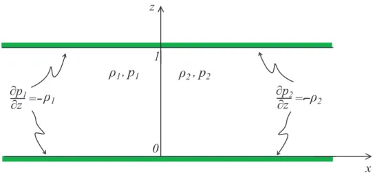
Here v = (u, v, w) is the velocity field with respect to Cartesian coordinates (x, y, z) oriented by unit vectors (i,j,k), with k directed vertically upwards, ρ and p are the density and pressure fields, respectively, and g is the constant gravity acceleration; all physical variables depend on spatial coordinates and time t. Besides their well known theoretical interest, this set of equations can be viewed as governing the motion of real fluids with sufficient accuracy whenever viscosity, compressibility and diffusivity effects can be considered small during the time evolution. In particular, the fluid domains we shall consider here are slabs in the (x, z) plane rigidly confined by horizontal plates of infinite extent located at z = zbottom ≡ 0 and z = ztop ≡ h. Our study will mainly
focus on two dimensionaly-independent dynamics, though it can be generalized to fully three dimensional cases. The Euler equations (2.1) are supplemented by the boundary conditions:
v(x,·)→0 for |x| → ∞, w(x,0) =w(x, h) = 0, (2.2)
with the fluid at the far ends of the channel in hydrostatic equilibrium,
∂p
ρ1 ρ2
w=0
w=0 z
-z+
u=0 u=0
Figure 2.1: A two-layer configuration with different asymptotic heights.
2.2.1 Pressure imbalances and horizontal momentum
Consider the Euler equations for the horizontal component of the fluid’s momentum
(ρu)t =−u(ρu)x−w(ρu)z−px. (2.4)
Assuming a smooth stratification and integrating this equation on the strip S = R× [0, h] yields the time variation of the horizontal component Π1 of the total momentum
d dtΠ1 =
�
S
(ρu)tdA=−
�
S
�
(ρu2)x+ (ρuw)z −ρu(ux+wz) +px
� dA
=− � h
0
��
R(ρu
2+p)
xdx
�
dz =−h(�p(+∞)� − �p(−∞)�),
(2.5)
where we used incompressibility and the asymptotic hydrostatic conditions (see also Benjamin [5]). Hereafter the symbol�f�stands for the (total) vertical channel average,
�f(·)� ≡ 1
h
� h
0
f(·, z) dz.
The two-layer case
the pressurepj, for each of the layers; in two dimensional Cartesian coordinates (x, z):
uj x+wj z = 0 (2.6)
uj t+ujuj x+wjuj z = −pj x/ρj (2.7)
wj t+ujwj x+wjwj z = −pj z/ρj−g. (2.8)
For a two-layer fluid, j = 1 (j = 2) will stand for the upper (lower) fluid, respectively, and ρ1 ≤ ρ2 must be assumed for stable stratification (see figure 2.1 for a sketch of this set-up). The boundary conditions at the interfacez =η(x, t) are the continuity of normal velocity and pressure
ηt+u1ηx =w1, ηt+u2ηx =w2, p1 =p2 ≡P at z =η(x, t), (2.9)
where P(x, t) denotes the interfacial pressure. Let us rewrite the Euler system (2.8) in terms of layer-averages (see, e.g., Wu [38] and Camassa & Levermore [11]). (For a smoothly stratified fluid, this is equivalent to singling out an intermediate level set of constant density z = η(x, t) and carrying similar manipulations since such a set will always be a material surface.) Layer-mean quantities ¯f are defined by
¯
fj(x, t)≡
1
ηj
�
[ηj]
f(x, z, t) dz , (2.10)
where ηj are the layer-thicknesses (i.e., η1 = h −η and η2 = η) and the intervals
of integration [ηj] are z ∈ (η, h) for the upper- and z ∈ (0, η) for the lower-layer,
(lower) fluid
ηj t+�ηjuj
�
x = 0 (2.11)
ρj(ηjuj)t+ρj
�
ηjujuj
�
x =−(ηjpj)x+ (−1) jη
xP , j = 1,2. (2.12)
Layer averages are just a local version of the integral form of the horizontal momentum balance for each layer, which can be expressed for a section of the channel by integrat-ing equations (2.12) over some x-interval L− ≤ x ≤ L+. The horizontal momentum balances of the upper (j = 1) and lower (j = 2) layer for this section are, respectively,
d�
1j
dt ≡
d dt
� L+
L−
ρjηjujdx+ρjηjujuj|LL+− =−ηjpj|LL+− + (−1)j
� L+
L−
ηxP dx , (2.13)
since neither the pressure at the rigid horizontal surfaces nor the external gravity field contribute horizontal components of forces. Taking into account that
2
�
j=1
ηjpj|LL+− =h(�p(L+)� − �p(L−)�),
and that the total horizontal momentum of the two-fluid’s system is the sum of the contributions of the individual layers, in the limit L± → ±∞ (e.g., L± = ±L) and Π�
1 →Π1, system (2.13) yields the two-layer analogue of Equation (2.5), i.e.,
dΠ1
dt =
dΠ11
dt +
dΠ12
dt =−h�p�∆, (2.14)
where�p�∆ ≡ �p(+∞)�−�p(−∞)�. In hydrostatic equilibrium the layer-mean pressures are
pj = (−1)jgρj
ηj
Taking this into account at±∞, we get
dΠ1
dt =
dΠ11
dt +
dΠ12
dt =−hP∆− 1 2ρ∆g(z
2
+−z−2)−ρ1gh(z+−z−), (2.16)
whereP∆ ≡limx→+∞p(x, η(x, t))−limx→−∞p(x, η(x, t)),
z−≡ lim
x→−∞η(x, t), z+ ≡x→lim+∞η(x, t), for all t, (2.17)
and ρ∆ =ρ2−ρ1. In particular, by comparing (2.14) and (2.16), we have
�p�∆ =P∆ +
ρ∆g
2h (z 2
+−z−2) +ρ1g(z+−z−),
so that if the asymptotic interfacial heights are the same at both far ends of the channel, equality between asymptotic imbalances of the interfacial pressure and of the mean pressure follows,
�p�∆ =P∆. (2.18)
It is interesting to view the pressure imbalance from the perspective of a center of mass for the stratified fluid. For a laterally unbounded channel, the total mass of the fluid is clearly infinite, and care should be taken to avoid divergent integrals. The local center of mass horizontal coordinate for a section of the channel between x=L− and x=L+
can be defined as
Xc�(t)≡ 1
M�
� L+
L−
x�ρ1η1(x, t) +ρ2η2(x, t)�dx , (2.19)
where
M� ≡
� L+
L− �
is the total mass of the fluid in the section. Differentiating with respect to time, and taking into account (2.11), yields
M� dX
� c
dt =
� L+
L−
(ρ1η1u1+ρ2η2u2) dx+
�
(Xc�−x)(ρ1η1u1+ρ2η2u2)����
L+
L− . (2.21)
For velocities that decay sufficiently fast at infinity the end-point terms in this expres-sion vanish and the right-hand-side is well defined in the limit L±→ ±∞, being equal to the total horizontal momentum Π1 of the fluid. Thus, the position of the center of
mass for a sufficiently long section of the channel moves in the direction defined by the total horizontal momentum, as can be expected.
2.2.2 Small ρ∆ limit and the scaling relation between P∆ and ρ∆
Some of the results of the previous subsection can be used to unravel a particular scaling of the momentum evolution with respect to stratification. In particular, we shall focus on the class of zero-velocity initial data. As we will see later, these initial conditions also allow to derive closed-form expressions for the initial pressure imbalance. From the equations of motion and, in particular, from the constraint η1 +η2 = h
we have
∂x
�
η1u1u1+η2u2u2+
1
ρ1η1p1+
1
ρ2η2p2
� =� 1
ρ2 −
1
ρ1
�
ηxP . (2.22)
If hydrostatic equilibrium at infinity is enforced, the layer-mean pressures are given by (2.15), so that in the case of equal asymptotic heights, that is, z− = z+ = z0, the interfacial pressure difference P∆ between the ends of the channel is
P∆(ρ∆) = P|
+∞
−∞ =
ρ∆
h1ρ2 +h2ρ1
� +∞
−∞
ηxP dx≡
ρ∆
h1ρ2+h2ρ1IP(ρ∆), (2.23)
the nonconservation of total momentum and vorticity, cannot arise in uniform density fluids. Next, and perhaps more remarkably, these phenomena cannot be detected in the Boussinesq approximation of neglecting density stratification in the inertial terms. Relation (2.23) further shows that P∆ scales at least linearly with ρ∆. Of course, the integral termIP also depends onρ∆, so that it cannot be concluded that this linear scaling has general validity. In fact, in the limit ρ∆ →0 with ρ2 fixed, the scaling can be different than linear. Assume that the interfacial pressureP admits the expansion
P∆(0) +P∆
�(0)ρ
∆ + 1 2P∆
��(0)ρ2
∆ +. . .
= 1
h1ρ2 +h2ρ1IP(0)ρ∆ +
1
h1ρ2+h2ρ1I
�
P(0)ρ∆2 +. . .
= 1
hρ1IP(0)ρ∆+ �
1
hρ1I
� P(0)−
h1 h2ρ2
1 IP(0)
�
ρ∆2+o(ρ∆2),
(2.24)
where o(ρ2
∆) denotes, as usual, terms going to zero faster than ρ
2
∆. This implies that
IP(ρ∆) → 0 as ρ∆ → 0 for localized displacements of the interface. Equating term by term yieldsP∆(0) = 0, as already manifest from (2.23). Now, for a homogeneous fluid, equation (2.16) shows that horizontal momentum is conserved if P∆(0) = 0. On the other hand, recalling that the time variation of each layer’s total horizontal momentum is
dΠ1j
dt ≡
d dt
� +∞
−∞
ρjηjujdx+ ρjηjujuj|+−∞∞=−ηjpj|+−∞∞+ (−1)jIP, j = 1,2, (2.25)
we can see that if the upper and lower layer momentum are separately conserved, then not onlyP∆ = 0, but also IP = 0. Indeed, the lateral equilibrium boundary conditions imply that for each infinite upper and lower layer the horizontal momenta are conserved if and only if
at all times, that is, if and only if
IP = 0 and P∆ = 0. (2.27)
Now, given thatρ∆ = 0 implies horizontal momentum conservation, and for zero initial velocities the initial value of each layer’s total horizontal momentum is clearly zero, the conserved value of the horizontal momentum in each layer is null for all times (and hence so is the total fluid’s horizontal momentum). Therefore (2.27) shows that the linear term in expansion (2.24) vanishes. Thus, for zero velocities, P∆(ρ∆) is at least quadratic in ρ∆, since from (2.24) we obtain
P∆ =
1
h1ρ2+h2ρ1I
�
P(0)ρ∆2+o(ρ
2
∆). (2.28)
Notice that this result is general for zero-velocity initial conditions. If the velocity of the system is different from zero, the difference of pressure between the ends of the channel can be expected, in general, to scale linearly with the density difference ρ∆, at least initially in time.
We remark that, if different asymptotic heights are enforced on the fluid’s configu-ration, formula (2.23) has to be modified as
ρ∆
ρ1ρ2IP(ρ∆) = �
h−z+
ρ1 +
z+ ρ2
�
P(+∞)− �
h−z−
ρ1 +
z− ρ2
�
P(−∞) +gh(z+−z−).
2.2.3 Interfacial pressure imbalance and total vorticity
Next, we briefly examine how the asymptotic interface pressure differentialP∆ is re-lated with variation of the total vorticity. This link can be obtained from the Helmoltz-type equation for the vorticity,
ωt+∇ ×(ω×v) =−∇
� 1
ρ
�
× ∇p. (2.30)
For a system in the strip S =R×[0, h], the total vorticity is
Γ= �
R×[0,h]
ωdA . (2.31)
Its time variation follows directly by integrating (2.30), and by using the Green-Stokes’ formula. Taking into account the boundary conditions on the velocity field yields
dΓ
dt =
�
R×[0,h]∇ p× ∇
� 1
ρ
�
dA . (2.32)
Notice that any barotropic component of the pressurepb =pb(ρ) will not contribute to
this formula, which ultimately rephrases the content of the Bjerknes theorem (see, e.g., Yih [40]) applied to the whole fluid domain.
We now consider the two-layer case. In this case, ρ = ρ2 −H(z −η(x, t))ρ∆ (by denoting the Heaviside function asH), and hence the gradient of 1/ρ is
∇ �
1
ρ
� =
−ηx
1 ρ∆
ρ1ρ2δ(z−η(x, t)), (2.33)
= +
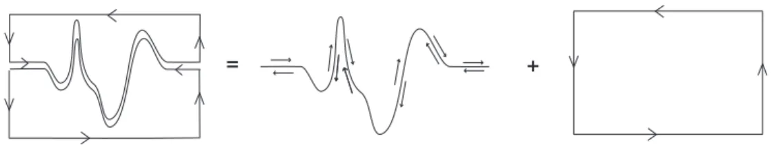
Figure 2.2: The contours for Stokes theorem in the case of a two-layer fluid.
continuous. In our case, while the component of the pressure gradient normal to the interface suffers a jump, the tangential component is continuous, and hence so is the
δ multiplier. We have
∇p× ∇ �
1
ρ
�
=−(px+pzηx)
ρ∆
ρ1ρ2δ(z−η(x, t))j, (2.34)
wherejis the unit vector normal to the fluid plane. Similar care is needed to apply the Green-Stokes formula in the two-layer case, because the integrand is again singular at the interface, in general. The contour of integration has to be modified by separating the different domains where the density is constant, thereby breaking the contour path used in the smooth density case into two paths enclosing the domain of each fluid. This decomposition, depicted in figure 2.2, reduces the problem to evaluating the contour integration at the interface, because the contributions of the channel boundaries vanish for the same reason as for the smooth density case. In this chapter we will be concerned mainly with the case of zero-velocity initial conditions, so that the fluid vorticity ω is concentrated on the interface γ in a vortex sheet (see also Yih [40], p. 14). Therefore the kinetic contribution to dΓ/dt is
�
γ
(ω×v1)·dr− �
γ
(ω×v2)·dr= �
γ
ω×(v2−v1)·dr. (2.35)
using (2.34) we can express the time variation of the total vorticity in terms of the (interface) pressure imbalance as
dΓ dt = � ∞ −∞ �� h 0
(px+pzηx)
ρ∆
ρ1ρ2δ(z−η(x, t)) dz
� dx
= ρ∆
ρ1ρ2
� ∞
−∞
(px+pzηx)|z=η(x,t)dx= ρ∆
ρ1ρ2
� ∞
−∞
dP dx dx
= ρ∆
ρ1ρ2
�
P(+∞)−P(−∞)� = ρ∆P∆
ρ1ρ2 ,
(2.36)
where we have used the definitionP(x) =p(x, η(x)).
Formula (2.36), connecting the time variation of the total vorticity with the asymp-totic pressure imbalance, has to be corrected if the interface touches the boundary of the channel. Indeed, let C be the set in which the interface coincides with one of the boundaries (see figure 2.3). Forx∈ C and everyz ∈[0, h] the gradient of the density is zero, so that the set C ×[0, h] does not contribute to the total vorticity time-variation. Therefore dΓ dt = ρ∆ ρ1ρ2 �
R/C
dP dx dx=
ρ∆ ρ1ρ2
�
P∆−
n
�
i=1
�
p�xRi , η
�
xRi
��
−p�xLi, η
�
xLi
��� �
. (2.37)
We remark that the correction terms might be, in some cases, dominant. Indeed, for vanishing velocity initial configurations,P∆ behaves asρ
2
∆, while the point contributions can produce linear terms in ρ∆.
2.3 Long-wave models
xnL xnR
x2L x
2 R
x1L x1R ρ1
ρ
2
z0
Figure 2.3: Sketch of a typical interface configuration for a two-fluid density distribution for which boundary contributions are relevant.
2.3.1 Equations of motion
For a two-layer incompressible Euler fluid in a channel of height h, the equations of motion (2.11)–(2.12) can be written as
uit+uiuix+ (−1)igηix =−
Px
ρi
+Di(ui, vi, ηi), ηit+ (ηiui)x = 0, i= 1,2, (2.38)
whereη1+η2 =h, and the terms denoted byDilump all the contributions from pressure,
vertical velocity components and from switching layer-averages with products. Shallow water long-wave models can be derived from this in the case when the layer thicknesses are small with respect to a typical wavelenght L, by retaining only the leading order terms in Di, and provide effective approximations of (two-layer) incompressible Euler
fluid (see. e.g., Choi & Camassa [15]). Denoting the small parameter of the model by
δ≡h/L, at the first order inδ the hydrostatic equilibrium is valid everywhere and the relations (2.15) hold not only asymptotically but along the whole channel. Also, at this order Di = 0, i.e., system (2.38) is turned into its dispersionless limit
uit+uiuix+ (−1)igηix =−
Px
ρi
, ηit+ (ηiui)x = 0, i= 1,2. (2.39)
In case of zero asymptotic velocities the total fluxQ(t)≡η1u1+η2u2 is zero. Solving for Px the dispersionless equations (2.39) and using the constraint η1 +η2 =h, yields
for the interface pressure asymptotic difference the (dispersionless) formula
P∆ =h � ∞
−∞
(u1 u2)x
η1/ρ1+η2/ρ2dx. (2.40)
rela-tive inertia of the stratified fluid, and not to the relarela-tive buoyancy. Still, formula (2.40) shows thatP∆ = 0 when the interface is flat (with any averaged velocities). On general grounds, this can also be seen from (2.23), since ηx = 0 for a flat interface. However,
the dispersionless formula (2.40) predicts P∆ = 0 for zero velocities as well, which is not true in general. Next, we show how such a pressure imbalance can be qualitatively understood by restoring the dispersive terms in the strongly nonlinear model.
2.3.2 Effects of dispersion
The fact that for zero-velocities formula (2.40) fails to yield a nonzero value for
P∆ suggests that for small velocities (or interface profile) the dispersive terms Di of
Equation (2.38) could play a significant corrective role. In fact, if such terms are nonzero, then relation (2.40) turns into
P∆ = � +∞
−∞
�
η1 ρ1 +
η2 ρ2
�−1
[h(u1u2)x+ (η1D1+η2D2)] dx . (2.41)
The first nontrivial dispersion contribution is given asymptotically as δ → 0 by (see Choi & Camassa [15])
Di ∼
1 3ηi
�
η3i �uixt+ui uixx−(uix)2
��
x, i= 1,2. (2.42)
Ifui = 0, this implies
P∆ ∼ 1 3
� ∞
−∞
�
η1 ρ1 +
η2 ρ2
�−1�
η13u1tx+η32u2tx
�
x dx . (2.43)
this pressure jump always vanishes for symmetric initial data.
A consistent approximation of this formula can be given by inserting the expres-sions for the uit’s obtained in the zero-dispersion limit. The dispersionless equation of
motions (2.39), when the velocities are near zero, yield
u1t ∼ρ∆g
η2η2x ρ1η2+ρ2η1
, u2t ∼ −
η1 η2
u1t=ρ∆g
η1η1x ρ1η2+ρ2η1
(2.44)
asymptotically asδ →0. Therefore
P∆ ∼ρ∆g 3 � ∞ −∞ � η1 ρ1 + η2 ρ2
�−1� η31
�
η2η2x ρ1η2+ρ2η1
�
x
+η23
�
η1η1x ρ1η2+ρ2η1
�
x
�
x
dx. (2.45)
When ρ∆ is small, asymptotic relation (2.45) can be simplified to
P∆ ∼
ρ∆g 3h � ∞ −∞ � 1 h + η2 h2 ρ∆ ρ1 ��
η13(η2η2x)x+η23(η1η1x)x
�
x dx+o(ρ
2
∆).
The linear term in ρ∆ is a total derivative in x and therefore, confirming the general results of the previous section, does not contribute toP∆. As expected, the first nonzero term for P∆ is proportional to ρ
2
∆,
P∆ ∼ ρ 2
∆g 6ρ1h3
� ∞ −∞ η2 � η3 1 � η2 2 �
xx+η
3 2 � η2 1 � xx �
x dx+o(ρ
2
∆). (2.46)
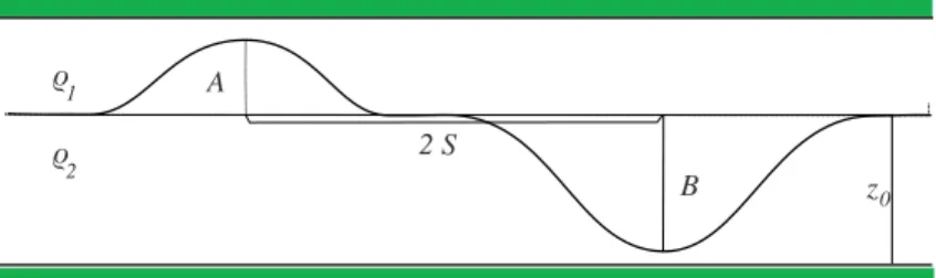
This formula allows explicit analytic computations for special cases. For instance, when the interface profile (see figure 2.4) is
η(x) = z0+Aexp
�
ρ1
ρ
2
B 2 S
A
z0
Figure 2.4: A two-bump configuration. Only when S is comparable with the typical width of the bumpsP∆ is nonzero.
the asymptotic difference of pressure is given by
P∆ ∼ 64
√ 3πg
81ρ1
S3e−8S2 3σ2
σ5 AB(A+B)ρ 2
∆+o(ρ
2
∆). (2.48)
Here, for long-wave asymptotic consistency, σ should be taken sufficiently large, andA
and B need to be such that the extrema of function (2.47) do not touch the channel boundary.
Some interesting conclusions can be extracted from (2.48). First, if A = −B the interface of the system becomes symmetric and, as always in these configurations,
P∆ = 0. Second, explicit dependence on the asymptotic height z0 does not appear in formula (2.48). However, notice that the ranges of A and B are constrained by the choice of z0 if the interface has to stay away from the channel boundaries. Thus, by choosing, e.g., A+B = k and B = z0−s (for given parameters k and s) we fix the maximum and the minimum of the interface leaving only z0 as a free variable. In this caseP∆ is a quadratic function of the interface heightz0 and the vertex of the parabola is at A = B. Third, the most interesting behaviour is related to the dependence on the separation parameter S. If the two bumps are well separated (S �σ), then P∆ is exponentially small. However, when the supports of the two bumps have an intersection (S�σ), then P∆ is nonzero to leading order O(ρ
2
2.4 Full Euler system: pressure jump at t=0 in the small ρ∆ asymptotic limit
We consider again the full Euler system for a two-layer fluid with zero initial velocity. As seen in Section 2.2.2, in this case the expansion in ρ∆ of the pressure imbalance starts with the quadratic term. We now compute this term explicitly. Throughout this section, unless otherwise stated, we will reference density to that of the lower fluid, so that ρ2 = 1.
2.4.1 The small ρ∆ expansion
Consider an initial condition for the two-fluid stratification such as the one depicted in figure 2.1. Let the initial velocity be identically zero, with the fluid in hydrostatic equilibrium as|x| → ∞. In this case, the Euler equations (2.1) determine the pressure
p(x, z) at time t = 0 through the solution of the elliptic equation
∇ · �
1
ρ∇p
�
= 0 (2.49)
subject to the Neumann boundary conditions
∂p
∂x →0 as |x| → ∞,
∂p
∂z =−gρ at z= 0, h . (2.50)
Of course, non-differentiability of the density distribution for the case of figure 2.1 requires an appropriate interpretation of equation (2.49). We will enforce (2.49) sepa-rately in each of theρ1 and ρ2 domains, Ω1 and Ω2 say,
∇2p= 0, (x, z)∈Ω
so thatpis harmonic in each subdomain, and assign boundary conditions at the discon-tinuities ofρ. These consist of continuity of peverywhere, while its normal derivatives jump according to the “flux-continuity” condition
1 ρ1 ∂p ∂n � � � � 1 = 1 ρ2 ∂p ∂n � � � � 2 , (2.51)
with obvious meaning of the notation.
Let the variable density be defined as a perturbation away from a uniform density fluid
ρ=ρ2−�r(x, z), 0< ��1, (2.52)
whererpositive, so thatρ2is the maximum density of fluid. For notational convenience, we further choose units in such a way that h = 1, and g = 1. We seek a solution for the pressure equation as an asymptotic expansion
p=p(0)+�p(1)+�2p(2)+o(�2) (2.53)
whence, equating like-powers of�,
∇2p(0) = 0, ∇2p(1)+∇ ·(r∇p(0)) = 0, ∇2p(2)+∇ ·(r∇p(1)) +∇ ·(r2∇p(0)) = 0, . . .
(2.54) with boundary conditions, respectively,
∂p(0) ∂z � � � �
z=0,1
=−1, ∂p (1) ∂z � � � �
z=0,1
= r|z=0,1 ,
∂p(2) ∂z � � � �
z=0,1
= 0,
∂p(k)
∂x →0 as |x| → ∞ for k ≥0.
(2.55)
for p(1) in the form
∇2p(1) =r
z.
Since the system is two-layer, still denoting the usual Heaviside function asH, we have
r(x, z) = H(z−η(x)),
where the interface location z =η(x) behaves as
η(x)→z± as x→ ±∞, 0< η(x)<1.
This means that the heavy fluid density isρ2 = 1 and the light fluid density isρ1 = 1−�, so that, in the chosen units, ρ∆ =�. Let
p(1) =p(1)h + (z−z0)H(z−z0), (2.56)
where z0 is any reference height. The summand (z −z0)H(z −z0) takes care of the top and bottom boundary conditions, leaving a homogeneous Neumann problem for
p(1)h (x, z) in the infinite strip. The equation for p(1)h (x, z) is then
∇2p(1)h =δ(z−η(x))−δ(z−z0). (2.57)
To solve this we can make use of the identity
∞
�
n=1
cos(nπθ) =−1
2+δp(θ)≡ − 1 2 +
+∞
�
k=−∞
from the theory of distributions (Gelfand & Shilov, 1964). Indeed, we have
2
∞
�
n=1
cos(nπz) cos(nπη) =
∞
�
n=1
�
cos�nπ(z−η)�+ cos�nπ(z+η)��
=−1 +δp(z−η) +δp(z+η) = −1 +δ(z−η)
since 0< z < 1 and 0 < η < 1, so that the support of the second Dirac-δ always falls outside the channel. For the same reason the periodic shifts can be ignored for the first
δ. Hence, we are lead to the following expression of the right-hand side of (2.57):
δ(z−η(x))−δ(z−z0) = 2
∞
�
n=1
cos(nπz)(cos(nπη(x))−cos(nπz0)), (2.58)
from which, taking the homogeneous Neumann boundary conditions into account, the coefficient of the Fourier series expression ofp(1)h (x, z) can be read off. Indeed,
p(1)h (x, z) =
∞
�
n=0
an(x) cos(nπz) (2.59)
yields
a��n−n2π2a
n = 2(cos(nπη(x))−cos(nπz0)) for n≥0.
Forn = 0, a��
0 = 0⇔a0 = constant, say a0 = 0.For n > 0, the equation for an can be
solved by use of the Green function for the operator ∂2
x−n2π2 on the real line,
Gn(x, ξ) = −
1 2nπe
−nπ|x−ξ|,
to finally obtain
p(1)h (x, z) = � +∞
−∞ ∞
�
n=1
e−nπ|x−ξ|
nπ cos(nπz)
�
This expression shows that the layer-average of p(1)h is always zero at any fixed x -location, as integration of cos(nπz) vanishes for alln. Since the average of p(0) and the
component (z−z0)H(z−z0) of (2.56) is the same for any fixedx, we can conclude that no contribution to the average pressure differential �p(+∞)� − �p(−∞)� can arise at order�, as expected from the results of § 2.2.2, and the fact that, for equal asymptotic interfacial heights, the average and interface pressure imbalances are equal.
Next, we work on the second order pressure contributionp(2). We concentrate only
on the layer-average of the boundary term ∂xp(2) instead of the exact z-dependence.
Multiplying the p(2) equation by x, integrating over the fluid volume and taking into
account the boundary conditions yields
lim
L→∞
� 1
0
�
p(2)(L, z)−p(2)(−L, z)�dz =− lim
L→∞
�
[−L,+L]×[0,1]
r ∂xp(1)dxdz.
The top and bottom boundary contributions cancel out exactly from the p(1)h and p(2)
terms. Passing to the limit we retrieve a close relative of the general formula for the pressure differential in an infinite strip,
�p(2)�∆ ≡
� 1
0
�
p(2)(∞, z)−p(2)(−∞, z)�dz =− �
R×[0,1]
r ∂xp(1)dxdz. (2.61)
Substituting expression (2.60) forp(1)h yields
�p(2)�∆=− � +∞
−∞
�� +∞
−∞
sgn(x−ξ)
∞
�
n=1
e−nπ|x−ξ|(cos(nπη(ξ))−cos(nπz0)) dξ
× � 1
0
cos(nπz)H(z−η(x)) dz
� dx .
(2.62)
The last integral is
� 1
η(x)
cos(nπz) dz=− 1
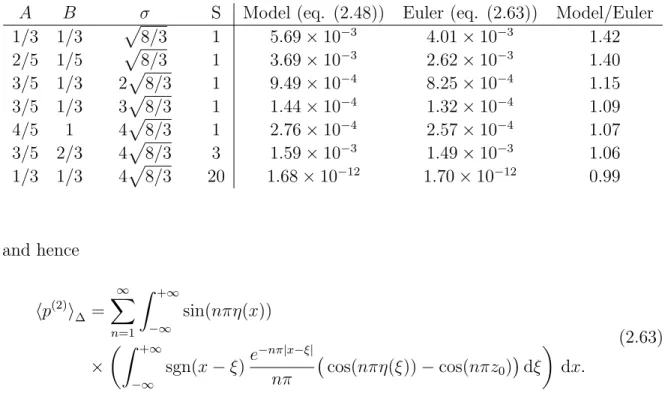
Table 2.1: Comparison of pressure imbalances P∆/ρ2
∆ as predicted by long-wave model and full Euler results for interface (2.47) with asymptotic height z0 = 1/2.
A B σ S Model (eq. (2.48)) Euler (eq. (2.63)) Model/Euler 1/3 1/3 �8/3 1 5.69×10⁻³ 4.01×10⁻³ 1.42
2/5 1/5 �8/3 1 3.69×10⁻³ 2.62×10⁻³ 1.40
3/5 1/3 2�8/3 1 9.49×10⁻⁴ 8.25×10⁻⁴ 1.15
3/5 1/3 3�8/3 1 1.44×10⁻⁴ 1.32×10⁻⁴ 1.09
4/5 1 4�8/3 1 2.76×10⁻⁴ 2.57×10⁻⁴ 1.07
3/5 2/3 4�8/3 3 1.59×10⁻³ 1.49×10⁻³ 1.06
1/3 1/3 4�8/3 20 1.68×10⁻¹² 1.70×10⁻¹² 0.99
and hence
�p(2)�∆=
∞
�
n=1
� +∞
−∞
sin(nπη(x))
×
�� +∞
−∞
sgn(x−ξ)e
−nπ|x−ξ|
nπ
�
cos(nπη(ξ))−cos(nπz0)�dξ
� dx.
(2.63)
We remark that all the theoretical arguments for the determination of the pressure jump �p(2)�
∆ have assumed that the interface does not touch the channel boundaries.
Thus, there are always slivers of light and heavy fluid near the top and bottom lid, respectively. However, it is not difficult to realize that, since all integrals are bounded, and the integrands decay exponentially, we can pass to the limit of zero sliver-width in the above formulae. Furthermore, since p(2) is no longer affected by the density
2.4.2 Comparison with the long wave model
Expression (2.63) can be used to test the long-wave model result (2.46) with, e.g.,
η(x) given by (2.47). While we are unable to compute the integrals in (2.63) explicitly, their numerical evaluation for up to 25 terms in the series yields agreement over a broad range of parameters. Table 2.1 reports a few examples. For these, the long wave model pressure imbalance (2.46) is always of the same order of its Euler counterpart (2.63), with the discrepancy decreasing as the main long wave parameterσincreases. Remark-ably, the agreement is acceptable already for σ= 3�8/3�4.9, which for a channel of height h = 1 would correspond to a value of the long-wave small parameter δ � 0.2. The trend exemplified by table 2.1 persists in general for all the parameter combinations we have checked.
We note that the convergence of the series in (2.63) is slow for the class of smooth profiles from (2.47) we have explored, which partially adds to the discrepancy in ta-ble 2.1. A general convergence proof and an estimate of the convergence rate shows that the series coefficients are bounded by 1/n2, for any interface functionηof bounded
variation class. Next, we focus instead on special profiles where the series summation can be performed explicitly.
2.4.3 Special initial conditions: piecewise-constant interfaces
Let us consider the integral formula (2.63) for a profile η that is smooth on the whole line, except possibly at a finite number of points A1, A2, . . . , AN, where the
jumps η(A+
α)−η(A−α) are finite. We also require, as usual, that limx→±∞η(x) =z± for
some asymptotic valuesz±. Taking into account the distributional identity
sgn(x−ξ)e−nπ|x−ξ|= 1
nπ d dξe
integrating by parts, and considering the distributional derivative of cos(nπη(ξ)), leads to an expression equivalent to (2.63),
�p(2)�∆=
∞ � n=1 1 nπ � +∞ −∞
sin(nπη(x))
�� +∞
−∞
e−nπ|x−ξ|η�(ξ) sin(nπη(ξ)) dξ
� dx − ∞ � n=1 1
n2π2
N
�
α=1
� +∞
−∞
dxsin(nπη(x))e−nπ|x−Aα|�cos(nπη(A−
α))−cos(nπη(A+α))
� dx.
(2.64)
Now, for piecewise-constant interface profiles
η(ξ) =zi for Ai < ξ < Ai+1, i= 1, . . . , N −1,
η(ξ) =z− ≡z0 for ξ < A1 and η(ξ) =z+ ≡zN for ξ > AN,
(2.65)
only the second line of equation (2.64) provides a contribution, and we have η(A−α) =
zα−1, η(A+α) =zα.
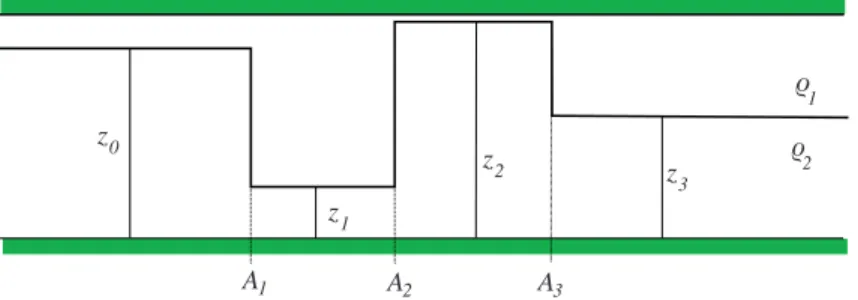
Because of the shape achieved by each fluid’s domain in the limiting three step case withz1 = 0 andz2 = 1, i.e., disconnected domains with no connecting slivers at the top
and bottom plates, in what follows we will often refer to this class of initial conditions as “hooks,” see figure 2.5. We remark that these are possibly the simplest configurations yielding explicit expressions for non-vanishing pressure imbalances. Moreover, hooks can in principle be implemented experimentally by use of gates separating the fluids, just as in the limiting configuration of the dam-break case (corresponding to z0 = 0,
z3 = 1, z1 = z2 = 0, all A’s zero) with a single gate spanning the whole width of the
channel. Performing the integrations in (2.64) we get that the pressure jump at the second order in the ρ∆ expansion is given by
�p(2)� ∆=
∞
�
k=1
1
π3k3
�
∆(0k)+ �
1≤α<β≤N
∆([α,βk) ]ekπ(Aα−Aβ) �
ρ1
ρ
2
z0
z1
z2 z
3
A2 A3 A1
Figure 2.5: Initial hook-like configuration for a two-fluid density distribution in an
x-infinite channel between two rigid plates located atz = 0,1.
where
∆(0k)=
N
�
α=1
sin(kπ(zα−zα−1)) +
1
2(sin(2kπ z0)−sin(2kπ zN)), (2.67)
and
∆([α,βk) ]= (cos(kπ zβ)−cos(kπ zβ−1))(sin(kπ zα)−sin(kπ zα−1)+
−(cos(kπ zα)−cos(kπ zα−1))(sin(kπ zβ)−sin(kπ zβ−1)),
(2.68)
or, equivalently,
∆([α,βk) ]= sin(kπ(zα−zβ))−sin(kπ(zα−1−zβ))+
−sin(kπ(zα−zβ−1)) + sin(kπ(zα−1−zβ−1)).
(2.69)
In particular, for the ‘three-jump’ case, with discontinuities located at A1 ≤ A2 ≤ A3
and arbitrary heights 0≤z0, z1, z2 ≤1,z0 =z3, we have
�p(2)�∆=
∞
�
k=1
1
π3k3
�
(sin(kπ(z1−z0)) + sin(kπ(z2−z1)) + sin(kπ(z0−z2)))
×�1−ekπ(A1−A2)� �1−ekπ(A2−A3)� �.
(2.70)