MODEL ASSESSMENT FOR MODELS WITH MISSING DATA
Xiaolei Zhou
A dissertation submitted to the faculty of the University of North Carolina at Chapel Hill in partial fulfillment of the requirements for the degree of Doctor of Philosophy in the Department of Biostatistics in the Gillings School of Global Public Health.
Chapel Hill 2015
Approved by: Hongtu Zhu Elizabeth Andrews Shrikant Bangdiwala Yun Li
ABSTRACT
Xiaolei Zhou: Model Assessment for Models with Missing Data (Under the direction of Hongtu Zhu)
Missing data commonly occur in various study setting. In this dissertation, we first investigate three likelihood-based models for missing data in longitudinal studies: mixed effects models, pattern mixture models (PMM), and selection models. Extensive simulations from ten missing mechanisms are performed with the focus on treatment effect. Results suggest that no model consistently performs better than others under various missing data mechanism. However, PMM using the treatment-specific proportion and selection model provide some correction of the estimate compared with mixed-effects model in several missing not at random situations, even when the mechanism of missing data is not exactly the same as the model assumption.
matters issue in GLM with missing covariates. The applications of scaled Cook's distances in a formal influence analysis are examined in simulations and real data examples.
At last, we examine the connection between case deletion measures and cross validation method for GLM with missing covariates models. Based on such connection, we develop case-deletion model complexity (CMC) measures for quantifying the model complexity and case-deletion information criteria (CIC) for model selection. We develop these new measures and criteria based on the likelihood function and the Q-function, respectively. Some
ACKNOWLEDGMENTS
TABLE OF CONTENTS
LIST OF TABLES . . . .ix
LIST OF FIGURES . . . x
CHAPTER 1: INTRODUCTION . . . 1
1.1 Missing Data and Treatment Effect . . . 2
1.2 Model Assessment . . . .5
1.2.1 Case Influence Measures . . . .6
1.2.2 Criterion-based Model Assessment . . . .9
CHAPTER 2: COMPARISON OF STATISTICAL MODELS IN ESTIMATING TREATMENT EFFECT FOR MISSING DATA IN LONGITUDINAL STUDIES . . . 11
2.1 Introduction . . . .11
2.2 Treatment Effect . . . 12
2.3 Existing Methods . . . .15
2.3.1 Mixed-effects Models . . . 16
2.3.2 Pattern-mixture Models . . . .18
2.3.3 Selection Models . . . 19
2.4 Simulation . . . .. . . 20
2.4.1 Data Generation . . . 20
2.4.2 Analysis of the Simulated Data. . . .24
2.6 Conclusions. . . 31
CHAPTER 3: DIAGNOSTIC MEASURES FOR GENERALIZED LINEAR MODELS WITH MISSING COVARIATES. . . .32
3.1 Introduction. . . 32
3.2 Generalized Linear Model with Missing Covariate Data . . . 33
3.3 Degree of Perturbation . . . 39
3.4 Cook's Distance. . . 44
3.5 Scaled Cook's Distance. . . 50
3.6 Simulation Studies Using One Dataset. . . 51
3.7 Additional Simulation Studies. . . 67
3.8 Real Data Examples . . . 78
3.8.1 National Survey Cholesterol Data. . . 78
3.8.2 Liver Cancer Data . . . 79
3.9 Conclusions. . . 80
CHAPTER 4: INFORMATION CRITERIA FOR GENERALIZED LINEAR MODELS WITH MISSING COVARIATES . . . 82
4.1 Introduction . . . .82
4.2 Method. . . 83
4.2.1 Case Deletion Measures. . . 83
4.2.2 Cross Validation and Model Complexity . . . 84
4.2.3 Case-deletion Information Criterion . . . 86
4.3 Simulation. . . 87
4.4 Real Data Analysis . . . 91
LIST OF TABLES
2.1 Treatment Effect for Four Commonly Used Models . . . 13 2.2 Examples of Mixed-effects Models, PMMs, and Selection Models . . . 17 2.3 Missing Data Mechanism and Missing Rate in Simulation Data . . . .22 2.4 Average Treatment Effect and Its Standard Error Estimated from the
Mixed-Effects Model, the Pattern-Mixture Model, and the
Selection Model for Scenarios 1 to 6 (true treatment effect = 1) . . . 28 2.5 Average Treatment Effect and Its Standard Error Estimated from the
Mixed-Effects Model, the Pattern-Mixture Model, and the
Selection model for Scenarios 7 to 10. . . 29 3.1 Summary of Simulation Scenarios . . . 53 4.1 Comparison of Ranks of the True Model M1 from Various Model
Selection Criteria in GLM with Missing Covariates. . . 89 4.2 Comparison of Ranks for M1 to M5 from Various Model Selection
LIST OF FIGURES
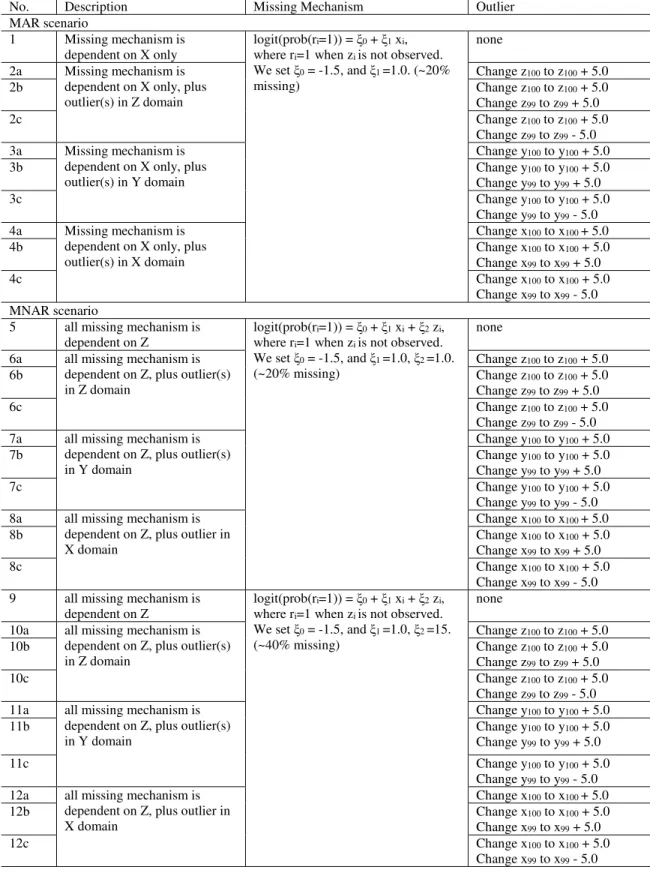
3.1 Index Plots and Scatter Plots of CD and QCD from the Simulation Data with No Outlier. The three plots in the top are from the scenario of MAR (Scenario 1). The three plots in the middle are from the scenario of MNAR (Scenario 5). The three plots in the bottom are from the scenario of MNAR with a greater
missing rate (Scenario 9) . . . 55 3.2 Index Plots and Scatter Plots of CD and QCD from the Simulation
Data with One Outlier in z Domain. The three plots in the top are from the scenario of MAR (Scenario 2a). The three plots in the middle are from the scenario of MNAR (Scenario 6a). The three plots in the bottom are from the scenario of MNAR with
a greater missing rate (Scenario 10a). . . .57 3.3 Index Plots and Scatter Plots of CD and QCD from the Simulation
Data with Two Outliers in z Domain in Same Direction. The three plots in the top are from the scenario of MAR (Scenario 2b). The three plots in the middle are from the scenario of MNAR (Scenario 6b). The three plots in the bottom are from the scenario
of MNAR with a greater missing rate (Scenario 10b). . . 58 3.4 Index Plots and Scatter Plots of CD and QCD from the Simulation
Data with Two Outliers in z Domain in Opposite Direction. The three plots in the top are from the scenario of MAR (Scenario 2c). The three plots in the middle are from the scenario of MNAR (Scenario 6c). The three plots in the bottom are from the scenario
of MNAR with a greater missing rate (Scenario 10c). . . 59 3.5 Index Plots and Scatter Plots of CD and QCD from the Simulation
Data with One Outlier in y Domain. The three plots in the top are from the scenario of MAR (Scenario 3a). The three plots in the middle are from the scenario of MNAR (Scenario 7a). The three plots in the bottom are from the scenario of MNAR with a
greater missing rate (Scenario 11a) . . . 60 3.6 Index Plots and Scatter Plots of CD and QCD from the Simulation
Data with Two Outliers in y Domain in Same Direction. The three plots in the top are from the scenario of MAR (Scenario 3b). The three plots in the middle are from the scenario of MNAR (Scenario 7b). The three plots in the bottom are from the scenario
3.7 Index Plots and Scatter Plots of CD and QCD from the Simulation Data with Two Outliers in y Domain in Opposite Direction. The three plots in the top are from the scenario of MAR (Scenario 3c). The three plots in the middle are from the scenario of MNAR (Scenario 7c). The three plots in the bottom are from the scenario
of MNAR with a greater missing rate (Scenario 11c). . . 62 3.8 Index Plots and Scatter Plots of CD and QCD from the Simulation Data
with One Outlier in x Domain. The three plots in the top are from the scenario of MAR (Scenario 4a). The three plots in the middle are from the scenario of MNAR (Scenario 8a). The three plots in the bottom are from the scenario of MNAR with a greater missing
rate (Scenario 12a). . . 64 3.9 Index Plots and Scatter Plots of CD and QCD from the Simulation Data
with Two Outliers in x Domain in Same Direction. The three plots in the top are from the scenario of MAR (Scenario 4b). The three plots in the middle are from the scenario of MNAR (Scenario 8b). The three plots in the bottom are from the scenario of MNAR with
a greater missing rate (Scenario 12b) . . . 65 3.10 Index Plots and Scatter Plots of CD and QCD from the Simulation
Data with Two Outliers in x Domain in Opposite Direction. The three plots in the top are from the scenario of MAR (Scenario 4c). The three plots in the middle are from the scenario of MNAR (Scenario 8c). The three plots in the bottom are from the scenario
of MNAR with a greater missing rate (Scenario 12c). . . 66 3.11 Box Plots for CD, Scaled CD, Pr and Scatter Plots with Q-based
Approximation. Results from 100 Simulation Samples for Scenario 1. Green dots indicates means. Red bars (dots) are
observed, and blue bars (dots) are subjects with missing z. . . 68 3.12 Scatter Plots of Mean Degree of Perturbation with x, Mean CD,
and Mean Scaled CD. Results from 100 Simulation Samples for Scenario 1. Red dots are observed subjects, and blue dots
are subjects with missing z . . . 69 3.13 Box Plots for CD, Scaled CD, and Pr. Results from 100 Simulation
Samples for Scenarios 2a (MAR, left panels) and 6a (MNAR, right panels) - 5 Outliers in z Domain in the Same Direction. Green dots indicates means. Red bars (dots) are observed, and
3.14 Box Plots for CD, Scaled CD, and Pr. Results from 100 Simulation Samples for Scenarios 2b (MAR, left panels) and 6b (MNAR, right panels) - 5 Outliers in z Domain in the Opposite Direction. Green dots indicates means. Red bars (dots) are observed, and
blue bars (dots) are subjects with missing z . . . 72 3.15 Box Plots for CD, Scaled CD, and Pr. Results from 100 Simulation
Samples for Scenarios 3a (MAR, left panels) and 7a (MNAR, right panels) - 5 Outliers in y Domain in the Same Direction. Green dots indicates means. Red bars (dots) are observed, and
blue bars (dots) are subjects with missing z . . . 74 3.16 Box Plots for CD, Scaled CD, and Pr. Results from 100 Simulation
Samples for Scenarios 3b (MAR, left panels) and 7b (MNAR, right panels) - 5 Outliers in y Domain in the Opposite Direction. Green dots indicates means. Red bars (dots) are observed, and
blue bars (dots) are subjects with missing z . . . 75 3.17 Box Plots for CD, Scaled CD, and Pr. Results from 100 Simulation
Samples for Scenarios 4a (MAR, left panels) and 8a (MNAR, right panels) - 5 Outliers in x Domain in the Same Direction. Green dots indicates means. Red bars (dots) are observed, and
blue bars (dots) are subjects with missing z . . . 76 3.18 Box Plots for CD, Scaled CD, and Pr. Results from 100 Simulation
Samples for Scenarios 4b (MAR, left panels) and 8b (MNAR, right panels) - 5 Outliers in x Domain in the Opposite Direction. Green dots indicates means. Red bars (dots) are observed, and
CHAPTER 1
INTRODUCTION
In the “big data” era, a large amount of data is available and waiting for people to
find out what is hidden inside. These data may come from a “true” complicated process.
Statisticians use statistical models to interpret data and to approximate the true
compli-cate process. However, the fitted model is nearly always not the true process. How to use
statistical tools (diagnostic measures) to detect the discrepancies between fitted model
and true process is a very important question for statisticians. We can distinguish two
types of discrepancies: i) discrepancy existing between isolated observations (influential
points and outliers) and the rest of the observations, and ii) systematic discrepancies
between the data and the fitted value obtained from statistical models. The existence of
missing data further increases the complexity of model fitting and diagnosis. Although
several methods have been developed to handle missing data, it remains a challenging
and active field for statisticians.
In this dissertation, we first present literature reviews. Then in Chapter 2, we compare
mixed-effects model, pattern-mixture model, and selection model in estimating treatment
effect for missing data in longitudinal studies. In Chapter 3, we develop the scaled Cook’s
distance for generalized linear models with missing covariates. In Chapter 4, we develop
the case-deletion information criterion for model selection on generalized linear models
1.1 Missing Data and Treatment Effect
Missing data commonly occur in longitudinal studies. In clinical trial studies,
patient-reported outcomes (PROs), such as health-related quality of life (HRQOL) and symptoms
collected via validated questionnaires, often have a higher missing rate compared with
clinical outcomes evaluated by physicians. In some severe diseases, such as metastatic
breast cancer, it is not uncommon for 15% of patients to be missing HRQOL data even
at baseline (Zhou et al., 2009). Additional missingness occurring after baseline further
reduces the proportion of patients with data available for analysis. The reasons for
and amount of missing HRQOL data in clinical trials depend on the disease and when
and how the study is conducted and may not be similar among different treatment
groups. Fairclough (2010) listed various reasons why subjects fail to complete HRQOL
assessments. Some missing data may be caused by administrative reasons, such as staff
forgetting to administer the questionnaire or translation not available in the patient’s
language. The missing value may also be related to the patient’s condition; for example,
the patient stated that he or she was too ill to complete the questionnaire. The high
missing rate in HRQOL data can also be caused by a self-assessment questionnaire that
contains a long series of questions. Once a patient has missed an HRQOL assessment,
the retrospective collection of these data is usually impossible.
It is well known that missing data may not only reduce the power to detect change
from baseline but, more important, will lead to biased estimates of response when
miss-ingness depends on the response. At the end of 2009, the Food and Drug Administration
(FDA, 2009) published a guidance for industry in using PROs in clinical trials for label
claims. The guidance encourages the study to minimize patients’ dropouts and collect
PRO data even after patients have discontinued treatment. The study’s protocol and
statistical analysis plan should describe how missing data will be handled in the analysis.
statisti-cal strategies to deal with missing data due to early termination of patients before the
planned completion of a trial. European Medicines Agency (2010) guideline on missing
data in confirmatory clinical trials concur with this.
In 2010, the Panel on the Handling of Missing Data in Clinical Trials under the
National Research Council (2010) published a report with recommendations that will be
used not only to the FDA but also to the entire clinical trial community (Little et al.,
2012, O’Neill and Temple, 2012). The panel classified four types of approaches to adjust
for missing data: complete-case analysis (excluding subjects with missing data from
analysis), single imputation methods (such as last observation carried forward or baseline
value carried forward, was used in some clinical trials), estimating-equation methods, and
methods based on a statistical model. In estimating-equation methods, complete cases
are weighted by the inverse of an estimate of the probability of being observed, which may
be modeled with the use of observed variables, for example, baseline data. The statistical
model based methods includes likelihood function-based models, Bayesian methods, and
multiple imputation.
For the missing data problem, the applicability of the different methods is based
on a classification of the following missingness mechanisms: missing completely at
ran-dom (MCAR), missing at ranran-dom (MAR), and missing not at ranran-dom (MNAR). If the
probability of an observation being missing does not depend on observed or unobserved
measurements, then the observation is MCAR. If the probability of an observation
be-ing missbe-ing depends only on observed measurements, then the observation is MAR. If
the probability of an observation being missing depends on unobserved measurements
(e.g., patients with a poor outcome score are more likely to miss the assessment), then
the observation is MNAR. This type of missing data is also called nonignorable missing
data.
Complete-case analysis is based on MCAR. Single imputation methods is arbitrary.
but they are built on ignorable missingness or MAR (Little et al., 2012, Ali and Siddiqui,
2000). The mixed-effects model, as a likelihood function-based model, is a frequent
choice for analyzing continuous outcomes in clinical trials because it uses all available
observed data and are valid when missing data are MCAR or MAR. However, when
missing data depend on an unobserved outcome (MNAR), the parameter estimates from
the mixed-effects model can be biased.
In clinical trial studies, we cannot rule out the MNAR scenario and sometimes it may
be more realistic than MAR; thus, it is recommended to assess the robustness of the
results by performing sensitivity analysis under the assumption of MNAR. Development
of statistical methods to handle MNAR data is a very important and promising area.
Ibrahim and colleagues (2005) and Ibrahim and Molenberghs (2009) provided several
overview articles of various models for missing data problems. Pattern-mixture model
(PMM) and selection model are two major methods to handle missing data under MNAR
based on likelihood functions. To account for nonignorable missing data, in addition to
random variables in the mixed-effects model, PMM and selection model include an
ad-ditional random variable for missingness in the likelihood functions (missing pattern in
PMM and missingness indicator in selection model). In both models, the random variable
for missing mechanism is not independent with the response variable. Pattern-mixture
models (Little, 1995) have been used widely to analyze continuous PRO data. A popular
PPM for PRO data analysis assumes that the missing mechanism depends only on
treat-ment (Hedeker and Gibbons, 1997). Pauler and colleagues (2003) further provided details
on how to estimate overall treatment effect from pattern-specific estimates based on the
treatment-specific proportion of the pattern when HRQOL changes linearly over time.
The missing mechanism may also depend on other covariates or response. The selection
model is based on the assumption of MNAR that whether or not the dependent variable
is missing depends directly on the value of the dependent variable at the time of missing.
expectation-maximization (MCEM) algorithm (Ibrahim et al., 2001, 2005, Ibrahim and Molenberghs,
2009). Both PMM and selection model have been applied using the Bayesian approach
(Daniels and Hogan, 2008, Little et al., 2011). Note that the pattern-mixture model and
selection model factorizations of the likelihood functions can be used to develop more
complex methods of joint modeling of responses and missing data process such as the
shared-parameter models (Ibrahim and Molenberghs, 2009, Daniels and Hogan, 2008),
where the missingness may depend on the random effect.
All models for handling missing data under MNAR make specific assumptions, which
are often untestable, and the statistical results obtained from different MNAR models
can be different. Therefore, the models under MNAR are often considered as part of a
sensitivity analysis (Molenberghs et al., 2001, 2004, Verbeke et al., 2001b). Although it
is well known that the estimates of response obtained from mixed-effects models fitted
to MNAR missing data can be biased, the impact of missing data on the estimate of
treatment effect (the difference between treatments) is more complex, depending on the
proportion of and reason for missing data in all treatment groups. Several studies (Pauler
et al., 2003, Michiels et al., 2002, Post et al., 2010) have included treatment effects
estimated from mixed-effects model and PMM or selection model using collected data.
However, because the true treatment effect is unknown in collected data, it is impossible
to evaluate the bias of the estimate using collected data. A simulation study is needed
to evaluate the impact of missing data on the estimate of treatment effect.
1.2 Model Assessment
The goal of the diagnostic measures is to assess how well the model fits the data and
how robust it is. Residuals (the difference between the observed response and the
model-predicted response) provide very important information about the model fitting, not only
for the individual observations, but also for the global model fitting. Instead of comparing
influence measure. If a minor modification of the model seriously influences key results
of an analysis, it will be a cause for concern. On the other hand, if such modifications
do not have large impact the results, the model is robust with respect to the induced
perturbations (Cook, 1986).
1.2.1 Case Influence Measures
Case deletion measures assess the influence of deleting one or a set of observations from
the data on certain statistics. They are often used to identify influential points or the
impact of one or a few observations on overall model fitting. Two widely used case
deletion measures are Cook’s distance (Cook, 1977) and likelihood displacement (Cook
and Weisberg, 1982, Cook, 1986). The likelihood displacement measures the difference in
log-likelihood when one or a set of observations are removed. The likelihood displacement
is defined by
LD(i) = 2[l(ˆθ)−l(ˆθ[i])],
where θ is a pvector of the parameter of interest, ˆθ is the parameter estimated with full
data, ˆθ[i] is the parameter estimates using data with the ith case deleted, andl(θ) is the
log-likelihood function forθ. The Cook’s distance measures the impact of deleting one or
a set of observations on parameter estimates. The generalized Cook’s distance is defined
by
CD(i) = (ˆθ[i]−θˆ)>G(ˆθ[i]−θˆ),
where G is a positive definite matrix, e.g., −∂θ2l(ˆθ). It has been shown that Cook’s
dis-tance combines information from the studentized residuals and the variance of predicted
values for general linear model (Cook, 1977).
Most of the diagnostic measures were originally developed under linear regression
models (Cook, 1977, Cook and Weisberg, 1982, Chatterjee and Hadi, 1986), and then
1992), generalized estimating equations (Preisser and Qaqish, 1996), models for clustered
data(Christensen et al., 1992, Banerjee and Frees, 1997, Haslett and Dillane, 2004), and
survival data (Weissfeld, 1990, Lin et al., 1993). In addition, considerable research has
been conducted to develop case influence measures in Bayesian analysis (Johnson and
Geisser, 1983, 1985, Pettit, 1986, Carlin and Carlin, 1991, Gelfand et al., 1992, Weiss
and Cook, 1992, Blyth, 1994, Peng and Dey, 1995, Weiss, 1996, Bradlow and Zaslavsky,
1997). Zhu et al. (2010) provided a comprehensive review of various Bayesian case
in-fluence measures and their properties. In Bayesian analysis, the inin-fluence of individual
observations (or a set of observations) is often assessed by comparing the posterior (or
predictive) distribution of the full data to the distribution after deleting these
obser-vations (case deletion). For example, the Cook’s posterior mode distance, denoted by
CP(i), quantifies the discrepancy between the posterior mode of θ with and without the
ith case (Cook and Weisberg, 1982). The posterior modes ofθ for the full sample Y and
a subsample Y[i] are defined as ˆθ = argmaxθlogp(θ|Y) and ˆθ[i] = argmaxθlogp(θ|Y[i]),
respectively. CP(i) is given by
CP(i) = (ˆθ[i]−θˆ)>Gθ(ˆθ[i]−θˆ),
whereGθis chosen to be a positive definite matrix. For instance,Gθcan be −∂θ2logp(θ|Y)
=−∂2
θlogp(Y|θ)−∂θ2logp(θ) evaluated at ˆθ. Similarly, the Cook’s posterior mean
dis-tance, denoted by CM(i), quantifies the discrepancy between the posterior mean of θ
with and without theith case. The posterior means ofθ for the full sampleY and a
sub-sample Y[i] are defined as ˜θ =
R
θp(θ|Y)dθ and ˜θ[i] =
R
θp˙(θ|Y[i])dθ, respectively. CM(i)
is given by
CM(i) = (˜θ[i]−θ˜)>Wθ(˜θ[i]−θ˜),
where Wθ is chosen to be a positive definite matrix.
et al., 2001, 2009, 2012b). The models for missing data usually use the EM algorithm
to obtain the maximum likelihood estimates (Lipsitz and Ibrahim, 1996, Ibrahim et al.,
1999). In EM algorithm, the MLE of the parametersθin the complete likelihood function
(based on complete data) is obtained through iterations that maximizes the Q-function
Q(θ|θˆ) = E[lc(θ|Dc)|Do,θˆ],
where Dc being the complete data, Do being the observed data, and lc(θ|Dc) is the
complete-data log-likelihood function. Zhu et al. (2001) used Q-function to replace the
log likelihood in the likelihood displacement and showed that the analytic results were
very similar to those obtained from a classical local influence approach based on the
observed data likelihood function. Q-function is also used to obtain Cook’s distance for
generalized linear model with missing covariates (Zhu et al., 2009). However, to our
knowledge, there is no literature to assess how close the Cook’s distance obtained from
the Q-function compares to that obtained from the classical likelihood function.
Cook’s distance is one of the most important diagnostic tools. A large value of
Cook’s distance indicates that the observation is influential. However, Zhu et al. (2012a)
deliberated size matters issue of Cook’s distance. Cook’s distance may not be directly
comparable because the scale of Cook’s distance stochastically depends on the degree of
the perturbation. Dr. Zhu et al. introduced the scaled Cook’s distance to detect the
relatively influential subjects in the sense that the Cook’s distance is large relative to the
degree of perturbation. How the missing data impacts the degree of perturbation has
not been evaluated.
In addition to case deletion measures, a broader range of sensitive analyses have been
developed to assess the robustness of a model when perturbing the model assumptions
and/or individual observations. In frequentist analysis, extensive literature exists on
and Rubin, 2002, Verbeke et al., 2001a, van Steen et al., 2001, Jansen et al., 2003,
2006, Copas and Eguchi, 2005, Daniels and Hogan, 2008, Shi et al., 2009). The general
questions are how to introduce an appropriate perturbation and how to assess its influence
on a model. In the Bayesian analysis of statistical models with missing data, Zhu et al.
(2014b) in their recent paper introduced various perturbations to modeling assumptions
and individual observations, and then developed a formal sensitivity analysis to assess
theses perturbations.
1.2.2 Criterion-based Model Assessment
To select an optimal model from a pool of statistical models for a given dataset, we
often need to consider both goodness of fit and model complexity. A model which
bal-ances model fitting and complexity is preferred. To achieve this, various information
criteria have been proposed for model comparisons, which incorporate measures of fit
and complexity for model choice. Such information criteria include Akaiki Information
Criterion (AIC) (Akaike, 1974), Takeuchi Information Criterion (TIC) (Takeuchi, 1976),
Generalized Information Criterion (GIC), (Konishi and Kitagawa, 1996), Network
Infor-mation Criterion (NIC) (Murata et al., 1994) the Bayesian InforInfor-mation Criterion (BIC)
(Schwarz et al., 1978, Lv and Liu, 2014, Konishi et al., 2004), the Deviance Information
Criterion (DIC) (Spiegelhalter et al., 2002), Bayesian Predictive Information Criterion
(BPIC) (Ando, 2007), and many others. In these criteria, the goodness of fit are based on
the deviance component −2 logp(y|θˆ) or the posterior mean of the deviance component
−2Eθ|ylogp(y|θ), while the measures of model complexity vary from simply the number
of parameters to more complicated form. (Ibrahim et al., 2008) Recently, Zhu et al.
(2014a) proposed a set of Bayesian case-deletion model complexity measure to quantify
the effective number of parameters in a given statistical model, which leads to a Bayesian
case-deletion information criterion (BCIC) for model comparison.
including missing data, because these model selection criteria depend on the likelihood
function based on the observed data. Some research (Garcia et al., 2010, Ibrahim et al.,
2008) has been conducted to use the key components of the EM algorithm, such as the
CHAPTER 2
COMPARISON OF STATISTICAL MODELS IN ESTIMATING TREATMENT EFFECT FOR MISSING DATA IN LONGITUDINAL
STUDIES
2.1 Introduction
The aim of this chapter is to examine the magnitude of the bias and the robustness of
mixed-effects models, PMMs, and selection models under different MNAR mechanisms
that are at different degrees of perturbation to the model assumptions. Our primary
interest is on the estimate of treatment effect, which is the interest of most clinical trials
and many observational studies. We also perform sensitivity analyses and simulations
to evaluate the robustness of the PMM, selection model, and mixed-effects model on
the estimates of treatment effects. The methods discussed in this manuscript and the
simulations performed were motivated by the analysis of PROs. However, they are
ap-propriate for the broader problem of missing data. These analyses are the first we know
to systematically evaluate and compare the mixed-effects models, PMMs, and selection
models using simulation data.
Section 2.2 defines treatment effect, and Section 2.3 reviews the three existing
mod-els: mixed-effects models, PMMs, and selection models. In Section 2.4, we describe an
extensive simulation study on comparing the three statistical models under several
com-mon scenarios of missing-data mechanisms, focusing on the treatment effect. Results are
2.2 Treatment Effect
Treatment effect is the primary interest in clinical trials. A large amount of literature
has been developed regard the effect of treatments on HRQOL in various disease areas
(Zhou et al., 2009, Sherrill et al., 2010). Different analysis methods have been used to
evaluate the treatment effect on HRQOL. However, the statistical definition of treatment
effect is not always clear or correct, even in some published methods articles.
Depending on the structure of models, treatment effect can be obtained from different
regression coefficients. For continuous outcomes, there are two popular types of models
based on the form of outcome. One type directly uses the response score as the dependent
variable, whereas the other uses change from baseline score as the dependent variable.
These models can also be further classified based on whether baseline measure is included.
The baseline measure is the one assessed before treatment initiation. We denote this
time point as t = 0. Table 2.1 summarizes how to obtain the treatment effects for four
commonly used models. We define treatment effect as the difference in the expected
value of the response scores between treatments after accounting for baseline difference.
In models 1 and 2, baseline value is not included in the models as a covariate. Therefore,
the treatment effect is obtained by subtracting the baseline difference from the response
difference. In models 3 and 4, baseline difference is accounted for by including the baseline
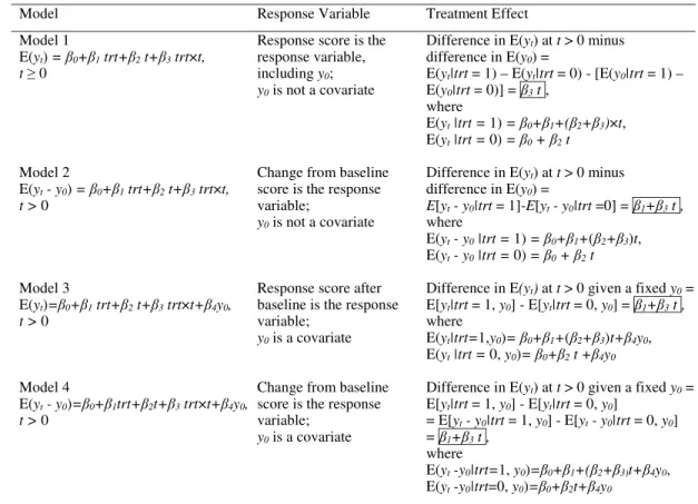
Table 2.1: Treatment Effect for Four Commonly Used Models
Model Response Variable Treatment Effect
Model 1
E(yt) = β0+β1 trt+β2 t+β3 trt×t, t ≥ 0
Response score is the response variable, including y0;
y0 is not a covariate
Difference in E(yt) at t > 0 minus difference in E(y0) =
E(yt|trt = 1) – E(yt|trt = 0) - [E(y0|trt = 1) – E(y0|trt = 0)] = β3 t ,
where
E(yt |trt = 1) = β0+β1+(β2+β3)×t, E(yt |trt = 0) = β0 + β2 t Model 2
E(yt - y0) = β0+β1 trt+β2 t+β3 trt×t, t > 0
Change from baseline score is the response variable;
y0 is not a covariate
Difference in E(yt) at t > 0 minus difference in E(y0) =
E[yt - y0|trt = 1]-E[yt - y0|trt =0] = β1+β3 t , where
E(yt - y0 |trt = 1) = β0+β1+(β2+β3)t, E(yt - y0 |trt = 0) = β0 + β2 t Model 3
E(yt)=β0+β1 trt+β2 t+β3 trt×t+β4y0, t > 0
Response score after baseline is the response variable;
y0 is a covariate
Difference in E(yt) at t > 0 given a fixed y0 = E[yt|trt = 1, y0] - E[yt|trt = 0, y0] = β1+β3 t , where
E(yt|trt=1,y0)= β0+β1+(β2+β3)t+β4y0, E(yt |trt = 0, y0)= β0+β2 t +β4y0 Model 4
E(yt - y0)=β0+β1trt+β2t+β3 trt×t+β4y0, t > 0
Change from baseline score is the response variable;
y0 is a covariate
Difference in E(yt) at t > 0 given a fixed y0 = E[yt|trt = 1, y0] - E[yt|trt = 0, y0]
= E[yt - y0|trt = 1, y0] - E[yt - y0|trt = 0, y0] = β1+β3 t ,
where
E(yt -y0|trt=1, y0)=β0+β1+(β2+β3)t+β4y0, E(yt -y0|trt=0, y0)=β0+β2t+β4y0
Note that by including the treatment-by-time interaction term, these models allow
treatment effect varies by time. In model 1, treatment effect depends only on the
coeffi-cient for the trt×t interaction (i.e., slope difference, β3). The slope difference obtained
from model 1 is the treatment effect at t = 1. If this coefficient is 0 or the interaction
is not included in the model, there is no treatment effect. However, in the other three
models, it is possible to estimate the treatment effect when the trt ×t interaction is
not included. In other words, when treatment effect does not vary by time, the trt×t
interaction can be removed from models 2, 3, and 4.
Model 3 and model 4 in Table 2.1 are equivalent. The only difference is that β4 in
model 4 equals β4 in model 3 minus 1. When using model 4, it is often observed that
the change from baseline score (yt−y0, t >0) is negatively related to baseline score (i.e.,
β4 <0). This seems counterintuitive. However, as long as β4 in model 4 is greater than
-1, the response score (yt) is still positively correlated to y0. On the other hand, if β4 in
model 4 is less than -1, caution should be used because it indicates a negative correlation
between yt and y0.
The treatment effects can be obtained from a linear combination of the fixed-effects
coefficients. When assuming a linear relationship between the dependent variable and
time (e.g., models shown in Table 2.1), researchers sometimes naively compare the
differ-ence between treatments in slope and intercept or simply compare the differdiffer-ence in the
estimated value of the dependent variable. However, these comparisons are not always
appropriate depending on the setting of the model and whether treatment groups are
dif-ferent at baseline. Although in clinical trials patients are randomized into two treatment
groups, in some clinical trials, less than 70% of patients complete baseline PRO
assess-ments, and the baseline scores in the two treatment groups are not always comparable.
Therefore, to obtain treatment effect, the treatment difference in response scores must be
adjusted for baseline difference. Otherwise, the difference between post-treatment scores
In Table 2.1, timetis a continuous variable. However, it can also be generalized to the
case that time is a categorical variable, which allows a non-linear relationship between
treatment effect and time. In general, the methods described in the rest of this paper
to estimate treament effect when missing data exist are applicable to all above model
structures.
2.3 Existing Methods
In this section, we describe mixed-effects models, PMMs, and selection models, which are
used to estimate treatment effect when missing data exist in the response variable. Let
yi = (yi1, . . . , yini)
>, where y
ij denotes the response score (or the change from baseline
score) of the ith subject on the jth visit for i = 1, . . . , N and j = 1, . . . , ni. In some
clinical trials, ni may be the same for all subjects. For example, in a study to treat
irritable bowel syndrome, all patients received 12 weeks of treatment, and adequate relief
by patients as an endpoint was reported weekly (Mangel et al., 2008). However, ni may
vary across subjects–for example, in cancer trials where HRQOL is periodically reported
by patients until disease progression, death, or withdrawal from the study for toxicity or
other reasons (Zhou et al., 2009).
In clinical trial data, the response yi may contain missing values with nonmonotone
patterns–that is, some response values are observed again after a missing value occurs.
For example, yik may be missing and yik0 may be observed for some k0 > k. In this case,
we call yik intermittent missing. A subject may also have dropout missing, which is the
missing value after the last nonmissing value–that is, no response values are observed
again after the missing value occurs. One subject may have an intermittent missing or
a dropout missing value or both. When data are missing, we write yi = (ymis,i, yobs,i)
for convenience, whereymis,i denotes the missing components ofyi, andyobs,i denotes the
2.3.1 Mixed-effects Models
Consider the normal mixed-effects model without missing data given by yi = Xiβ +
Zibi+i, i = 1, . . . , N, where Xi is an ni ×p matrix of the fixed-effect covariates, and
Zi is an ni ×q matrix of the random-effect covariates. Both Xi and Zi are fixed and
known, and Zi is usually a subset of Xi with fewer covariates. In addition, β is a p×1
vector of unknown regression parameters,bi is aq×1 vector of random effects, andi is
anni×1 vector of errors. It is commonly assumed that all i’s andbi’s are independent,
bi ∼ Nq(0, G) and i ∼ Nni(θ, φIni), where G is a q× q matrix and Ini is an ni ×ni
identity matrix.
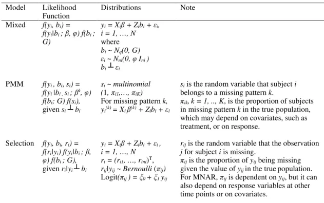
Table 2.2 presents the likelihood function of the joint distribution of yi and bi for
subject i. Upon integration over the random effects, the marginal distribution of yi is
Nni(Xiβ, ZiGZi>+φIni). When missing data exist inyi, the standard mixed-effects model
assumes that missing data are ignorable and the regression coefficients are estimated using
the observed data,yobs,i. Specifically, we can write
yobs,i =Xobs,iβ+Zobs,ibi+obs,i, i= 1, . . . , N,
whereXobs,i, Zobs,i, andobs,i are the subsets ofXi, Zi, andi, respectively, corresponding
Table 2.2: Examples of Mixed-effects Models, PMMs, and Selection Models
Model Likelihood Function
Distributions Note
Mixed f(yi, bi) =
f(yi|bi ; β, φ) f(bi ;
G)
yi = Xiβ + Zibi + εi,
i = 1, …, N
where
bi ~ Nq(0, G) εi ~ Nni(0, φ Ini )
bi┴εi
PMM f(yi, bi, si) =
f(yi|bi , si ; βk, φ)
f(bi; G) f(si), given si┴bi
si ~ multinomial
(1, πi1,…, πiK)
For missing pattern k, yi(k) = Xi β(k) + Zibi + εi
si is the random variable that subject i belongs to a missing pattern k.
πik,k = 1, .., K, is the proportion of subjects
in missing pattern k in the true population, which may depend on covariates, such as treatment, or on response.
Selection f(yi, bi,ri) =
f(ri|yi) f(yi|bi ; β, φ) f(bi ; G), given ri|yi ┴bi
yi = Xiβ + Zibi + εi ,
i = 1, …, N ri = (ri1, …, rini)T,
rij|yij ~ Bernoulli (πij) Logit(πij ) = ξ0 + ξ1 yij
rij is the random variable that the observation
j for subject i is missing.
πij is the proportion of yij being missing given the value of yij in the truepopulation. For MNAR, πij is dependent on yij, but it can also depend on response variables at other time points or on covariates.
2.3.2 Pattern-mixture Models
In addition to the response variables and the random effects, the likelihood function
of a PMM includes the missing pattern stratum variable si, which is usually assumed
independent of bi. For subject i, which is in pattern k, the likelihood function is given
by
Li,P M M =f(yi, bi, si) =f(si)f(yi|bi, si;βk, φ)f(bi;G),
where si ∼multinomial(1, πi1, . . . , πiK), and πi1, . . . , πiK are the proportion of subjects
in allK missing patterns in the true population, which may depend on covariates, such as
treatment, or on response. Moreover,yi, bi, andsi are assumed independent for different
subjects.
Conditional on the kth missing pattern, for subject i, the complete data yi = (ymis,i,
yobs,i) are given by
y(ik) =Xiβ(k)+Zibi+i,
where the superscript(k) onyi(k) indicates that subjectiis in missing pattern k, and β(k)
is ap×1 vector of unknown regression parameters specifically for patternk. Other model
assumptions are the same as those in the mixed-effects model. The PMM is conducted
by simply adding the covariate missing pattern and its interaction terms with other
fixed-effect covariates into a mixed-effect model. Parameter estimates can be obtained
by standard statistical software such as PROC MIXED in SAS.
The estimated response value given each dropout pattern can be obtained from
pattern-specific regression parameters. However, when estimating the response variable
for time points after dropout, additional assumptions (restriction) must be made, for
example, based on complete case, available case, or neighboring case (Fairclough, 2010).
These assumptions are not testable due to lack of data.
a weighted sum of pattern-specific estimates given by
E(y|X) =
K
X
k=1
E(y|X, pattern=k)πk,
where πk is the proportion of patients with the missing pattern, and X is fixed such as
treatment and baseline score.
A PMM assumes that a subject belongs to a specific missing pattern. When
perform-ing a PMM analysis, initially,K strata are created based on missing patterns. There are
several different ways of defining strata. In practice, the missing pattern strata are often
defined based on last visit before or after a certain time point (Hedeker and Gibbons,
1997). However, creating strata based only on last visit makes a strong assumption that
missing data within each stratum (i.e., intermittent missing) are ignorable (MCAR, or
MAR). Strata have also been defined based on reasons for withdrawal (e.g., death, disease
progression, toxicity, or other reason) (Pauler et al., 2003, Post et al., 2010). In
sum-mary, the choice of strata (or pattern) is a clinical judgment or is made for computational
convenience.
The parametersπik, k = 1, . . . , K, may or may not vary by subpopulation. In HRQOL
analysis, two popular assumptions are made on the mechanism, by which data are
miss-ing: (i) πik does not depend on any variable, or (ii) πik depends on treatment. Under
assumption (i), πik is estimated by the proportion of the kth missing pattern in the
whole sample. Under assumption (ii), πik is estimated by the proportion of the kth
missing pattern in each treatment group, separately.
2.3.3 Selection Models
Selection models get the name that observations were selected to be missing. Selection
models assume that the complete data, yi, follow a distribution and the probability of
probability of missingness, πij, may be assumed to follow a logistic regression in which
response may be included as a covariate. In selection models, the complete data yi =
(ymis,i, yobs,i) are typically assumed to follow the same model given by
yi =Xiβ+Zibi+i, i= 1, . . . , N.
The selection model introduces an ni vector of the missing data mechanism variable
ri = (ri1, . . . , ri,ni)
>, where r
ij = 1 indicating that yij is missing. Conditional on yi, ri is
commonly assumed to be independent ofbi. Thus, for subject i, the joint distribution of
yi, bi, and ri is given by
Li,SM =f(yi, bi, ri) =f(ri|yi)f(yi|bi;β, φ)f(bi;G),
where rij|yij ∼ Bernoulli(πij), and πij is the proportion of yij being missing given the
value of yij in the true population. f(ri|yi) is often modeled by logistic regression or
probit models. For MNAR, πij is dependent on yij, but it can also depend on response
variables at other time points or on covariates. For different subjects, yi, bi, and ri
are assumed independent. Ibrahim and Molenberghs (2009) and Ibrahim and colleagues
(2001) described the MCEM algorithm used for parametric estimation in selection models
(Ibrahim et al., 2001, Ibrahim and Molenberghs, 2009).
2.4 Simulation
We conducted an extensive simulation study to compare the three existing models
han-dling of missing data under various missing patterns and mechanisms.
2.4.1 Data Generation
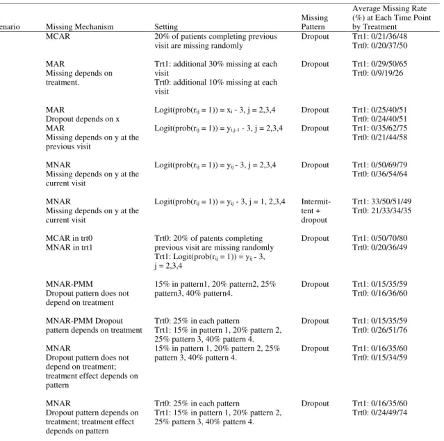
We simulated missing data on the response variable according to 10 different missing
(missing depending on treatment [scenario 2], the baseline score [scenario 3], or the
response at the previous assessment [scenario 4]); and MNAR (missing depending on
response at the current assessment [scenarios 5a and 5b]). We also considered intermittent
missing data in scenario 5b. Scenario 6 assumed that the missing mechanism was different
between two treatment groups: MCAR in one treatment group and MNAR in the other
treatment group. In scenarios 7 to 10, data were generated based on the assumption
of PMM. Specifically, subjects first were assigned randomly to one of the four dropout
groups: pattern 1, only one visit at time 1; pattern 2, last visit at time 2; pattern 3, last
visit at time 3; and pattern 4, last visit at time 4 (completer). In these scenarios, the
response variable depended on the dropout group to which a particular subject belonged.
In all scenarios, subjects were assigned randomly at a 1:1 ratio to one of the two treatment
groups. For each subject, a continuous baseline covariate xi was generated fromN(0,1),
and the random-effect variable bi was generated from N(0,1). The measurement errors
Table 2.3: Missing Data Mechanism and Missing Rate in Simulation Data
Scenario Missing Mechanism Setting
Missing Pattern
Average Missing Rate (%) at Each Time Point by Treatment
1 MCAR 20% of patients completing previous
visit are missing randomly
Dropout Trt1: 0/21/36/48
Trt0: 0/20/37/50
2 MAR
Missing depends on treatment.
Trt1: additional 30% missing at each visit
Trt0: additional 10% missing at each visit
Dropout Trt1: 0/29/50/65
Trt0: 0/9/19/26
3 MAR
Dropout depends on x
Logit(prob(rij = 1)) = xi - 3, j = 2,3,4 Dropout Trt1: 0/25/40/51
Trt0: 0/24/40/51
4 MAR
Missing depends on y at the previous visit
Logit(prob(rij = 1)) = yi,j-1 - 3, j = 2,3,4 Dropout Trt1: 0/35/62/75
Trt0: 0/21/44/58
5a MNAR
Missing depends on y at the current visit
Logit(prob(rij = 1)) = yij - 3, j = 2,3,4 Dropout Trt1: 0/50/69/79
Trt0: 0/36/54/64
5b MNAR
Missing depends on y at the current visit
Logit(prob(rij = 1)) = yij - 3, j = 1, 2,3,4
Intermit-tent + dropout
Trt1: 33/50/51/49 Trt0: 21/33/34/35
6 MCAR in trt0
MNAR in trt1
Trt0: 20% of patents completing previous visit are missing randomly Trt1: Logit(prob(rij = 1)) = yij - 3, j = 2,3,4
Dropout Trt1: 0/50/70/80
Trt0: 0/20/36/49
7 MNAR-PMM
Dropout pattern does not depend on treatment
15% in pattern1, 20% pattern2, 25% pattern3, 40% pattern4.
Dropout Trt1: 0/15/35/59
Trt0: 0/16/36/60
8 MNAR-PMM Dropout
pattern depends on treatment
Trt0: 25% in each pattern
Trt1: 15% in pattern 1, 20% pattern 2, 25% pattern 3, 40% pattern 4.
Dropout Trt1: 0/15/35/59
Trt0: 0/26/51/76
9 MNAR
Dropout pattern does not depend on treatment; treatment effect depends on pattern
15% in pattern 1, 20% pattern 2, 25% pattern 3, 40% pattern 4.
Dropout Trt1: 0/16/35/60
Trt0: 0/15/34/59
10 MNAR
Dropout pattern depends on treatment; treatment effect depends on pattern
Trt0: 25% in each pattern
Trt1: 15% in pattern 1, 20% pattern 2, 25% pattern 3, 40% pattern 4.
Dropout Trt1: 0/16/35/60
Trt0: 0/24/49/74
MAR = missing at random; MCAR = missing completely at random; MNAR = missing not at random; rij = indicator that yij is
The simulation data for scenarios 1 to 6 included 100 subjects with four planned
postbaseline visits. The response variables were generated using an equation given by
yij =β0+β1trti+β2xi+β3time2,ij +β4time3,ij+β5time4,ij+bi+ij,
where trti is the indicator for treatment (1 = trt 1, 0 = trt 0); xi is baseline score; and
time2,ij, time3,ij, andtime4,ij are indicator variables for visit time corresponding to times
2, 3, and 4 (time 1 is the reference level). By treating time as a categorical variable,
we allow the relationship between the response score and time to be nonlinear, which
is common in HRQOL data. We generated two sets of data–one with and one without
treatment effect. In the first set, we set the treatment parameter as 1. In the second set,
we set the treatment parameter as 0. In both sets, the parameters other than treatment
were set as 1, indicating that response score increased at the first two visits and then
remained stable after that.
For scenarios 7 through 10, a total of 200 subjects were randomly assigned to one of
the four dropout patterns: pattern 1, only one visit at time 1; pattern 2, last visit at
time 2; pattern 3, last visit at time 3; and pattern 4, last visit at time 4 (completer).
The proportion of each pattern was the same across treatments in scenarios 7 and 9 and
was treatment specific in scenarios 8 and 10. The response variables were generated by
yij = β0 +β1trti+β2xi+β3time2,ij+β4time3,ij+β5time4,ij
+ β6pattern1,i+β7pattern2,i+β8pattern3,i
+ β15time2,ij×trti +β16time3,ij×trti+β17time4,ij ×trti
+ β12time2,ij×pattern2,i+β13time2,ij ×pattern3,i+β14time3,ij ×pattern3,i
+ β9trti×pattern1,i+β10trti×pattern2,i+β11trti×pattern3,i
+ β18time2,ij×pattern2,i×trti+β19time2,ij ×pattern3,i×trti
where pattern1,i, pattern2,i, and pattern3,i were indicator variables for dropout pattern
corresponding to patterns 1, 2, and 3 (pattern 4, completer, is the reference group).
The pattern parameters were set as β6 = 3, β7 = 2, and β8 = 1, that is, patients in
the earlier dropout groups had higher (worse) response scores. The time-by-treatment
interaction parameters were set as β15 = 2, β16 = 1.5, and β17 = 1. The
pattern-by-time interactions involve only three, rather than nine, parameters (= 3×3) because,
except for the completer group (pattern 4), the responses after dropout could not be
observed or included in analysis. Therefore, there was no need to generate the value
of those responses in our simulation. For the same reason, the
treatment-by-time-by-pattern three-way interactions also involved only three parameters (β18, β19, β20). The
treatment effect in scenarios 9 and 10 depended on dropout pattern (β1 = 1, β9 =β10=
β11= 1, β18=β19=β20= 1), whereas in scenarios 7 and 8, the treatment effect did not
depend on dropout pattern (β1 = 1, β9 = β10 = β11 = 0, β18 = β19 =β20 = 0). We also
generated data with no treatment effect (β1 = 0, β9 =β10 = β11 = 0, β15 =β16 =β17 =
0, β18=β19=β20= 0). In all scenarios, we set β2 =β3 =β4 =β5 = 1.
Data were generated using SAS for Windows (Version 9.2). Table 2.3 summarizes the
average missing rate from the simulated data by treatment group and time point. For
example, in scenario 1, there were no missing data at time 1, and the missing rate at
time 2 was 21% among the trt 1 group and 20% among the trt 0 group.
2.4.2 Analysis of the Simulated Data
For each simulation scenario, three models, including a mixed-effects model, a PMM,
and a selection model, described as follows were fitted to estimate the treatment effect.
Analysis for scenarios 1 to 6 (treatment effect does not vary by time)
For the mixed-effects model, the analysis included all observed visits. The models
Specifically, we specified
yij =β0+β1trti+β2xi+β3time2,ij +β4time3,ij+β5time4,ij+bi+ij.
The treatment effect was estimated byβ1. Parameter estimates and the estimates of the
standard error were obtained using PROC MIXED (SAS for Windows, Version 9.2).
For the PMM analysis, subjects in the simulated data first were grouped into four
dropout patterns based on the last visit. The sample proportion of the dropout groups
was calculated for the overall sample and for each treatment group separately. The
proportion was calculated using the number of subjects in each pattern group divided by
the total number of subjects. The analysis models included fixed effects and the random
intercept, as follows:
yij = β0+β1trti+β2xi+β3time2,ij+β4time3,ij+β5time4,ij
+ β6pattern1,i+β7pattern2,i+β8pattern3,i
+ β9trti ×pattern1,i+β10trti×pattern2,i+β11trti×pattern3,i
+ bi+ij.
The parameters were estimated using PROC MIXED based on all observed visits.
Then, using the model described previously, two estimates of the overall treatment effect
were obtained, one using the overall proportion of the dropout pattern and the other
using the treatment-specific proportion of the dropout pattern. The variance of the
treatment effects was obtained using the delta methods (Pauler et al., 2003).
The selection model contained the same fixed and random effects as the mixed model.
In addition, the probability of missingness was modeled by using logistic regression with
the current response variable as the covariate. For dropout missingness, only the first
Therefore, the missing data after the first missing were not included in the logistic
re-gression. Analysis was performed using R software.
Analysis for scenarios 7 to 10 (treatment effect varied by time)
In this set of scenarios, we allowed treatment effect to vary by time by adding treatment
by time interaction. For the mixed-effects model and selection model analyses, we added
the time-by-treatment interactions (3 terms: time2×trt;time3×trt;time4×trt) as fixed
covariates. The treatment effects were estimated for each time point.
For PMM, to obtain pattern-specific estimates, the model was specified in the same
way as data were generated. Note that only three time-by-pattern interaction terms and,
correspondingly, three time-by-pattern-by-treatment interaction terms were included in
the model. Other time-by-pattern and time-by-pattern-by-treatment interactions were
not estimable because of the missing pattern. The estimates of overall treatment effect
were obtained using the overall proportion of dropout pattern and the treatment-specific
proportion of dropout pattern as described previously.
2.5 Results
For scenarios 1 to 6, which do not include time-by-treatment interaction effect, Table
2.4 presents the simulation results for the estimates from the mixed-effects model, PMM,
and selection model. One estimate from the PMM was based on the overall proportion of
dropout groups, and the other was based on the treatment-specific proportion of dropout
groups.
Although the PMM and the selection model were designed to handle MNAR data,
both provided unbiased estimates of treatment effect (0.96 to 1.01) when missingness
did not depend on response. This was the case for scenario 1, in which, at each time
point, 20% of subjects completing previous visit were missing randomly; scenario 2, in
the probability of missingness response depended on the baseline score. As expected,
the mixed-effects model also provided unbiased estimates of treatment effect in these
scenarios.
When missingness depended on the observed response at the previous time point
(sce-nario 4) but not the current time point, the mixed-effects model provided an unbiased
estimate (1.03) as expected. However, the estimates from the PMM were biased,
espe-cially when the PMM estimates were based on the overall proportion of dropout groups.
The estimate from the selection model was also biased. This suggested that the selection
model might be sensitive to the parametric form of the missing mechanism, which was
not testable from the data.
When missingness at a visit depended on the current response (scenarios 5a and 5b),
the selection model built on such a missing mechanism provided an unbiased estimate.
Estimates of treatment from both the mixed-effects model and PMM were biased. This
was observed when the missing data were related to dropout or were intermittent. The
magnitude of the bias was the smallest for the PMM based on treatment-specific
propor-tion when missing data contained only dropout and was the largest for the PMM using
the overall proportion of dropout groups.
In scenario 6, the missing mechanism was different between treatment groups; 20%
of data were randomly missing among those who completed the previous visit in one
treatment group, while the missingness depended on the current response in the other
treatment group. In this scenario, the estimates from the selection model and the
esti-mates from the PMM based on the treatment-specific proportion were better than those
Table 2.4: Average Treatment Effect and Its Standard Error Estimated from the Mixed-Effects Model, the Pattern-Mixture Model, and the Selection Model for Scenarios 1 to 6 (true treatment effect = 1)
(a) Point estimate of treatment effect
Scenario Mixed PMM (ova) PMM (trb) Selection Model
1 MCAR 1.00 1.00 1.01 1.00
2 MAR (trt) 0.96 0.96 0.96 1.00
3 MAR (x) 0.99 1.00 0.99 0.98
4 MAR (yt-1) 1.03 0.73c 1.08c 1.07c
5a MNAR (yt) 0.92c 0.77c 0.94c 0.97
5b MNAR (yt) Intermittent missing 0.79c 0.71c 0.79c 0.99
6 MCAR in trt0, MNAR(yt) in trt1 0.80c 0.73c 0.90c 0.91c
(b) Standard error
Mixed PMM (ov)a PMM (tr)b Selection Model
Scenario Emp.
SE SE est.
Emp.
SE SE est.
Emp.
SE SE est.
Emp.
SE SE est.
1 MCAR 0.24 0.24 0.23 0.25c 0.24 0.25c 0.22 0.24c
2 MAR (trt) 0.27 0.24c 0.30 0.28c 0.26 0.25c 0.26 0.24c
3 MAR (x) 0.24 0.24c 0.25 0.26c 0.25 0.26c 0.21 0.24c
4 MAR (yt-1) 0.25 0.24c 0.22 0.22 0.27 0.27 0.21 0.27c
5a MNAR (yt) 0.24 0.24 0.25 0.24c 0.25 0.26c 0.23 0.25c
5b MNAR (yt) Intermittent missing 0.22 0.22c 0.21 0.23c 0.22 0.23c 0.20 0.23c
6 MCAR in trt0, MNAR(yt) in trt1 0.22 0.25c 0.26 0.28c 0.23 0.26c 0.21 0.24c
Emp = Empirical; est = estimate; MCAR = missing completely at random; MAR = missing at random; MNAR = missing not at random; PMM pattern-mixture model; SE = standard error; trt = treatment.
a Treatment effects estimated using proportion of dropout in overall sample (ov).
b Treatment effects estimated using treatment-specific proportion of dropout (tr).
c The 95% confidence interval does not cover the true value.
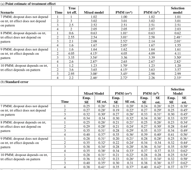
Table 2.5: Average Treatment Effect and Its Standard Error Estimated from the Mixed-Effects Model, the Pattern-Mixture Model, and the Selection model for Scenarios 7 to 10
(a)Point estimate of treatment effect
Scenario Time
True
trteff. Mixed model PMM (ova) PMM (trb)
Selection model 7 PMM; dropout does not depend
on trt, trt effect does not depend on pattern
1 1 1.02 1.00 1.02 1.01
2 3 3.02 3.01 3.02 3.01
3 2.5 2.52 2.51 2.51 2.51
4 2 2.05 2.05 2.07 2.03
8 PMM; dropout depends on trt, trt effect does not depend on pattern
1 0.6 0.63 1.01c 0.63 0.62
2 2.55 2.54 3.01c 2.58 2.48 c
3 2.1 2.08 2.52c 2.14 2.01c
4 1.6 1.67 2.05c 1.67 1.55
9 PMM; dropout does not depend on trt, trt effect depends on pattern
1 1.6 1.64 1.62 1.64 1.61
2 4.05 4.15c 4.05 4.09 4.11
3 3.35 3.54c 3.36 3.39 3.50c
4 2.6 2.87c 2.65 2.67 2.82c
10 PMM; dropout depends on trt, trt effect depends on pattern
1 1.2 1.23 1.70c 1.23 1.20
2 3.6 3.65 4.15c 3.63 3.57
3 2.95 3.08c 3.45c 2.98 2.99
4 2.2 2.46c 2.72c 2.26 2.33c
(b)Standard error
Mixed Model PMM (ova) PMM (trb)
Selection Model
Time
Emp.
SE SE est.
Emp.
SE SE est.
Emp. SE
SE est.
Emp. SE
SE est. 7 PMM; dropout does not depend
on trt, trt effect does not depend on pattern
1 0.25 0.26c 0.21 0.20c 0.24 0.26c 0.25 0.38c
2 0.27 0.28c 0.19 0.22c 0.27 0.29c 0.25 0.45c
3 0.32 0.30c 0.27 0.26c 0.33 0.31c 0.30 0.45c
4 0.34 0.34 0.30 0.32c 0.34 0.36c 0.33 0.55c
8 PMM; dropout depends on trt, trt effect does not depend on pattern
1 0.25 0.26c 0.21 0.21c 0.25 0.26c 0.23 0.34c
2 0.29 0.28c 0.21 0.24c 0.27 0.30c 0.28 0.44c
3 0.35 0.31c 0.28 0.29c 0.35 0.33c 0.34 0.49c
4 0.40 0.37c 0.35 0.36c 0.39 0.40c 0.41 0.56c
9 PMM; dropout does not depend on trt, trt effect depends on pattern
1 0.28 0.31c 0.20 0.21c 0.28 0.28c 0.25 0.36 c
2 0.35 0.32c 0.22 0.24c 0.34 0.34 0.32 0.44c
3 0.38 0.34c 0.28 0.28c 0.36 0.34c 0.35 0.50c
4 0.35 0.38c 0.34 0.33c 0.37 0.37 0.33 0.62c
10 PMM; dropout depends on trt, trt effect depends on pattern
1 0.28 0.31c 0.21 0.22c 0.28 0.28 0.25 0.54c
2 0.36 0.32c 0.23 0.26c 0.33 0.34c 0.32 0.58c
3 0.40 0.35c 0.30 0.31 0.38 0.36c 0.37 0.62c
4 0.38 0.41c 0.35 0.37c 0.40 0.42c 0.37 0.77c
Emp = Empirical; est = estimate; PMM = pattern-mixture model; SE = standard error; trt = treatment.
a Treatment effects estimated using proportion of dropout in overall sample (ov).
b Treatment effects estimated using treatment-specific proportion of dropout (tr).
c The 95% confidence interval does not cover the true value.
For scenarios 7 to 10, data were generated from the preidentified dropout patterns,
and the treatment effects varied by time; therefore, the treatment effects were estimated
at each time point. Table 2.5 presents the simulation results. The PMM estimates based
on the treatment-specific proportion were unbiased in all four scenarios as expected.
The PMM estimates using overall proportion were unbiased when the dropout
distri-bution did not depend on treatment (scenarios 7 and 9), but they were biased when the
dropout distribution depended on treatment (scenarios 8 and 10). When the dropout
distribution did not depend on treatment, the estimates based on overall proportion were
more efficient (smaller standard error [SE]) than those based on the treatment-specific
proportion. When the treatment effects depended on the dropout pattern (scenarios 9
and 10), estimates obtained from the mixed-effects model was biased at later time points.
However, the mixed-effects model provided unbiased estimates of treatment effect in the
scenarios in which treatment effect did not depend on dropout pattern (scenarios 7 and
8), even though the response depended on dropout pattern. The selection model
pro-vided biased results at some time points, when either dropout depended on treatment or
treatment effect depended on dropout pattern, although the magnitude of bias was small
(<10%). Tables 2.4(b) and 2.5(b) present the simulation results on SE estimates. Except
for a few cases, the SEs from the mixed-effects model, the PMM, and the selection model
are all biased (the 95% confidence interval does not cover the true value.)
When there was no true treatment effect (i.e., parameters for treatment were 0), the
bias was less than 0.10 for all models, except for scenario 6, in which treatments had
different missing mechanisms. In scenario 6, the bias from PMM estimates using overall
proportion (-0.16) was larger than that from the mixed model (-0.12), selection model
2.6 Conclusions
Our simulation results suggest that the treatment effect defined as difference in expected
value of the response variable given the same baseline was unbiased when the model
assumption on missing mechanism holds. Pattern-mixture model provides good estimates
when subjects are from different missing patterns. The selection model provides good
estimates when the probability of missingness is dependent on the value of response
variable. When the model assumption does not hold, the estimate is biased. There is
not a model that consistently performs better than others. However, the PMM using
the treatment-specific proportion and the selection model provide some correction of the
estimate compared with the mixed-effects model in several MNAR situations, even when
the mechanism of missing data is not exactly the same as the model assumption.
To obtain the overall treatment effect from the PMM, the treatment-specific
pro-portion of missing pattern should be used in most cases. The overall treatment effect
obtained based on the overall proportion of the pattern should be used only when the
dropout proportion does not depend on treatment. In this situation, the estimate is
equivalent to the estimate based on the treatment-specific proportion but is more
effi-cient.
For selection models, when the probability of missingness depends on the previous
response, the estimates from the selection model used in analysis, which specify that the
probability of missingness depends on current response in the logit model, are biased.
However, this will be improved if the logit model includes the previous response as a