PRACTICAL PHOTON MAPPING IN HARDWARE
Joshua Eli Steinhurst
A dissertation submitted to the faculty of the University of North Carolina at Chapel Hill in partial fulfillment of the requirements for the degree of Doctor of Philosophy in the Department of Computer Science.
Chapel Hill 2007
Approved by:
Dr. Anselmo Lastra
Dr. Gary Bishop
Dr. Leonard McMillian
Dr. Steven Molnar
c
2007
ABSTRACT
JOSHUA ELI STEINHURST: Practical Photon Mapping in Hardware (Under the direction of Dr. Anselmo Lastra)
Photon mapping is a popular global illumination algorithm that can reproduce a wide range of visual effects including indirect illumination, color bleeding and caustics on com-plex diffuse, glossy, and specular surfaces modeled using arbitrary geometric primitives. However, the large amount of computation and tremendous amount of memory band-width, terabytes per second, required makes photon mapping prohibitively expensive for interactive applications.
In this dissertation I present three techniques that work together to reduce the band-width requirements of photon mapping by over an order of magnitude. These are com-bined in a hardware architecture that can provide interactive performance on moderately-sized indirectly-illuminated scenes using a pre-computed photon map.
1. The computations of the naive photon map algorithm are efficiently reordered, generating exactly the same image, but with an order of magnitude less bandwidth due to an easily cacheable sequence of memory accesses.
2. The irradiance caching algorithm is modified to allow fine-grain parallel execution by removing the sequential dependency between pixels. The bandwidth require-ments of scenes with diffuse surfaces and low geometric complexity is reduced by an additional 40% or more.
Combined Importance Sampling is simple to implement, cheap to compute, com-patible with query reordering, and can reduce bandwidth requirements by an order of magnitude.
ACKNOWLEDGMENTS
This dissertation, and the research that it documents, could never have been accomplished without the selfless assistance of others. Intellectually, I am indebted to all my instructors, classmates and colleagues who have together prepared me for this task. Since arriving in Chapel Hill, Dr. Anselmo Lastra has been my advisor, guiding me with patience and understanding through the process of finding and pursuing my topic to completion. I have learned a lot from him about the conduct and presentation of research. Additionally, I have received more grammar lessons “then” shall be mentioned here.
My committee, Dr. Gary Bishop, Dr. Leonard McMillan, Dr. Steven Molnar and Dr. Jan Prins, have provided me with thoughtful suggestions at every step and have graciously accommodated changes to my timeline. Much of the direct inspiration for this research arose from the discussions and work of the Advanced Research in Graphics Hardware (ARGH!) group. In particular, Justin Hensley and Greg Coombe have served as co-authors, collaborators and informed sounding boards throughout the entire process. During my stay in Chapel Hill the talented computer science department staff pro-vided a pleasurable and productive working environment. This is also true of ITS who supported the computational research cluster on which the dissertation experiments were executed.
Enjoying food and shelter as I do, I am grateful to the funding sources that have permitted me to do this research: the state of North Carolina, the National Science Foundation, the NVIDIA Corporation, and the Paul Hardin Dissertation Fellowship.
transformed my rough diagrams into polished images worthy of publication, and Thorsten Scheuermann, who assisted with editing.
Throughout my life I have been supported, encouraged, and taught by my parents, family, and friends. Without their backing I would not be the person that I am, and this dissertation would certainly not have been attempted, much less completed. Mom, Dad, Dan, Sarah, Ben, Bubbie, Zayde, the rest of my wonderful family, my life long friends from Montpelier, my college and graduate school friends: you have kept my spirits hight and priorities straight. Thank you.
TABLE OF CONTENTS
LIST OF TABLES xiii
LIST OF FIGURES xiv
LIST OF ALGORITHMS xvii
1 Introduction 1
1.1 Realistic image synthesis . . . 2
1.2 Photon mapping . . . 4
1.3 Summary of original contributions . . . 5
1.4 Scenes of interest . . . 7
1.5 Dissertation summary . . . 9
2 Background 11 2.1 The evolution of graphics hardware . . . 11
2.2 Target implementation technology . . . 14
2.3 Realistic image synthesis . . . 16
2.3.1 Radiometry . . . 17
2.3.2 The rendering equation . . . 20
2.3.3 Numerical integration . . . 25
2.3.4 Monte Carlo integration . . . 26
2.4 Global Illumination algorithms . . . 27
2.4.1 Path tracing . . . 28
2.4.1.2 Stochastic ray tracing . . . 29
2.4.1.3 Additional path tracing algorithms . . . 31
2.4.2 Radiosity . . . 32
2.4.3 Discussion . . . 32
2.5 Fifth generation graphics architectures . . . 33
2.6 Photon mapping . . . 34
2.6.1 Photon map creation . . . 35
2.6.2 Image generation . . . 37
2.6.2.1 Final gather visualization . . . 39
2.6.3 Computational Requirements . . . 40
2.6.4 Bandwidth Requirements . . . 41
2.7 Discussion . . . 41
3 Photon Gather Reordering 43 3.1 Origin of the high costs . . . 44
3.2 Reordering algorithms . . . 46
3.3 Generative reordering . . . 47
3.3.1 Tiled reordering . . . 48
3.3.2 Tiled direction-binning reordering . . . 49
3.4 Deferred reordering . . . 52
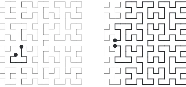
3.4.1 Hilbert curve reordering . . . 52
3.4.2 Tiled Hilbert reordering . . . 54
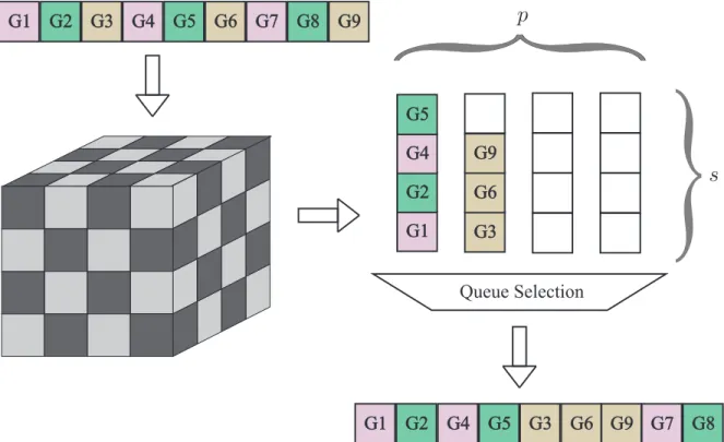
3.4.3 Hashed reordering . . . 55
3.4.4 Tiled direction-binning Hashed reordering . . . 57
3.5 Cache parameters . . . 58
4 Data Structures 61
4.1 Uniform grid . . . 62
4.2 kd-tree . . . 63
4.3 kdB-tree . . . 65
4.4 Block Hashing . . . 66
4.5 Conclusion . . . 67
5 Irradiance Caching 70 5.1 The Irradiance Cache . . . 71
5.1.1 Error Estimate . . . 73
5.1.2 The Algorithm . . . 75
5.1.3 Discussion . . . 76
5.2 Tiled irradiance caching . . . 80
5.3 Pre-computing the harmonic mean distance . . . 82
5.4 Interaction with photon gather reordering . . . 84
5.5 Possible Extensions . . . 86
5.6 Conclusions . . . 88
6 Importance Sampling 90 6.1 Background . . . 91
6.1.1 Importance sampling . . . 94
6.1.2 Multiple importance sampling . . . 98
6.2 Sampling the rendering equation . . . 99
6.2.1 Sampling the BRDF . . . 101
6.2.2 Sampling the incident radiance function . . . 102
6.2.3 Jensen’s method . . . 103
6.2.3.1 Resource requirements . . . 107
6.2.4.1 Resource requirements . . . 109
6.2.5 Pharr’s method . . . 110
6.2.5.1 Resource requirements . . . 111
6.3 Combined importance sampling . . . 111
6.3.0.2 Resource requirements . . . 115
6.3.0.3 Discussion . . . 115
6.4 Results . . . 115
6.4.1 Comparison of variance . . . 116
6.4.2 Generated image quality . . . 119
6.5 Interaction with gather reordering . . . 122
6.6 Conclusion . . . 124
7 Architecture 125 7.1 Goals and constraints . . . 126
7.2 System overview . . . 129
7.2.1 Duties of the host . . . 130
7.2.2 Interconnect bandwidth . . . 131
7.3 The rendering chip . . . 131
7.3.1 The rendering of a tile . . . 133
7.3.2 Ray casting unit . . . 135
7.3.2.1 Computation . . . 138
7.3.2.2 Memory bandwidth . . . 139
7.3.2.3 Storage . . . 139
7.3.3 Controller . . . 139
7.3.3.1 Computation . . . 142
7.3.3.2 Storage . . . 143
7.3.4.1 Computation . . . 147
7.3.4.2 Storage . . . 148
7.3.4.3 External bandwidth . . . 148
7.3.5 Summary of costs . . . 149
7.4 Simulation and analysis . . . 151
7.4.1 Test scenes . . . 152
7.4.2 Single chip performance . . . 156
7.4.3 Expected system performance . . . 158
7.5 Discussion . . . 158
7.5.1 Load Balancing . . . 159
7.5.2 Scalability . . . 159
7.5.3 Progress and deadlock . . . 160
7.5.4 Limitations . . . 162
8 Summary and Conclusion 164 8.1 Research Contributions . . . 164
8.2 Limitations . . . 167
8.3 Future Work . . . 168
8.4 Conclusion . . . 171
LIST OF TABLES
2.1 Radiometric symbols, terms, and units . . . 18
3.1 Summary of reordering performance . . . 60
4.1 Cache block fetches for various reorderings and data structures . . . 67
5.1 Interaction between irradiance caching and query reordering . . . 85
5.2 Summary of irradiance performance . . . 88
6.1 Importance sampling storage cost comparison . . . 114
6.2 Importance sampling computation cost comparison . . . 116
7.1 Cost analysis notation . . . 129
7.2 Packet composition: Ray caster to controller . . . 136
7.3 Packet composition: Ray caster to photon gatherer . . . 138
7.4 Packet composition: Controller to photon gatherer . . . 140
7.5 Packet composition: Controller to ray caster . . . 141
7.6 Packet composition: Photon gatherer to controller . . . 147
7.7 Summary of computational costs for a single tile . . . 149
7.8 Summary of inter-unit bandwidth costs for a single tile . . . 150
7.9 Summary of on-chip storage requirements . . . 151
7.10 Single chip performance . . . 157
LIST OF FIGURES
1.1 Visual effects supported by Photon Mapping . . . 4
1.2 The modified Cornell box . . . 8
1.3 The Sponza atrium . . . 9
2.1 Growth in GPU computation . . . 15
2.2 Growth in GPU bandwidth . . . 16
2.3 Radiance . . . 19
2.4 The invariance of radiance . . . 20
2.5 Image formation with an ideal pinhole camera . . . 21
2.6 Examples of common BRDF classifications . . . 24
2.7 Computing reflected radiance using a photon gather . . . 39
2.8 Final gather visualization of the photon map . . . 40
3.1 Coherence between successive photon gathers . . . 44
3.2 Overview of reordering . . . 46
3.3 Eye-ray coherence of image tiles . . . 48
3.4 Tiled direction-binning reordering . . . 49
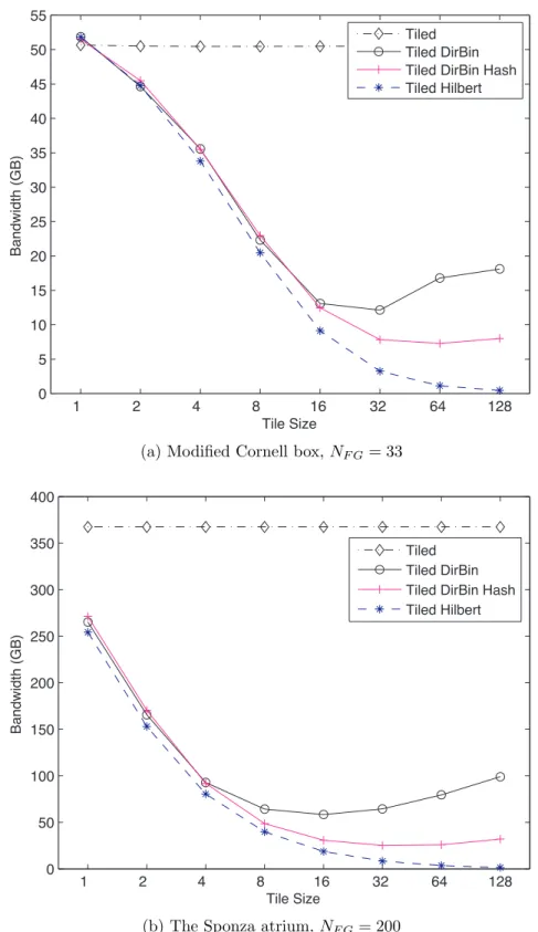
3.5 Reordering bandwidths for varying tile sizes . . . 51
3.6 The Hilbert curve . . . 53
3.8 Hashed reordering . . . 56
3.9 Bandwidths for various cache sizes . . . 59
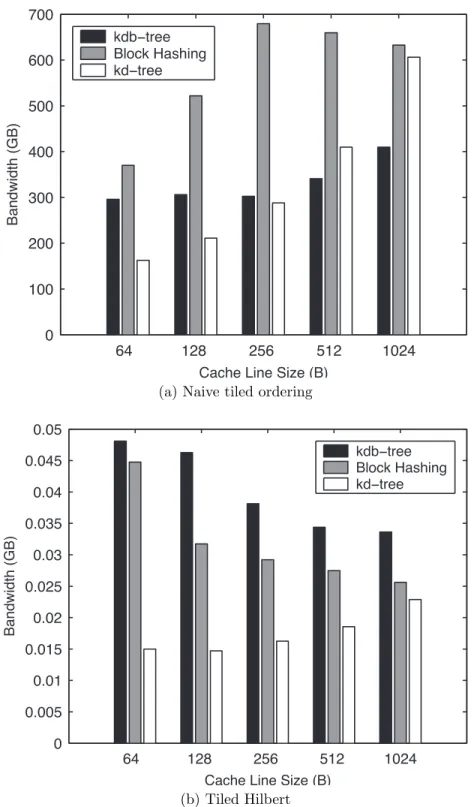
4.1 Interaction between cache line size and bandwidth for various data structures 68 5.1 The commonly low spatial variance of indirect illumination . . . 71
5.2 The split-sphere model . . . 74
5.3 Varying max for the Cornell box . . . 77
5.4 Varying max for the Sponza atrium . . . 78
5.5 Complex geometry reducesRIC . . . 79
5.6 Tiled irradiance caching . . . 81
5.7 Pre-computing Ravg at a subset of photons . . . 83
5.8 Reordering bandwidths for varying tile sizes with irradiance caching . . . 87
6.1 Example g(x) . . . 92
6.2 Blind Monte Carlo integration . . . 93
6.3 ChoosingXi according top(x) . . . 95
6.4 Computing g(cp−1(x()x)) . . . 96
6.5 Importance sampling g(x) . . . 97
6.6 Importance sampling a more uniform function . . . 97
6.7 The beach lightprobe example . . . 100
6.9 Jensen’s importance sampling . . . 104
6.10 Importance sampling with Hey’s method . . . 108
6.11 Graphical representation of combined importance sampling . . . 114
6.12 Importance sampling convergence for two lightprobes . . . 118
6.13 Visual and graphical variance in the dome scene . . . 120
6.14 System tradeoffs with combined importance sampling . . . 121
6.15 Importance sampling of an acquired BRDF . . . 121
6.16 Interaction between reordering and importance sampling . . . 122
6.17 Interaction between reordering and importance sampling . . . 123
7.1 Overall system diagram . . . 130
7.2 Rendering chip diagram . . . 132
7.3 Photon gatherer . . . 145
7.4 Two variations of the Cornell box . . . 154
7.5 Two variations of a box with a glossy floor . . . 155
LIST OF ALGORITHMS
2.1 The pixel-driven rendering algorithm . . . 22
2.2 Whitted-style ray tracing . . . 29
2.3 Stochastic ray tracing . . . 30
2.4 Photon map creation . . . 36
2.5 Generation of an image using the photon map . . . 38
6.1 Preprocessing for Jensen’s method . . . 105
6.2 Generating samples with Jensen’s method . . . 106
CHAPTER 1 INTRODUCTION
“Computer graphics is now a mature discipline. Both hardware and software are available that facilitate the production of graphical images as diverse as line drawings and realistic renderings of natural objects. A decade ago the hardware and software to generate these graphical images cost hundreds of thousands of dollars. Today, excellent facilities are available for expenditures in the tens of thousands of dollars . . . ”
— Procedural Elements For Computer Graphics (Rogers, 1985, xi)
Not only has the cost of graphics hardware fallen by an order of magnitude each of the last three decades, but the expectations of graphics consumers has grown correspondingly. The original applications that inspired and funded early computer graphics research, such as scientific visualization, Computer Aided Design (CAD), and flight simulators, continue to flourish. However, the primary driver of the computer graphics industry, and therefore research, is now entertainment applications such as movies and video games, which have insatiable demands for higher quality imagery.
In 2005, domestic video game sales overtook movie box office receipts (Crandall and Sidak, 2006; MPAA, 2006). Much of this success can be attributed to the increas-ing sophistication of consumer graphics hardware available at reasonable prices. This has allowed game developers to produce interactive experiences that are visually closer to movies. There is a crucial difference that explains the still obvious gap in quality. Movies require the generation of approximately one quarter of a million images, but only once. Stored on film or disk, the images are simply displayed to viewers. Interactive video games, however, must produce dozens of unique images every second for each and every player. Even with the most powerful commodity graphics hardware available, only a simplistic light transport algorithm can typically be used. This dissertation presents a novel architecture that can interactively generate images using an advanced light trans-port algorithm, photon mapping. This will allow for more photo-realistic imagery in interactive applications such as video games.
1.1
Realistic image synthesis
Modelling the interaction of light and the objects in a scene is the essence of realistic image synthesis. The detail with which we can specify the geometry of a scene has improved remarkable over the years. Commodity graphics hardware allows the interactive viewing of all but the largest of scenes. It is the more accurate simulation of light transport that will differentiate the next generation of graphics hardware.
Real world illumination at a single point, however, is dependent on the entire scene. One object may cast a shadow on another, light may bounce indirectly off of multiple objects, there may be highly specular mirrors, caustics may form, etc. These effects can be painstakingly added one by one to an image generated with local illumination models using single purpose rendering algorithms such as shadow volumes (Heidmann, 1991), environment maps (Blinn and Newell, 1976; Greene, 1986), pre-computed radiosity tex-tures (Cohen and Wallace, 1993), or even a highly specific glittering gem effect (Gosselin, 2004).
However, these algorithms are hard to combine or generalize and often fail to capture essential parts of the underlying physics: the shadow maps may cause aliasing; environ-ment maps are generally incorrect; the sparkling gem effect may fail when the gem is submerged in water; and the pre-computed radiosity textures have to be recomputed if the scene changes significantly. A more accurate simulation will require less programmer and artist time for each scene. It will therefore be more economical as processing power becomes more plentiful and cheap relative to the salaries of skilled labour. Generic global illumination models, used at least partially in many photo-realistic renderings, create the visual effects directly by simulating, with varying accuracy, the physics of light transport between objects in a scene.
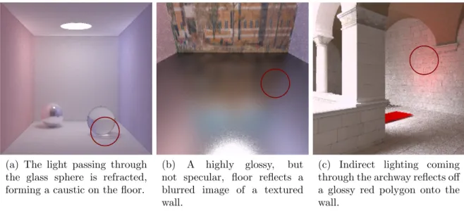
(a) The light passing through the glass sphere is refracted, forming a caustic on the floor.
(b) A highly glossy, but not specular, floor reflects a blurred image of a textured wall.
(c) Indirect lighting coming through the archway reflects off a glossy red polygon onto the wall.
Figure 1.1: Photon mapping is a powerful and efficient global illumination algorithm. These images demonstrate some particular effects handled well by photon mapping. This dissertation presents a hardware architecture capable of rendering these images at inter-active rates.
1.2
Photon mapping
Photon mapping (Jensen, 1996a; Jensen, 2001) is a popular and robust global illumi-nation algorithm. It can reproduce a wide range of visual effects including indirect illumination, color bleeding, and caustics on complex diffuse, glossy and specular sur-faces represented using arbitrary geometric primitives, as demonstrated in Figure 1.1. The algorithm generates an image in two phases.
The first phases breaks the energy of the light sources into discrete packets called photons1. The photons are shot into space and allowed to probabilistically reflect, refract
and be absorbed by surfaces. At every intersection with the scene, the photons, their locations, energy, and direction of travel, are recorded in the photon map.
The actual image is generated in the second phase. Although the process has multiple steps (see Chapter 2 for details) it uses the photon map as an estimate of the amount
1The term photon is somewhat misleading because they do not represent actual physical photons.
and quality of light arriving at any point in the scene from all directions. To estimate the incident radiance, a photon gather is performed. This is essentially a k -Nearest-Neighbors (kNN) search, finding the k photons closest to the point of interest from the map. The photon gather is used to terminate, at an early stage, the recursive evaluation of light transport.
The realism of the photon mapping comes at a cost, in terms of both computation and memory bandwidth. Using the naive photon map algorithm on the Sponza scene, as described in Section 1.4 and shown in Figure 1.3, 145 million floating point operations are required for a single 512×512 image. This computational cost is significant, but manageable given the tremendous increase in semiconductor capabilities. The memory bandwidth requirements, 367 Gigabytes (GB) per image, is a more significant problem because off-chip bandwidth has not improved at the same rate as computational power. This cost is very significant for interactive applications that must generate a new image dozens of times a second. At thirty images a second, the memory bandwidth requirement reaches 11 Terabytes (TB) per second. In current semiconductor technology this is a prohibitively large bandwidth for a desktop-sized machine. Improvements are therefore necessary if photon mapping is to be made practical for interactive use.
1.3
Summary of original contributions
This dissertation presents several novel techniques to dramatically reduce the bandwidth cost of photon mapping. These techniques are then combined into a practical hardware architecture that can support interactive applications. Taken together, these contribu-tions support my thesis statement:
Specifically, the architecture combines the following techniques to reduce the bandwidth requirements of photon mapping:
Low bandwidth photon gathers using reordering: Photon-gather reordering pro-duces the same image as the naive photon mapping algorithm, but reorders the computations such that the memory accesses are more coherent (Steinhurst et al., 2005). A 128 KB cache is then able to exploit this coherence and reduce the band-width to main memory by over an order of magnitude.
Tiled irradiance caching with pre-computed radius for split-sphere heuristic: Irradiance caching is commonly used to reduce the number of final gathers re-quired (Ward et al., 1988). However, the conventional irradiance caching algorithm creates a sequential dependency between the pixels of an image preventing either efficient parallel execution or the application of photon-gather reordering. The image is divided into tiles each with a separate irradiance cache. To remove the dependency within each tile, I present a new technique for calculating the split-sphere heuristic. Together these technqiues provide a means to apply irradiance caching to a finely-grained parallel photon mapper without introducing significant additional error to the generated images.
1.4
Scenes of interest
The intended use of the photon mapping architecture is for interactive applications such as video games and architectural walkthroughs. To evaluate the proposed system I have used variations on two scenes with the following qualities:
• Varied surface reflectance properties: diffuse, glossy and specular. This is important
to fully test the combined importance sampler. It also allows a more complete evaluation of gather reordering when considerable coherence is already present in the gather requests.
• A camera position that views less than half of the scene. This exposes a potential
weakness of bi-directional global illumination algorithms such as photon mapping, in that effort may be wasted because not all of the photon map is used.
• Varied illumination complexity. The light in scenes with high illumination
complex-ity must navigate through several reflections before entering the camera. In scenes such as these, the indirect illumination is very important and is a good case for photon mapping. In simpler scenes most of the light is due to direct illumination and the indirect illumination calculated by photon mapping is subtle.
These requirements will result in a fair evaluation of photon mapping, irradiance caching, importance sampling, and query reordering, thereby making the architecture simulation representative of the desired workload. I have chosen two basic scenes that, with some variations, meet these criteria and sample the space of potential uses:
Figure 1.2: Several variations of this global illumination test scene, a slightly modified Cornell box, are used in this dissertation. Note that the scene is a simple box with a single area light, a mirrored sphere and a glass sphere, and colored walls. This scene exhibits indirect illumination as color bleeding, reflections, and a bright focused caustic under the glass sphere. This image using the naive photon mapping algorithm requires 50 gigabytes of memory bandwidth and 37 billion floating point operations.
a variation of the standard Cornell box, Figure 1.2, traditionally used for global il-lumination evaluation. The geometry is very simple, a handful of rectangles, but it meets the other criteria. In later chapters I will use further variations, for example adding extra objects for complexity or changing the surface reflectance. Alterna-tively, the light may be replaced by a spot light aimed at the ceiling, eliminating any direct lighting, thus emphasizing the requirements for a quality computation of the indirect illumination.
Figure 1.3: The Sponza atrium, modeled by Marko Dabrovic of RNA Studios and used with permission, is a large complex structure with a central atrium and corridors that overlook the atrium. The sky is modeled as an area light the size of the top opening, all illumination in the corridors is indirect. The naive photon mapping algorithm generates 367 gigabytes of traffic to the photon map memory and uses 209 billion floating point operations.
geometry is complicated and is composed of different regions with small openings onto a shared atrium. The light is modeled as coming from the sky, a large area light. The light spilling through the archway is all indirect. Without global illumi-nation this scene would be mostly black. Minor variations such as the introduction of small glossy reflectors are used in evaluating the architecture.
1.5
Dissertation summary
This dissertation is divided into three parts: background, individual techniques, and the combined architecture. Chapter 2 provides an overview of the evolution of graphic hardware architectures, global illumination algorithms (including a detailed explanation of photon mapping) and the criteria of the target implementation technology.
methods for reducing the bandwidth costs of photon mapping without changing the resulting image. Chapter 3 show that a highly effective, if impractically expensive, re-ordering technique is able to reduce the required memory bandwidth by four orders of magnitude. A more practical reordering that is amenable to hardware implementation re-duces the requirements by one order of magnitude. An additional reordering that further improves upon this is discussed. Instead of modifying the algorithm, Chapter 4 examines using different data structures to store the photon map. This approach is found to have negligible effects on bandwidth compared to photon gather reordering.
Irradiance caching and importance sampling are both well known techniques to reduce the number of final gather rays, and hence photon gathers, required. In Chapters 5 and 6, I present modifications to make these approaches more amenable to parallel hardware implementation while maintaining image quality. The effectiveness of these techniques depends greatly on the scene and can vary from a 50% reduction in memory bandwidth to an order of magnitude. Both techniques can be made compatible with photon gather reordering, thus we need not choose between one and the other.
CHAPTER 2 BACKGROUND
2.1
The evolution of graphics hardware
Since the earliest days of squiggles on oscilloscopes, the architects of computer graphics hardware have sought to achieve the most realistic image generation possible at inter-active rates while constrained by the available technology. Kurt Akeley has categorized graphics hardware into generations (Akeley and Hanrahan, 2001). These generations are determined on the basis of functionality rather than technological considerations such as size or cost. Each generation was therefore dominant in different years depending on the portion of the market, i.e. price range, considered: research, high-end, and consumer-level commodity parts.
The first generation to be sold commercially generated wireframe images. Based on oscilloscope and plotter technology, the display devices were vector based and did not require prohibitively large amounts of memory. The major difference between the architectures in the first generation was the algorithm used to solve thevisibility problem, the removal of the surfaces that are behind other objects from the point of view of the camera.
decouples image generation and display. This decoupling allows for the simple z-buffer visibility algorithm (Catmull, 1974). Although memory was slightly less expensive than it had been, it was still difficult to justify the inclusion of much more than the frame buffer. When these machines were built the gap between memory access time and computation speed was not as significant as it would soon become. This change will have a large impact on system design.
By the third generation, semiconductor technology improvements permitted inter-active systems to both use more computation per frame and have significantly larger memories. The additional computation allocated to rasterization allowed application programmers to use more polygons, allowing for more geometrically detailed models. The lighting models also became more complex, although still restricted to local illumi-nation. With the additional memory, system designers were able to incorporate texture mapping, a technique capable of adding significant information to the generated image without increasing the detail of the geometric model. Texture mapping not only requires large memories, but generates a large amount of memory traffic requiring high bandwidth interconnects. The speed of the texture memories became a technological problem and required careful, and often expensive, engineering.
The RealityEngine was a successful high-end third generation machine (Akeley, 1993). Through extensive replication of texture memories high performance was achieved with-out the use of caches. Although never built due to business issues, the NEON architecture is highly indicative of the design of consumer systems of the late 1990’s (McCormack et al., 1998). Due to the low target selling price, the designers of the NEON were unable to justify the use of expensive replication. Instead, the design emphasis was on maximizing the power of a very small texture cache. This was performed by a careful reordering of the rendering process.
for most users. Consequently, system designers are able to devote their new resources to adding programmability throughout the pipeline. Computationally expensive vertex and pixel shaders provide sophisticated local illumination effects and can be pushed to effi-ciently perform limited global illumination such as Whitted-style ray tracing and direct visualization photon mapping (Purcell et al., 2002; Purcell et al., 2003).
An early example of the fourth generation was the UNC PixelFlow project (Molnar et al., 1994; Eyles et al., 1997). The shading calculations were decoupled from rasteri-zation, reducing the impact of complex shading models.The sort-last ordering combined with a large number of SIMD processing elements enabled massive parallelism throughout the machine. The NVIDIA GeForce6800 is a recent commodity graphics processor (Mon-trym and Moreton, 2005) made possible by the tremendous increase in computational capability of semiconductor technology. As memory access speeds and total bandwidth have lagged behind the growth in computation, efficient use of the memory cache and bus have become even more crucial in order to achieve acceptable performance.
The fifth generation of graphics hardware is still in the research phase and there is uncertainty about what algorithms and architectures will succeed commercially. It seems clear however that global illumination support is the key feature targeted by system designers seeking to improve the quality of image generation (Chalmers et al., 2002; Dutr´e et al., 2003). Section 2.5 reviews the previously reported global illumination architectures. In this dissertation I examine in detail one specific algorithm, photon mapping, and design a complete architecture to evaluate its fitness as the algorithm of choice for the fifth generation of graphics hardware.
and notation of light transport simulation as well as other established algorithms for generating images with global illumination.
2.2
Target implementation technology
The goal of this dissertation is to present a photon mapping architecture that can be implemented in the next three years using no more than one custom designed chip. Fur-thermore, the system should fit within a single host workstation, using one or more expan-sion cards, to reduce system complexity and cost. The computational power and memory bandwidth that the architecture and algorithms can require are therefore constrained. Although semiconductor technology has improved both resources at a staggering rate, the growing gap between computational performance and memory bandwidth is a severe challenge.
A suitable measure of the computational cost of a global illumination algorithm is the number of floating point operations required, as they are significantly more expensive than integer or bit-vector arithmetic. A single FLoating point OPeration is commonly abbreviated as a FLOP. The rate of computation is then measured in FLOPS, floating point operations per second. Frequently the need to discuss the total number of floating point operations that a process requires arises, without regard to execution time, in which case the abbreviation FLOPs, with a small s, is used as the plural of FLOP.
2003 2004 2005 2006 2007 0
50 100 150 200 250 300 350 400 450 500
Year Introduced
Performance (GFLOPS)
R300
NV30 R360
NV40 R430
G70 R520
R580
G80
Figure 2.1: Growth in GPU computation. The exponential growth of transistor density has enabled commodity graphics hardware to perform an increasing number of floating point operations per second. This data, along with that presented in Figure 2.2, was originally collected by Lastra and extended to include more recent products using published manufacturer specifications (Lastra, 2006; ATI, 2007; NVIDIA, 2007).
will continue to increase the amount of computation that can be performed on a single chip. A design that requires no more than 500 GFLOPS will not present a problem by 2010, the timeline envisioned for the architecture in this dissertation.
It is instructive to compare this exponential growth in performance of graphics hard-ware to that of traditional CPUs. A CPU typically allocates a large portion of its tran-sistor budget to both large memory caches and complex control logic, leaving relatively little for the actual arithmetic and logical functions. The recent trend towards multiple cores on a single chip is an attempt to take advantage of the additional computational power while constrained by inherent lack of parallelism in individual workloads.
2003 2004 2005 2006 2007 0
10 20 30 40 50 60 70 80 90 100
Year Introduced
Bandwidth (GB/s)
R300
NV30
R360
NV40 R430
G70
R520 R580
G80
Figure 2.2: Growth in GPU bandwidth. The growth in bandwidth available on commod-ity graphics hardware, while impressive, has been linear. The increasing gap between computation and bandwidth must be directly addressed by any global illumination hard-ware architecture.
data from memory. Global illumination algorithms typically reference the same data, from large data structures that can not be kept locally, multiple times. Care must be taken to reduce the required bandwidth either by using effective caches or by reordering the computations to reduce redundant accesses. A design that requires no more than 90 GB per second for each chip will be feasible in 2010.
2.3
Realistic image synthesis
for general use in computer graphics. This dissertation, and the majority of computer graphics systems, utilizes the ray optics model of light propagation (also known as ge-ometric optics) which would be familiar to early optical researchers such as Johannes Kepler, Willebrord Snell and Isaac Newton.
The principal restrictions of ray optics are that light travels in straight lines, at an infinite speed, and is not influenced by external factors such as electromagnetic fields or gravity. The rays of light are redirected at the boundaries of objects either according to simple geometric rules, such as Snell’s law of refraction, or by more complicated functions described in Section 2.3.2. Although ray optics is a simple model, it is capable of ex-pressing the majority of visual effects seen in the world, such as reflection, refraction, and image formation. There are several excellent texts outlining the algorithmic application of ray optics to computer graphics, such as (Shirley, 2000) and (Glassner, 1995).
In this section we apply radiometry, the measurement of light energy transfer, to ray optics to discuss a single equation from which all standard global illumination algorithms can be derived. Monte Carlo integration is presented as a technique commonly used to solve this equation while generating images. There are several well-writen introductions to these topics, in particular those of Cohen (Cohen and Wallace, 1993, Chapter 2), Jensen (Jensen, 2001, Chapter 2) and Dutr´e (Dutr´e et al., 2003, Chapter 2) upon all of which this section draws.
2.3.1
Radiometry
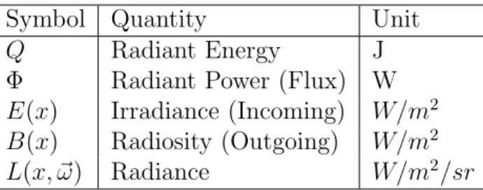
Symbol Quantity Unit
Q Radiant Energy J
Φ Radiant Power (Flux) W
E(x) Irradiance (Incoming) W/m2
B(x) Radiosity (Outgoing) W/m2 L(x, ~ω) Radiance W/m2/sr
Table 2.1: Common radiometric symbols, terms and units. x is a specific surface point. Radiance may be either incoming or outgoing depending on the direction of ~ω.
measured in Watts (W) (Joules per second) and referred to as radiant power orflux.
Φ = dQ
dt
A light source, such as a household light bulb, can be described as emitting a certain number of Watts1. In a similar fashion, the rate at which photons arrive on an office
desk from all directions is a measure of flux.
To describe the movement of light energy over time at a specific point, x the flux is differentiated over an area and is measured in Watts per square meter. This unit is referred to as radiosity, B(x), if the light is being emitted and irradiance, E(x), is the light is incident. The term irradiance is an unfortunate historical artifact as it is not the opposite of radiance, defined shortly.
E(x), B(X) = dΦ
dm2
Radiosity does not distinguish the direction that light was traveling when measured and is therefore unsuitable for making critical measurements such as the amount of light arriving at a camera from a particular angle.
1Light bulbs are labeled by the electrical energy they consume over time, also measured in Watts.
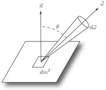
Figure 2.3: Radiance is the total radiant flux arriving across, or departing from, a differ-ential area from the range of directions in a differdiffer-ential solid angle around ~ω. Depending on the direction of light transport, radiance is categorized as incident or exitant. Radi-ance is the physical unit measured by image sensors such as eyes and cameras.
Radiance, L(x, ~ω), is the flux across a differential area from a specific differential direction (solid angle) and is measured in Watts per square meter per steradian (Fig-ure 2.3).
Li(x, ~ω) =
d2Φ
dm2dω
Radiance may be either incident, Li(x, ~ω), emitted, Le(x, ~ω), or reflected, Lr(x, ~ω). The
exitant radiance is the sum of the emitted and reflected radiance, Lo(x, ~ω) =Le(x, ~ω) +
Lr(x, ~ω). Image sensors, such as our eyes, cameras, and virtual cameras, are modeled as
sensors of radiance. Radiance also plays a critical role in the modeling of reflection and refraction on non-diffuse surfaces.
Figure 2.4: The invariance of radiance. The exitant radiance leaving a point in the direction of another is exactly equal to the radiance arriving at second point from the direction of the first.
in a straight line to form an important property of radiance. As shown in Figure 2.4, the exitant radiance at point x in the direction ~ωo towards point y is equal to the radiance
that arrives at y from the direction, ~ωi of x.
Lo(x, ~ωo) = Li(y, ~ωi)
This critical property allows us to compute the incident radiance at a point if we already know the exitant radiance at other points in the scene. This observation forms the basis of the rendering equation.
2.3.2
The rendering equation
Image
Plane Pinhole Object
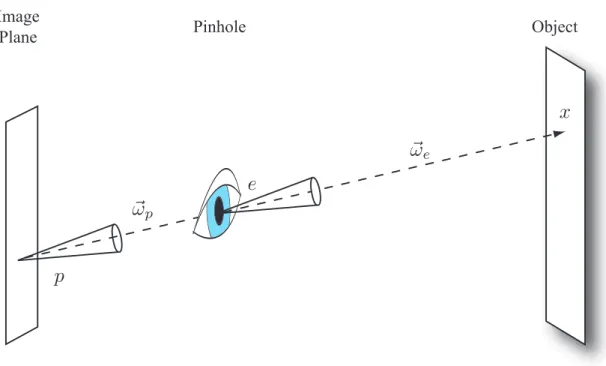
Figure 2.5: Image formation with an ideal pinhole camera. For every pixelpin the image, the radiance arriving at the eye-point e from x in the direction ~ωp must be computed.
Li(e, ~ωp) =Lo(x,−~ωp)
enable additional visual effects. Because the pinhole allows only one ray of light to reach any point on the image plane, it is the incident radiance, Li(p, ~ωp), that is measured.
By the invariance of radiance, this is the same radiance passing through the pinhole, at position e, along the same ray~ωp. The position e is commonly referred to as the camera
location or eye-point. The ray originating at e in the direction ~ωp is called an eye-ray.
Each eye-ray must be intersected with the scene to find the first intersection point,
Pre-condition: e is the location of the eye (camera)
Pre-condition: Any per-scene or per-image pre-procesing has been performed for each pixel (u, v) of the imagedo
for each sample do image(u, v)←0
// Form the eye-ray (e, ~ωp)
p← sampled location on the image plane of pixel (u, v)
~
ωp ←(e−p)
// Use ray-casting to find the closest intersection in the scene
x←intersect with scene(e, ~ωp)
// ComputeLi(e, ~ωp) based on Lo(x,−~ωp)
image(u, v)←compute exitant radiance(x,−~ωp)
end for
image(u, v)←image(u, v)/(# samples) end for
Post-condition: image = the generated image
Algorithm 2.1: The pixel-driven rendering algorithm, adapted from (Dutr´e et al., 2003). The quality of a generated image depends on the exact implementation of the method compute exitant radiance().
radiance at x back along~ωp.
Li(p, ~ωp) = Li(e, ~ωp) =Lo(x,−ω~p)
Algorithm 2.1 provides a high-level view of this process, deferring for the moment how the exitant radiance, Lo, is computed.
The exitant radiance at x towards the eye, or any other point in the scene viewed from a particular direction, is the sum of the reflected, refracted and locally emitted radiance. The emitted radiance, Le, is computed directly from the description of the
from a potentially different point, z0, in a potentially different direction, ~ωo. When
restricted to reflection2 this is known as the Bidirectional Scattering Surface Reflectance Distribution Function (BSSRDF) and has eight dimensions (Nicodemus et al., 1977).
Nicodemus also introduced a simplification of the BSSRDF where reflected light is assumed to be emitted from the same location where it landed (z0 =z). The Bidirectional Reflectance Distribution Function (BRDF) is denoted as
fr(z, ~ωi, ~ωo) =
dLr(z, ~ωo)
Li(z, ~ωi)(ω~i•~n)d~ωi
where ~ωo is towards the viewer, ~ωi is the direction from which the incoming light is
arriving, ~n is the local surface normal at z, Lr is the reflected radiance towards the
viewer, and (ω~i•~n) represents the foreshortening due to the two surfaces not necessarily
being parallel. Although this formulation precludes the representation of some desired visual effects, such as the sub-surface scattering seen in white marble statues, it can be computed without additional expensive pre-computation.
The perfectly specular BRDF, an ideal mirror, reflects the incoming light energy only along the reflected angle and is a special case. The BRDF of a more general surface will reflect some portion of the incoming light to the entire hemisphere of visible directions. Purely diffuse surfaces reflect the light evenly, while glossy surfaces exhibit a behavior between that of ideal specular and diffuse reflectors. Some examples of common BRDFs are illustrated in Figure 2.6. Global illumination algorithms differ in the BRDFs that they efficiently support.
The concepts of incident, reflected and emitted radiance and the BRDF are united in the rendering equation (Kajiya, 1986) using an integral with a domain of the hemisphere,
2Refraction can be analyzed in a symmetric fashion to reflection. For clarity, refraction is not
Figure 2.6: Examples of common BRDF classifications. The purely diffuse BRDF reflects light from all directions equally towards the viewer, while the highly specular surface, an ideal mirror, reflects only the light from a single direction. In between, glossy surfaces reflect light from all directions, but weigh those that come near the angle of specular reflection more heavily.
Ω, of incoming radiance at z and shown in Equation 2.1.
Lr(z, ~ωo) =Le(z, ~ωo) +
Z
Ω
fr(z, ~ωi, ~ωo)Li(z, ~ωi)(~ωi•~n)d ~ωi (2.1)
2.3.3
Numerical integration
The integrand of the rendering equation, shown in Equation 2.1, is the complicated product of three separate functions. The incident radiance function, Li(x, ~ω) is
gener-ally unknown3 and exhibits strong discontinuities because of changes in visibility. For
these reasons, analytical integration can not be applied to the rendering equation. The approach of this section is inspired by (Veach, 1997).
When an integral can not be solved analytically in closed form, Equation 2.2, nu-merical integration can be used to find an estimate, ˆΘ, of the true value Θ (Hamming, 1973). The integral is replaced by the weighted sum of N discrete point evaluations of the integrand, g(s), as shown in Equation 2.3. There are an entire family of numerical integration estimators that differ in their selection of the pointsSi at whichg(s) is
eval-uated and the weights Wi which describe how they are combined. The correctness and
efficiency of these techniques depends on the exact function being integrated. In the case of computer graphics and the rendering equation, many techniques are not suitable.
Θ =
Z
Ω
g(s)dµ(s) (2.2)
ˆ Θ =
N
X
i=1
Wig(Si) (2.3)
The rendering equation, g(s) = fr(x, ~ωi, ~ωo)Li(x, ~ωi)(~ωi•~n) is the product of three
functions, with x and ~ωo fixed. The domain of integration, Ω, is the entire hemisphere
of directions from which light arrives at x. Each sample Si is a single direction light
may be arriving from. dµ(s) is the differential solid angle and Θ is the reflected radiance reflected for which we are solving.
As a point of notation, statisticians customarily refer to each value Si as an
obser-3Indeed, if Li(x, ~ω) were known for allxand~ω, then an evaluationLi(e, ~ωp) for all eye-rays would
vation and the entire vector < S1, S2, S3,· · ·SN > as a sample. In computer graphics
it is standard to refer to each observation Si as a sample and call N the sample size.
The whole vector of samples is informally referred to using a variety of terms such as “sample locations” or in the case where Ω is the hemisphere, “sample directions”. In this dissertation, the computer graphics terms are used exclusively.
A simple numerical integration technique used in introductory Calculus courses is the Riemann Sum. The samples Si are spread uniformly throughout the domain Ω.
Each sample is given a weight Wi = N1. The Riemann Sum is a deterministic numerical
integration technique because the sample locationsSi and weightsWi are fixed ahead of
time.
Other deterministic integration methods include the trapezoid rule and Simpson’s rule. Although beneficial in other domains, these methods are rarely useful in computer graphics because unless the integrand is smooth, a very large sample size will be re-quired to achieve good results (Veach, 1997). Even more troublesome, extending these techniques to more than one dimension is very expensive. If N samples are sufficient for a given one-dimensional problem, Nd samples would be required for a d-dimensional
problem. This is known as the “curse of dimensionality”.
2.3.4
Monte Carlo integration
In contrast to these deterministic methods, Monte Carlo integration is stochastic. The samples, Si, are chosen randomly from the region of integration, Ω. The generic Monte
Carlo estimator of g(s), GN, is shown in Equation 2.4 (Rubinstein, 1981). Since all the
weights in Monte Carlo estimators have a common term of N1, this has been factored out of the summation.
GN =
1
N
N
X
i=1
If Wi = 1 and every point in Ω has the same probability of being sampled by Si
then this is called the Blind Monte Carlo technique. Although Blind Monte Carlo is very straightforward, samples are chosen from the domain randomly but uniformly, it takes a large value of N to have much confidence in the estimate. Importance sampling is one technique to improve the performance of the blind Monte Carlo estimator, and is discussed in detail in Chapter 6.
To apply Monte Carlo integration to the rendering equation, Equation 2.2, the po-sition x and the viewing angle ~ωo are fixed. Instead of integrating over the continuous
hemisphere Ω, the hemisphere is discretely sampled and the results summed as in Equa-tion 2.5.
Lr(x, ~ωo) = Le(x, ~ωo) +
1
N
N
X
i=1
fr(x, Si, ~ωo)Li(x, Si)(Si•~n) (2.5)
2.4
Global Illumination algorithms
2.4.1
Path tracing
Path tracing algorithms establish light transport paths between lights sources and those points in the scene where we wish to compute the incident radiance. Often, these points are directly on the image plane, corresponding to the pixels of the rendered image. This approach yields the pixel-driven rendering algorithm presented in Algorithm 2.1. The path tracing methods differ in their implementation of compute exitant radiance(x, ~ωo)
and any preprocessing that may be required before image generation begins.
2.4.1.1 Whitted-style ray tracing
Perhaps the best known path tracing algorithm is ray tracing, introduced to computer graphics by Whitted (Whitted, 1980). Requiring no pre-processing and being fully de-terministic, the method is simple to implement (Algorithm 2.2). The desired exitant radiance is computed as the sum of three terms: the locally emitted light, the reflected light due to direct illumination from the scene-defined light sources, and the light reflected along the angle of perfect reflection or refraction. The integral in the rendering equation is replaced with one recursive evaluation of compute exitant radiance computing indirect illumination.
Pre-condition: x is the location under consideration Pre-condition: ~ωo is the direction towards the viewer
// Compute the locally emitted radiance in direction~ωo
result←emitted illumination(x, ~ωo)
// Compute the direct illumination due to the pre-defined light sources result←result + direct illumination(x, ~ωo)
// Compute the indirect illumination due to specular reflection if recursion termination criterion not yet reachedthen
~
ωi ←compute reflected angle(~n, ~ωo)
y←intersect with scene(x, ~ωi)
result←result +fr(x, ~ωi, ~ωo)×compute exitant radiance(y,−~ωi)
end if
Post-condition: result = the total reflected radiance from xtowards ~ωo
Algorithm 2.2: Whitted-style ray tracing. Various heuristics can be used to terminate recursion. This simple implementation of compute exitant radiance(x, ~ωo) is valid only
for perfectly specular surfaces, such as chrome balls. Nonetheless, it provides impressive results in suitable scenes.
2.4.1.2 Stochastic ray tracing
Cook introduced distributed ray tracing as a comprehensive framework for extending Whitted-style ray tracing using stochastic techniques, based on Monte-Carlo integra-tion (Cook et al., 1984). It handles arbitrary material BRDFs, as well as mointegra-tion blur, depth of field, and other realistic effects. In a straightforward implementation, arbitrary BRDFs are supported by replacing the single reflection sample, along the angle of specu-lar reflection, with N randomly chosen samples using Equation 2.5 to compute the total reflected radiance. These random samples can be chosen uniformly, proportionally to the BRDF, or according to the quasi-Monte-Carlo technique (Shirley, 2000). Even an implementation of this basic technique that allowed only 4 levels of recursion, generating seriously biased images, would require N4 evaluations of compute exitant radiance. As
N is in the range of hundreds to thousands, this implementation of distributed ray trac-ing is highly inefficient, but can be easily adapted to preserve its strengths while reductrac-ing the number of computations that contribute little to the final image.
Pre-condition: x is the location under consideration Pre-condition: ~ωo is the direction towards the viewer
// Compute the locally emitted radiance in direction~ωo
result←emitted illumination(x, ~ωo)
// Compute the direct illumination due to the pre-defined light sources result←result + direct illumination(x, ~ωo)
// Determine if recursion should continue
ρ←probability of absorption if ρ > random unit number then
// Compute the indirect illumination due to specular reflection
~
ωi ←sample visable hemisphere(~n, ~ωo)
y←intersect with scene(x, ~ωi)
result←result +fr(x, ~ωi, ~ωo)×compute exitant radiance(y,−~ωi)/(1−ρ)
end if
Post-condition: result = the total reflected radiance from xtowards ~ωo
Algorithm 2.3: Stochastic ray tracing. Using Monte Carlo integration to support ar-bitrary BRDFs and Russian roulette to terminate the recursion, stochastic ray tracing is a simple but robust global illumination algorithm. Because only a single sample is generated and evaluated, many samples per pixel must be generated from the image plane.
2.4.1.3 Additional path tracing algorithms
Although more expressive than Whitted-style ray tracing, stochastic ray tracing has the problem that many of directions sampled will contribute little towards the final image unless they are directed to those portions of the scene that either contain light sources or strong reflectors of light sources. This results in a noisy image, especially if any caustics are present. Two alternative path tracing techniques increase efficiency by utilizing the knowledge of the specified light sources.
Bi-directional path tracing, like stochastic ray tracing using Russian roulette, traces
multiple rays from the eye deep into the scene, recording all the intersection points (Lafor-tune and Willems, 1993; Veach and Guibas, 1994). Rather than using shadow rays to compute direct illumination and propagating backwards through the ray, a second ray is traced from a light source, recording all its intersections. Using the visibility function, as determined by ray tracing, and a series of weights, derived from the rendering equation, the light power is transfered from the light ray to eye ray and accumulated at the pixel. Although each eye ray is significantly more expensive to process, in certain scenes it can take far fewer samples per pixel to reduce noise to an acceptable level.
2.4.2
Radiosity
Classical radiosity computes a radiosity value for every surface point in the scene dur-ing a view-independent pre-process (Goral et al., 1984). The surfaces in a scene are divided into patches and initialized with the appropriate radiosity if the patch is part of a light source. Using a numerical linear system solver, the energy is allowed to transfer through the system until a steady state is found. This solution is then consulted by compute exitant radiance() directly during pixel-driven rendering, Algorithm 2.1. Based on energy balance equations from radiative heat transfer studies, radiosity has been val-idated to direct physical observation (Goral et al., 1984; Pattanaik et al., 1997). Recall that the radiometric term radiosity describes the total flux leaving a differential point in all directions. By not storing the hemispherical distribution of exitant radiance, the standard method can only support scene that are purely diffuse.
A significant amount of research has been published on improving the computational efficiency of radiosity, removing artifacts due to the selection of the patches and extending the technique to non-diffuse surface. These results are well summarized in (Cohen and Wallace, 1993) and (Dutr´e, 1994, Chapter 5). Unfortunately, some difficulties remain. The surfaces must be parameterizable in order to be divided into patches, adding com-plexities when arbitrary procedurally generated geometry is used. Additionally, many of the techniques to improve efficiency remove the regularity of operations and make it dif-ficult to take advantage of parallel independent processors with limited communication.
2.4.3
Discussion
illumi-nation algorithm for a given use are:
• The restrictions imposed on the scene, both geometric and material properties
• The visual effects that are correctly and efficiently rendered
• The computation required to prepare intermediate data structures
• The ability to parallelize the workload on cost effective architecture
None of the algorithms examined so far in this chapter meet these requirements for the scenes and visual effects described in Chapter 1. In Section 2.6 photon mapping is presented as a possible contender implementation in fifth generation graphics hardware. The next section examines existing fifth generation graphics architectures, focusing on those that are used by or inspired the architecture presented in Chapter 7.
2.5
Fifth generation graphics architectures
As described in Section 2.1, it is expected that fifth generation graphics architectures will concentrate on adding support for global illumination. There is as of yet no com-mercially available examples of interactive4 fifth generation architectures, however there
are research designs that have been proposed and/or built. Many early hardware global illumination systems are discussed by Chalmers (Chalmers et al., 2002). In this section I discuss a sample of the more recent system architectures intended to be implemented as interactive hardware, that have inspired aspects of the architecture presented in this dissertation.
A series of papers and prototype machines from the University of Saarland define an efficient architecture for interactive ray tracing. The original SaarCOR design required
4The RenderDrive line of products by ARTSVPS are commercially produced offline accelerators for
a static scene and only supported a limited numbers of secondary rays (Schmittler et al., 2002). A highly efficient FPGA implementation demonstrated that the architecture was able to operate with very limited memory bandwidth by tracing rays in small bun-dles (Schmittler et al., 2004). More recently, a second implementation with partially dynamic scenes and programmable shaders with more secondary rays has been demon-strated (Woop et al., 2005). The architecture is still however a Whitted-style ray tracing, unable to efficiently handle diffuse inter-reflections, caustics, or other phenomena that the photon mapping algorithm handles well.
As described in Section 2.6, ray casting is one of the two most important compu-tational kernels in photon mapping. The SaarCOR architecture casts coherent rays in order to reduce the required memory bandwidth significantly. The algorithms deployed in the architecture described in Chapter 7 take care to ensure coherency of not only the photon gather locations, but also the rays that are cast using a small instantiation of the SaarCOR.
The GI-Cube architecture provided Whitted-style ray tracing in the context of volume rendering (Dachille and Kaufman, 2000). The regular nature of the volume rendering allowed for a simple packet based routing structure to sort partially traced rays to im-prove cache coherencey. This provided both inspiration for the hashed photon gather reordering presented in Chapter 3 as well as the overall packet-based routing for the entire architecture presented in Chapter 7.
2.6
Photon mapping
geometric primitives, as was demonstrated in Figure 1.1. When these visual effects are present in an image, photon mapping tends to be cheaper than the previously discussed alternatives for images of equivalent variance. It is however important to note that the algorithm is biased. Once the photon map is generated, the final image will not reach zero variance as the number of pixel samples increases to infinity. The algorithm generates an image in two phases.
The first phase breaks the energy of the light sources into discrete packets called pho-tons. Although inspired by the physics of light, this use of the word photon is somewhat
misleading because they do not represent actual physical photons. The name is how-ever highly suggestive of the initial algorithm and has become entrenched. The photons are shot into space and allowed to probabilistically reflect, refract and be absorbed by surfaces. At every intersection with the scene, the photon, their locations, energy, and direction of travel, are recorded in the photon map.
The actual image is generated in the second phase. The photon map is an estimate of the incident radiance at any point in the scene. To consult the photon map, a photon gather is performed. This is essentially a kNN search, using the photon map to find the
k photons closest to the point of interest. The photon gather is used to terminate, at an early stage, the recursive evaluation of rendering equation.
The photon map algorithm is most comprehensively described in Jensen’s own book with pointers to more recent research (Jensen, 2001). In this section, we examine more closely the two phases of the algorithm and examine the costs to determine what the limiting factor is.
2.6.1
Photon map creation
Pre-condition: NP M is the number of photons requested for the indirect photon map
while #Photons< NP M do
// Determin initial photon position and direction
p←position on a light source
~
d←randomly selected direction from light source // Follow photon through scene until absorbed caustic path ← true
repeat
x←intersect with scene(p, ~d)
if x is not a highly specular surface then caustic path ← false
Record (x, ~d) in the indirect map end if
if caustic path is true then
Record (x, ~d) in the caustic map end if
p← compute reflected angle(x,−d~) until photon is absorbed
end while
Post-condition: The indirect and caustic photon maps represent a sparse representa-tion of incident radiance throughout the scene
Algorithm 2.4: Photon map creation. Photons are traced from the light sources through the scene. The intersections are recorded in the indirect photon map. The caustic photon map records only those intersections which were not diffusely reflected from the light. The process continues until enough photons are successfully traced.
the initial direction from the light sources into the scene. Each photon is then traced through the scene (Algorithm 2.4). They are probabilistically reflected, refracted and finally absorbed at diffuse or glossy surfaces. A record, p, is made of each intersection the photon has with the scene. Only those intersection with highly specular surfaces are not stored. It is these records that form the entries in the photon map, storing the location, xp, attenuated flux, Φp, and incident direction, ~ωp. A second, smaller, photon
For typical scenes with indirect illumination, the number of photons shot, NP M, is
required to be in the hundreds of thousands or even millions (Jensen, 2001). As there will be a very large number of kNN searches, it is important that these searches be efficient. The standard acceleration data structure is the kd-tree (Bentley, 1975). The choice of data structure will be studied in Chapter 4.
For static scenes the photon map can be generated as a single preprocess and reused for multiple viewpoints. Alternatively, time dependent photon mapping adds time as dimension for thekNN gathers, allowing for animations without temporal aliasing (Cam-marano and Jensen, 2002). Jensen described a simple three-pass technique that uses an additional importance map, generated by shooting importans (Jensen, 1996b). Impor-tans are an analogue of photons; they are shot from the camera into the scene and their distribution is then used to determine when the standard photons should be recorded in the photon map. Additionally, importance sampling can be used to guide the initial di-rections in which photons are shot using a projection map from the light sources (Jensen and Christensen, 1995).
2.6.2
Image generation
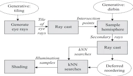
After the photon maps are created, the image is rendered using the pixel-driven al-gorithm (Alal-gorithm 2.1). The exitant radiance is computed in four steps, outlined in Algorithm 2.5. The direct and emitted illuminations are computed in the same manner as they were for path tracing. The indirect illumination however is computed twice, once for general indirect illumination and once for caustics, using the two separate photon maps.
Pre-condition: x is the location under consideration Pre-condition: ~ωo is the direction towards the viewer
// Compute the locally emitted radiance in direction~ωo
result←emitted illumination(x, ~ωo)
// Compute the direct illumination due to the pre-defined light sources result←result + direct illumination(x, ~ωo)
// Compute the indirect illumination using the caustic photon map result←result + photon gather(caustic map, x, ~ωo)
// Compute the indirect illumination using the indirect photon map result←result + compute indirect(x, ~ωo)
Post-condition: result = the total reflected radiance from xtowards ~ωo
Algorithm 2.5: Generation of an image using the photon map. Direct illumination and self emitted radiance are computed as they were for path tracing. The caustic photon map is queried using a single photon gather. The rest of the indirect illumination is computed using one of the two visualization techniques discussed in this section.
sampling of the incident radiance at the position x, Jensen showed that the rendering equation can be adapted to compute the reflected radiance at x in any direction, Equa-tion 2.6, without further recursion of the rendering equaEqua-tion. (The term A represents the area of the circle defined by the radius required to find all k photons.) This process is referred to as a photon gather and is illustrated in Figure 2.7. It is worth noting that this process is similar to Monte Carlo integration, except that the sample directions have been chosen previously, by the selection of photon paths.
Lr(x, ~ωo) = k
X
p=1
fr(x, ~ωp, ~ωo)
4Φp(x, ~ωp)
4A (2.6)
Figure 2.7: Computing reflected radiance using a photon gather. A single photon gather performed at x to estimate the reflected indirect illumination. Thek nearest photons in the photon map are located, and are interpreted as a sparse representation of the incident radiance, allowing for the evaluation of the rendering equation without further recursion.
2.6.2.1 Final gather visualization
The final gather visualization, shown in Figure 2.8, estimates the reflected radiance at x
by evaluating the rendering equation using a Monte Carlo integration. Instead of a single photon gather, the hemisphere surrounding x is sampled and N rays, ~ωi, are cast out
into the scene as described in Section 2.3.4. At each intersection point, yi, a standard
Figure 2.8: Final gather visualization of the photon map. A higher quality estimate of incident radiance is obtained by using Monte Carlo integration to perform a final gather. A photon gather is performed at the end of each secondary ray, ω~i.
2.6.3
Computational Requirements
The computational requirements of generating interactive images using the final-gather visualization algorithm are significant. The costs are analyzed in Section 7.3 and sum-marized in Section 7.3.5. The most significant portion of the computation is the indirect photon gathers. The photon gathers require a kNN search (traversing the photon map, comparing normals and verifying that the photons found are within the allowed radius), evaluating the BRDF for each photon chosen, and finally the accumulation in the frame buffer of the results.
is expected to be available on CPUs in the near future. In Section 2.2 it was estimated that fine-grained graphics applications can easily expect to support 500 GFLOPS of computation by 2010. The workload of the Sponza atrium would need to be split among 13 chip replications to achieve this rate. This number of chips, each with dedicated high-speed memory, is aggressive to include within a single host workstation.
2.6.4
Bandwidth Requirements
The bandwidth requirements of photon mapping are measured as either the total number of bytes that must be transfered from off-chip memory to render an image, or as a rate using the number of bytes per second. The data structures holding the photon map, geometry, surface properties and other required items are too large to fit in embedded memory for the next several years.
The modified Cornell box image in Figure 1.2 requires 50 GB to render, or 1.4 TB/s at 30 frames per second. The Sponza scene requires 367 GB per image, or 11 TB/s at 30 frames per second. These bandwidth rates are very high, with the bulk of the cost due to the kNN searches for the indirect photon gathers. Using the estimate of near future memory bandwidth in Section 2.2, the 11 TB/s would require that the workload be divided among 123 chips each with a replication of the same memory. This is not feasible to house in a single host workstation, and would require either a large cluster or a large specially built chassis.
2.7
Discussion
CHAPTER 3
PHOTON GATHER REORDERING
Rendering an image with the naive photon mapping algorithm, as described in Sec-tion 2.6, generated a tremendous amount of memory traffic. The Sponza scene, for example, required 367 GB for a single image. An interactive system generating thirty frames per second would therefore require at least 11 TB/s of memory bandwidth. Only a small portion of the required bandwidth can be attributed to solving the visibility problem, with ray casting, or performing the local evaluation of surface reflectance, in the form of texture lookups. The large value is due almost entirely to the photon gathers. Chapters 5 and 6 will describe two techniques to reduce the number of photon gathers that must be performed, and thus indirectly the bandwidth requirements. Together with Chapter 4, this chapter focuses on reducing the bandwidth costs of performing a particular and fixed set of photon gathers without any modifications to the generated image. This is achieved by changing the order of operations, allowing the memory cache to become more effective.