THE INTERGENERATIONAL TRANSMISSION OF EDUCATIONAL ATTAINMENT REVISITED: THE EFFECTS OF SOCIOECONOMIC BACKGROUND, GENETIC
INHERITANCE, AND COHORT
Meng-Jung Lin
A thesis submitted to the faculty at the University of North Carolina at Chapel Hill in partial fulfillment of the requirements for the degree of Master of Arts in the Department of
Sociology in the College of Arts and Sciences.
Chapel Hill 2017
Approved by:
Guang Guo
Ted Mouw
ABSTRACT
Meng-Jung Lin: The Intergenerational Transmission of Educational Attainment Revisited: The Effects of Socioeconomic Background, Genetic Inheritance, and Cohort
(Under the direction of Guang Guo)
This research revisits the intertwined social and biological pathways of the
intergenerational transmission of educational attainment. By estimating the effects of the
whole-genome genetic variants by the continuation ratio logit regressions using 8,251
samples from the Health and Retirement Study (HRS), and considering for socioeconomic
status in childhood on education at the same time, I first examine the relative individual
impacts of biological and social influences. Then, I consider how parental education shapes
the expression of the genetic potential by including moderating effects between the two.
Finally, I explore the curvilinear trend of genetic effects over time, and use cohort separated
models to investigate the decline in the moderating effects of parental education on
educational attainment. The findings suggest the influences are from both genes and family
socioeconomic background. Also, the genetic effects were not only negatively moderated by
socioeconomic background, but changed curvilinearly over time corresponding to the
expansion of higher education in the mid-twentieth century in the U.S. The pattern indicates
the educational opportunities equalized at first but saturated after higher education became
more accessible. This study furthers the understanding of the social mobility process and
TABLE OF CONTENTS
LIST OF TABLES……….………vi
LIST OF FIGURES………...vii
INTRODUCTION………..…1
BACKGROUND………...5
Educational Attainment and Social Mobility……….5
The Integration of Biological Accounts……….6
Historical Changes and Genetic Effects on Educational Attainment………...14
DATA AND METHODS………..19
Data………...19
Variable Measurement...………20
Analytic Strategy………..………23
RESULTS……….28
Descriptive Statistics………28
Continuation Ratio Models Predicting Educational Attainment………...30
Cohort Differences………...35
Predicted Probability………38
CONCLUSION AND DISCUSSION………..42
APPENDIX A: UNCONSTRAINED CONTINUATION RATIO MODEL………..49
APPENDIX B: RESULTS FOR 73-SNPS POLYGENIC SCORE……….51
APPENDIX D: GREML RESULTS………..61
LIST OF TABLES
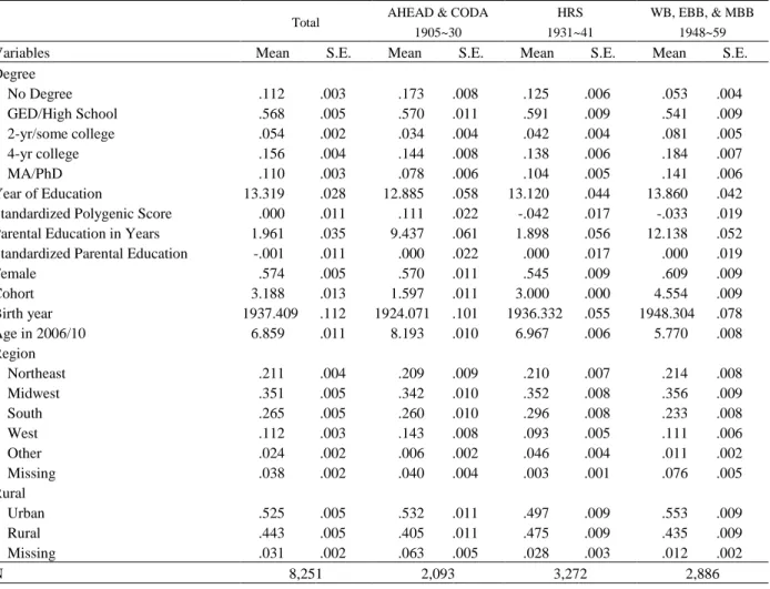
Table 1. Descriptive Statistics for Full Sample and Different Cohorts………29
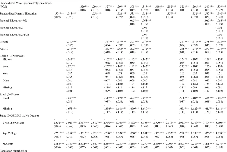
Table 2. Continuation Ratio Model Predicting Educational Attainment………...32
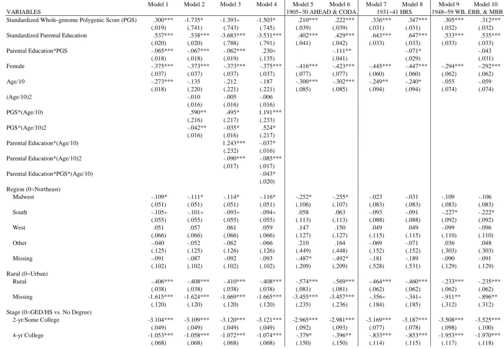
Table 3. Cohort Differences in Continuation Ratio Model Predicting
LIST OF FIGURES
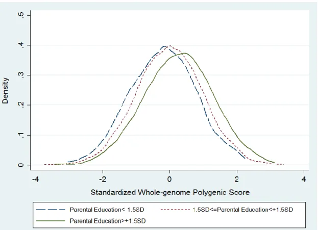
Figure 1. Correlation between the Standardized Parental Education and
Offspring’s Standardized Whole-genome Polygenic Score for Education………….30
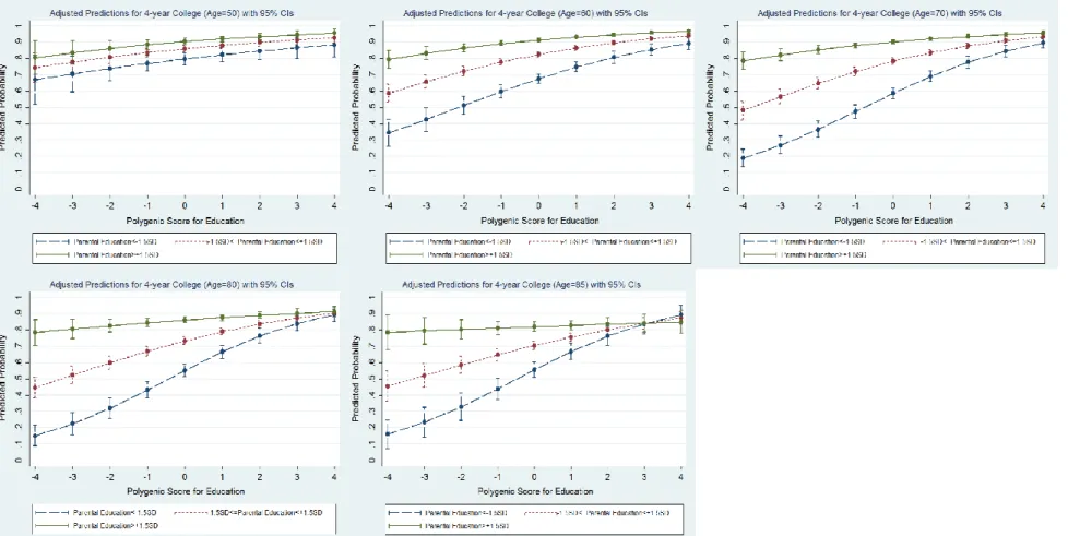
Figure 2. Predicted Probabilities for Advancing into a 4-year College by
Holding Covariates at Means………..39
INTRODUCTION
In the U.S., children born to the families in the poorest 20 percent of the income
distribution have barely about 9 percent of chances to rise to the richest 20 percent as adults
for the last two generations (Chetty et al. 2014). While the figure remains stable for the
1970-80s birth cohorts, recognition of the unequal intergenerational mobility of the U.S. society
has increased lately. The upward and downward intergenerational mobility occurs depends
largely on both parental and children’s educational attainment (Blau and Duncan 1967).
However, although social scientists interpret the transmission of educational attainment
mainly through social inheritance, it is arguable that genetic heritability also plays a role in
the mobility process (Eckland 1967; Duncan 1968; Behrman and Taubman 1989; Jencks and
Tach 2006; Nielsen 2006; Nielsen and Roos 2015). Failure to discern social and biological
pathways leads to a weak standpoint for sociologists’ belief that the transmission of
educational achievement operates socially from family backgrounds, and it may simply
represent the effects of a genetic predisposition underlying the process. Past studies using
twins and siblings to address the issue were not able to account for the specific genetic effects
due to the unclear identification of the shared genes, and the difficulties to distinguish genetic
effects from environmental effects because the identical twins are more likely to pursue alike
environment more than fraternal twins do. Therefore, by incorporating the polygenic score of
education, a measure that summarizes the effects of specific genetic variants that are
associated with education, this study attempts to answer the question directly.
To sociologists, distinguishing both social and genetic pathways could illuminate
sociological research, but it also helps to facilitate the examination of how environment
shapes the expression of the genes. The realization of the genetic potential, which refers to
the actualization of the innate ability, can be considered as a signal for the equalization of
opportunities to attain higher education. When the environment provides individuals with
appropriate resources, their genetic potential can actualize more fully than when the resources
are barren. For example, in terms of proximate surroundings, family backgrounds might limit
or encourage the full achievement of the genetic predisposition. Several hypotheses have
been proposed for the gene-environment interaction pattern on status-related outcomes
(Nielsen 2016). The directions of the moderating effects of the environment can be positive
(Scarr-Rowe hypothesis), curvilinear (Pareto hypothesis), or negative (Saunders hypothesis)
under different circumstances. When families with high status are able to encourage the
genetic effects of their offspring and it is not the case for the low status families, the
Scarr-Rowe hypothesis is supported, whereas when these high status families are merely able to
protect their offspring from downward mobility and the genetic effects express more fully for
the low status families, the Saunders hypothesis is evidenced. Somewhere in between, the
Pareto hypothesis would be true if both the highest and the lowest status are crystallized, and
the middle class is the only class to mobile. Empirically, studies mostly support the
Scarr-Rowe hypothesis. A case would be the children from disadvantaged backgrounds often suffer
from the constrained chances to fulfill their potentials (Guo and Stearns 2002). However,
since studies have seldom tested these alternative hypotheses, this paper will examine them
using the interaction terms between the family backgrounds and the genetic polygenic score.
Also, with regard to the macro environment, historical changes could suppress or
enhance the genetic effects on attainment. Research has shown that as educational policies
became liberal in the second half of the twentieth century, genetic potential turned out to be a
universal access to higher education might contribute to the weaker genetic effects for the later
born cohorts (Okbay et al. 2016). The inconsistent findings can be reconciled by considering the
genetic effects changed curvilinearly through the expansion of higher education. If the
curvilinear genetic effects have synced with the declining or the inverted U-shaped effects of
family socioeconomic status and their downward moderating effects on genes over time, these
would suggest an equalization process during the time. In contrast, if the family socioeconomic
status effects increase, the reducing genetic effects and growing family backgrounds effects
depict an unequal society in development.
In this study, I will examine both the moderating effects of family backgrounds and
historical changes on the relationship between genetic variants and educational attainment. Since
the United States has undergone the expansion of higher education gradually and stably in the
twentieth century, and the sample I use constituted of adults above age 50, they could have
experienced the growing opportunities to obtain higher education to different extents if they were
born in different periods of time. The loosening constraints of attaining higher education might
thus result in the better likelihood of realizing their genetic potential for education in the younger
cohorts within these old adults. At the same time, the saturation of higher education which refers
to the lower thresholds to entering college education would also be possible to reduce the effect
of genes.
This study uses the nationally representative data of older adults from the Health and
Retirement Study (HRS) to examine three related issues on educational attainment by applying
the polygenic scores constructed from the recently GWAS results (Okbay et al. 2016). First, I
examine the relative magnitude of the effects of social inheritance and genetic heritability on
of genetic potentials and which gene-environment interaction hypothesis on educational
attainment is supported. Third, to understand whether the U.S. society equalized or became
unequal in the mid-twentieth century, by considering cohort differences further, I test the
argument that historical changes influence the structural opportunities for individuals to achieve
their genetic potentials, and the changing effects of family socioeconomic status over time. The
study can contribute both academically and publicly by providing new insights into to the
long-lasting issue of social mobility, and advising how public policies can help to equalize the
BACKGROUND Educational Attainment and Social Mobility
Individuals possess two statuses, ascribed status and achieved status, which also describes
the processes through which one obtains position in society. Ascribed status refers to the status
individuals are born with. For example, gender, ethnicity, genetic predisposition, parental
education, and family socioeconomic status, are all determined before their birth and can rarely
be changed. In contrast, achieved status is the status that is achieved by the individual.
Achievements such as educational and occupational attainment are considered achieved statuses.
In this distinction, sociologists often consider the realization of the latter as an indicator of social
mobility in the society. Along the same lines, Blau and Duncan’s (1967) seminal status
attainment model demonstrates the paths among ascribed statuses and achieved statuses. Their
analysis illustrates how a father’s education and occupation are influential factors in the
respondent’s educational and occupational attainments, and thereby highlights the effects of the
ascribed status on social mobility. However, Blau and Duncan still argued that, “(self-)education
operates primarily to induce variation in occupational status that is independent of initial status (pp.203),” which maintains the role of education as an equalizer that ameliorates the
reproduction of social status. While the “vicious cycle” of reproducing social status across
generations might not be true, and education might be an equalizer, it is confirmed that parental
education and occupation are important factors in their offspring’s attainments. Nevertheless, it
Studies have been done to understand this black box. Soon after Blau and Duncan (1967),
the Wisconsin Model tried to explain the intergenerational transmission of educational attainment
by taking social psychological variables into account, such as the influence and aspirations of
significant others (Sewell, Haller, and Portes 1969). Using a broader framework, Jonsson et al.
(2011) provides a set of mechanisms analyzing intergenerational reproduction of occupation,
which is tightly linked with education. Under their framework, four kinds of resources underlie
the mechanisms: human capital, cultural capital, social network, and economic resources. Human
capital includes the cognitive skills and abilities the class members share and the families have.
Cultural capital refers to the culture and taste enjoyed by the class, and the aspirations from
parents. Social network indicates the social ties that the neighborhoods and family members
own, which can possibly connect to better resources. And economic resources are the incomes
and businesses the class and the families have. By transmitting all of these resources to children,
parents reproduce their advantage or disadvantage in the next generation.
Although these studies have established abundant accounts for the reproduction of
education, their explanations are often built upon the assumption that ascribed statuses transmit
effects socially. That is, only through resources can ascriptive characteristics other than genetic
predisposition affect achieved statuses. However, biological heritability between parents and
children also connects parents’ achievements and children’s. The overlapping pathways entangle
the social and biological mechanisms together, and henceforth, genetic pathway may confound
the social influences. In the next section, I will summarize the studies that attempt to integrate
biological factors to solve the intertwined explanations.
Sociologists have long recognized the possibility to incorporate genetics into accounts to
explain the intergenerational mobility. Forty years ago, Eckland (1967) stated that although
environmental components are relatively obvious, genetic factors are not ignorable for IQ
performance. And since it was infeasible at that time to have data and methods to discern
between hereditary and environmental components, researchers tended not to untwine the two
(Duncan 1968). A sociological work using the method closer to the one used now was Scarr and
Weigberg’s (1987) study on the IQ of adoptees and biological children. They reported the strong
effects of the biological parent’s IQ rather than the social parental IQ on the adoptees and thus
suggested the genetic effects account for a large portion of the effects of family background.
However, their estimates were still crude since the biological parental IQ only played as a proxy
for genes in the study.
Interests in the issue were resurgent as quantitative genetics developed. Researchers began
to collect twins and siblings’ data to analyze the social and biological influences on social
mobility. Using data of U.S. male twins who were born between 1917 and 1927, economists
Behrman and Taubman (1989) found that above 80 percent of the observed variation in
schooling can be attributed to genetics than to the environment. Also, by implementing the ACE
models, which decompose the total variance in the outcome variables into heritability, shared
environment (i.e., environment that siblings share and differ between families), and nonshared
environment (i.e., measurement errors and individual-specific differences), in a large sibling
sample, Nielsen’s (2006) results showed that for adolescents’ verbal IQ, grade point average, and
college plans, genetic component explains about 50 to 70 percent of the variances, unshared
environmental component accounts for 30 to 40 percent, while shared environment explains only
attainment in the offspring.
Researchers can consider the genetic component as an indicator of the opportunity for
success. Although genes cannot be changed after conception, and it is fair to consider it as an
ascriptive characteristic, the expression of it can be shaped by the environment (Bronfenbrenner
and Ceci 1994; Perry 2002; Shanahan and Hofer 2005). Especially under the circumstances
where barriers are small and resources are adequate, maximizing the potential of the genes is
more likely. Therefore, when opportunities to realize one’s genetic potential become higher in the
society, the influence of genetic components would also become more prominent. According to
this argument, the results from Behrman and Taubman (1989) and Nielsen (2006) indicating the
society in the twentieth century was relatively equalized, which allowed individuals to realize
their innate potential to a larger extent, since the genetic component explained more and shared
environment explained less of the variances in the educational attainment.
Furthermore, to untangle the gene-environment interaction patterns further, Nielsen (2016)
summarized three alternative hypotheses on the gene-environment interaction on status-related
outcomes. First and the most popular one is the Scarr-Rowe hypothesis (Tucker-Drob and Bates
2016) which argues that genes express more thoroughly when the family socioeconomic status
becomes better. Another possible pattern of this hypothesis is the initial increment of the gene
expression when socioeconomic status is low, but it slows down after the environment reaches a
threshold. So, the relationship between the socioeconomic status and the expression of genes is a
positive linear line or at least a positive relationship at first.
The second hypothesis was argued by Pareto (Pareto 1909). In his hypothesis, genes express
to a peak when the individuals are from middle class families, but genes express weakly in both
suppressed for the poorer children to mobile up, and too protective and abundant for the rich
children to mobile down. Hence, Pareto hypothesized a curvilinear model between gene
expression and socioeconomic background.
Finally, the Saunders hypothesis (Saunders 2010) suggests a “reverse Scarr-Rowe
hypothesis.” In Saunders’ analyses on British data, he found that social mobility in Britain
depends on meritocracy to a large extent. When considering the effect of intelligence as a
measure of meritocracy, and assuming it is inheritable via genes, the predicted intergenerational
social mobility pattern is almost the same as the actual pattern. However, although Saunders
describes the British society as a more open society than expected, he does claim that the middle
class families still have the advantages of preventing their offspring from falling into working
class. The “stickiness” (Saunders 2010: 36) of the middle class is shown by the fact that children
from working class are required to have higher IQ scores than their counterparts from middle
class to enter the service occupations. Therefore, according to Saunders findings, the extended
hypothesis maintains that the gene expression is constrained by the high status families since
they preserve the opportunities for their children to obtain higher education and positions
irrespective of their innate abilities. However, unlike Pareto’s hypothesis, Saunders did not hold
that the low status families restrict the gene expression. As a consequence, the Saunders
hypothesis is a negative linear line between socioeconomic status and gene expression.
Empirically, the interaction terms between the genetic polygenic score and the family
socioeconomic status should behave in a certain way if any of the above arguments are true. To
support the Scarr-Rowe hypothesis, the interaction term should be positive, meaning that the
effects of the genetic component become larger in the higher status families. In contrast, if the
different socioeconomic statuses, and the interaction term is negative. And in the middle ground,
if Pareto’s hypothesis is correct, the interaction term would be positive for the middle class
families, but be negative or less positive for the lowest and the highest status families.
Research also has tested the environmental influences on the realization of genetic potential,
and most of them support the Scarr-Rowe hypothesis. For example, Guo and Stearns (2002) used
a large sibling sample to study the heritability and the social influences on intelligence. Their
results showed that for children who live under the disadvantaged environments, the realization
of the genetic potential will be limited. Other studies also showed that genes only explain a little
variation in IQ for children raised in low socioeconomic status families when they are at age 7 or
even 2-year-old, while it accounts for 50% or more for children from affluent families
(Turkheimer et al. 2003; Tucker-Drob et al. 2010).
The estimates of genetic effects and heritability provided by twin studies paved the way for
furthering the understanding of the effects of both genetics and environment. However, although
these studies have attempted to solve the interwoven pathways, where genetics confound the
social pathways, these analyses from twins and siblings did not take the genetic effects into
account precisely. Since the method could not identify the specific genes and the overlapped
genes within pairs, and it also fails to distinguish genetic effects from environmental effects,
which might become problematical as the equal environments assumption (EEA) could be
violated when twins sharing the same genes tend to seek similar environment, it is unclear what
genes are being considered when comparing identical twins with fraternal twins or between
sibling pairs (Freese 2008). Comparing the outcome differences among paired samples therefore
could not solve the issue directly.
opportunities for social scientists to incorporate the results into studies, providing researchers
with chances to solve this interwoven issue. The GWAS is a hypothesis-free method used to
identify the single nucleotide polymorphisms (SNPs) among the whole genome (around 1 to 2
million SNPs) that associate with the phenotype or the trait significantly (Belsky and Israel
2014). A SNP is a base difference on the specific position of a gene that may vary across
individuals. It is a form of mutation that might result in individual differences in traits or
diseases. The method corrects the potential statistical artifacts by implementing stringent
significance level, where the p-value is required to be lower than 5 × 10⁻⁸. And therefore, the
GWAS study needs large sample size, usually above tens of thousands of individuals, to
maximize the statistical power (Belsky and Israel 2014). In some cases, loci might be reported
along with SNPs because the SNPs are too small and can be correlated with other variants in the
same region, studies often times also report the associated region (i.e., loci) where the SNPs
situated (Wray et al. 2014).
Purcell et al. (2009) suggests that researchers can combine GWAS results into their studies
by using the polygenic scores that generated from the significant SNPs. To construct the score,
researchers need to sum the risk alleles of the SNPs the individual has. Usually, there are only
zero to two risky variations (i.e., nucleotides) for each SNP. The number of the risk alleles an
individual has can be related to the degrees of the expression of the disease or the trait. There are
two approaches to construct the score. One is the top-hits approach which only includes the
SNPs with p-values lower than 5 × 10⁻⁸ that contribute more to the phenotype, the other
approach is the whole-genome approach which assumes the infinitesimal contributions of a large
number of SNPs and uses the whole-genome genetic variants that are significant at a higher level
ordinary least squares (OLS) regressions of individual SNPs in the GWAS, and thereby takes the
contribution of each SNP into account (Belsky and Israel 2014).
The GWAS on educational attainment have shown that there are several SNPs significantly
related to it. Using data from 126,559 individuals, Rietveld et al. (2013) identified three
independent SNPs (rs9320913, rs11584700, and rs4851266) that relate to either years of
education or college completion. However, the effect sizes of the SNPs are only about one month
of schooling for each allele. And the linear polygenic score of these SNPs can only account for
two percent of the variation in educational attainment. Nevertheless, the results were also
replicated later (Rietveld et al. 2014). More recently, Okbay et al. (2016) found 74 loci with
p<5 × 10⁻⁸ that are associated with educational attainment by using a sample of 293,723
individuals. The estimated effects of these 74 loci range from 2.7 to 9.0 weeks of schooling
individually. And the highest increment in R2 is up to 0.035%. In this study, I will construct the
polygenic score by using the recently reported whole-genome effect sizes from Okbay et al.
(2016) to measure genetic effects on educational attainment directly.
Using the earlier effect sizes reported by Rietveld et al. (2013), social scientists have made
some progress in the field of social mobility. Conley et al. (2015) used the polygenic score based
on the whole-genome SNPs with the relaxed significance threshold from the Rietveld et al.’s
study to predict education in the Framingham Heart Study (FHS) and Health Retirement Study
(HRS). They found that one-sixth of the correlation between parental and children’s education
can be explained by genetic inheritance, and the genetic effect does not vary by maternal
education once children’s genetic score is controlled. They concluded by suggesting that the
policies focusing on equalizing educational opportunities might have a trivial impact on
Besides adults’ educational attainment, studies have shown that the polygenic scores of these
three SNPs are positively associated with adolescent’s educational achievement (Benjamin et al.
2015), can explain about at least three percent of the variance in children’s educational
achievement (Krapohl and Plomin 2015), has an interaction effect with fathers’ social class when
predicting education, and even is strongly associated with income at age 46 (Davies et al. 2015).
However, as new loci identified and the better-powered genetic risk scores are developed, studies
are needed to confirm or challenge the previous results. Henceforth, to compare with the past
studies, this study will not only use the whole-genome SNPs with the effect sizes from the
Okbay et al.’s (2016) study to test the genetic and social pathways, but also examine which
gene-environment hypothesis is true for the older U.S. adults.
In light of the theoretical review above, using the new method, I will test the following two
sets of hypotheses:
Hypothesis 1: Both socioeconomic status and genetic predisposition have positive impacts on
educational attainment.
Hypothesis 2a (Scarr-Rowe Hypothesis): Socioeconomic status positively moderates the genetic
influences on education. Individuals from advantaged backgrounds will have better
opportunities to reach their potential of their genetic predisposition, whereas the opposite
might be true for their disadvantaged counterparts. In this case, the interaction term would
be positive.
Hypothesis 2b (Pareto Hypothesis): The genetic influences peak at the middle level of
status. The interaction term would be positive for the middle class, but be negative or less
positive in the highest status.
Hypothesis 2c (Saunders Hypothesis): Socioeconomic status negatively moderates the genetic
influences on education. The most advantaged families are capable of protecting their
offspring mobile downward, so genes do not matter much for them. However, genes would
be the key for the poor to mobile upward. For this hypothesis, the interaction terms would
be negative.
Historical Changes and Genetic Effects on Educational Attainment
The gene by environment interaction (G×E) covers the impacts of the macro historical
changes in addition to the influences from the proximal surroundings on the individuals. The
expression of genes can be suppressed or encouraged by the external or policy changes. For
example, Branigan et al.’s (2013) meta-analysis of thirty-four cohorts on educational attainment
across countries found that genetic component can explain more variance in education for men
and those who born in the latter half of the twentieth century, and vice versa for women and
individuals born earlier. As for the United States, Nielsen and Roos (2015) used the recent
sibling data to estimate the fractions of heritability, shared environment, and nonshared
environment components in educational attainment, and compared their results to other studies.
They found that the variance in education explained by genetic component declined, whereas the
portion explained by shared environment increased. Since genetic potential expresses more fully
when the society provides appropriate opportunities, the decline impacts of genetic component
indicates the opportunity to attain higher education has become more unequal over the last six
Another impressive case of the macro environmental effect is Heath et al.’s (1985) study of
Norwegian twins. They found that family background had larger impacts on the educational
attainment of Norwegians born before 1940 than after. Furthermore, the patterns varied between
genders across time periods. While the variances accounted by genetic predisposition increased
for males after the World War II, it remained relatively stable for females in the same periods.
The authors maintained that the main explanation for the general increase in the fraction of
heritability was due to the adoption of the liberal social and educational policies of the
Norwegian government after the WWII, as well as the fact that more opportunities were
available for males than females at that time.
Although the above studies suggest that the liberalization of the society would encourage
the expression of genes because of the greater opportunities but vice versa when the society
becomes conservative, the universality of the chances to enter higher education might obscure
the effects of genes in the liberalized society. Under this circumstance, the effect of genes
declines over time. For example, several studies below have shown the decreasing genetic effects
across cohorts. But their results do not necessarily suggest the more unequal society is
developing.
In a recent work using the whole-genome polygenic score from Rietveld et al. (2013),
Conley and Domingue (2016) found that the effect of polygenic score becomes weaker in the
later birth cohort. In addition, if separated the sample into different educational transition stages
as Mare (1980) did, the negative interaction term between the polygenic score and the birth
cohort in the full sample is contributed by the lower educational transitions, while it is positive in
the highest educational transition. The authors explained the results by the maximally maintained
entrances into them become less unequal. And since the highest educational institutions have
expanded relatively slowly, the unequal opportunity of entrance remained at the highest level.
Also, using the Swedish Twins Registry data in 1929-1958, Okbay et al. (2016) reported the
decreasing effect of their all-SNP score throughout the birth cohorts. They interpreted their
results as a consequence of the liberal reform of the educational system undergone in the 1950s
and 1960s, which extended the compulsory education and postponed the educational tracking.
However, it is possible that at the beginning of the liberalization process, those who are
talented innately would be able to grip the marginally increased chances to enter higher
education. But as higher education becomes nearly universal, and almost everyone can access it,
both the selectivity of higher education and the variation of the educational attainment drops, and
therefore the genetic effects decline. This process suggests a curvilinear change in the genetic
effects which means the effect of genes might increase when the expansion of educational
institutions begins, and decreases after the higher levels of education become saturated.
The expected trend stated above corresponds to the saturation argument Raftery and Hout
(1993) theorized within their maximally maintained inequality (MMI) hypothesis. The MMI
hypothesis claims that the expansion of higher education, although aims at equalizing the
impacts of family origins on educational attainment by increasing educational opportunities, as
the supply of the targeted level of education surpasses the demand in the society, the familial
influences decrease at the particular level, but transfer to the next level. Thus, the inequality
persists at the maximum level of education whenever there is at least a higher level that is not
saturated. Saturation here refers to the likelihood that all the offspring from the advantaged
families attain the certain level of education. For example, when all the children from the
the odds ratio of attaining secondary education decreases for the group, meaning that the
inequality to attend it diminishes from then on if the given level keeps expanding.
From this perspective, if the effect of genes is regarded as meritocratic ability, as one level
of education is saturated, its influence might also decline as the effects of family resources do. As
shown in Roksa et al.’s (2007) study, although the U.S. higher education has never reached
saturation before, and parental education has been influential over time, even greater in the
recent cohort than ever, parental education is slightly weaker for the post-World War II cohort
who are born before 1970s. Furthermore, their results also suggested that father’s occupation has
a smaller impact on students who go to college in the 1980s. And this particular group who
benefits most from the educational expansion is the youngest group surveyed by the data used in
this study, the Health and Retirement Study.
Therefore, to examine whether the educational opportunity in the U.S. society became
unequal or equal in the earlier decades, two hypotheses can be tested. If the unequal
transformation was true, the genetic effects would decline over time, but the effect of family
socioeconomic status would increase across cohorts. On the other hand, if the U.S. society turned
more equal, the effects of genes should increase and the effects of family backgrounds would
decrease. An alternative of this second statement is the saturation argument that the effect of
genes might raise first, but declines latter, and the family background effect should decline or
have a similar curvilinear trend because children from resourceful families tend to seize the
chances first.
In this study, I will use cohorts to capture the effects of historical changes on the
relationships between genetic transmission, social inheritance, and educational attainment. The
those born in 1959, a group that exposed to federal policies encouraging youths to pursue further
education and the expansion of higher education (Trow 1972, 2007; Mumper et al. 2011).
Therefore, it is likely that the opportunities to realize the genetic potential would be better in the
younger cohorts; hence the genetic effects on education will be greater among the younger
cohorts. Or, the universal accessibility of higher education would lead to an inverted U-shaped
trend of the genetic effects. At the same time, the effects of family backgrounds might become
smaller for the younger cohorts, or undergo the same curvilinear trend as resourceful individuals
enjoyed more advantages at the beginning of the expansion, but the benefits declined for the later
cohorts. On the contrary, the rising college tuition in the latter half of the twentieth century might
result in the decreasing genetic effect, but increasing family background effects across birth
cohorts.
Along with the same reasoning, if the educational opportunities were truly equalized, the
conditioning effects of family backgrounds would decline in the latter cohorts irrespective of
whether higher education is saturated or not. However, there is no explicit pattern of interaction
hypothesized if the society became unequal. So, while the declining conditioning effects cannot
rule out the more unequal society hypothesis, it strengthens the equalization hypothesis if the
main effects of genes and socioeconomic status support the hypothesis. Although past studies
have examined the changing impacts of genetic components over time, they seldom tested the
changing moderating effects of family background on genetic expression over birth cohorts.
Therefore, in this study, I will investigate the changes of the effects of genes, family
socioeconomic status, and the interaction between them across cohorts.
In consideration of the above reviews, the third hypotheses set and the fourth hypothesis
Hypothesis 3a (Equalization): The genetic effects on educational attainment are greater for the
younger cohorts, while the effects of socioeconomic status are smaller for the younger
cohorts or have a stronger impact for the middle cohorts but smaller for the younger
cohorts.
Hypothesis 3b (Equalization with saturation): The genetic effects on educational attainment
increase at first, and decrease for the younger cohorts, whereas the socioeconomic status
effects decline over time or become strong at first but decline later.
Hypothesis 3c (Became unequal): The genetic effects on educational attainment decrease across
birth cohorts, and the effects of socioeconomic status increase in the meanwhile.
Hypothesis 4: The moderating effects of socioeconomic status on education became weaker for
the younger cohorts.
DATA AND METHODS
Data
I use data from the Health and Retirement Study (HRS) (http://hrsonline.isr
.umich.edu/) for the analysis. HRS is a national representative survey of adults over age of 50 in
the U.S. It is a longitudinal study which has been continuously administered since 1992 with data
collected every two years. The National Institute on Aging (NIA) sponsors the study and the
Institute for Social Research (ISR) at the University of Michigan collects the data. Information
on social, economic, and other factors related to the antecedents and consequences of retirement
to provide saliva specimens in 2006 and 2008, thus allowing me to test the effect of genes on
education. Among the sample cases, 13,129 samples were put into genotype using the Illumina
HumanOmni2.5-4v1 array at the Center for Inherited Disease Research, and 12,507 passed the
Quality Control process at the Genetics Coordinating Center of the University of Washington.
However, since the GWAS results for educational attainment was based on Caucasians (Rietveld
et al. 2013; Okbay et al. 2016), to align with the GWAS analysis, after excluding other races and
ethnic groups, 9,215 self-reported non-Hispanic whites remain in the analytic sample. In
addition, there are 964 cases with missing values on parental education, by using list wise
deletion, the final sample size is 8,251.
Variable Measurement
Educational attainment
The outcome variable in this study is educational attainment. The respondents were asked
“What is the highest grade of school or year of college you completed?” The answer ranged from
0 to 17 and above. Given individuals are required to pass one educational level to the other, and
must decide whether entering the next stage or not, I used the categories reconstructed from the
HRS 2014 Tracker file instead of the continuous years to measure educational attainment. These
categories were then recombined into: No degree, GED/High school diploma, Two year college
degree/Degree unknown/Some college, Four year college degree, and Master/Professional
degree (Ph.D., M.D., J.D.).
Childhood socioeconomic status
research often uses father’s education as an indicator of parental education, mother’s education is
also taken into consideration in this study because mothers are closer to the child and usually the
caretakers of the child. I use the highest years of education of father and mother as parental
educational attainment measures. Parental educational attainment is based on the following two
questions: “What is the highest grade of school your mother completed?” “And what is the
highest grade of school your father completed?” The answers were also ranged from 0 to 17 and
above. Parental education is also standardized according to the cohort the respondent belongs to
reflect the differential distribution of parental educational attainment across cohorts.
Polygenic score
I construct the polygenic score by using the GWAS results without HRS and 23andme from
Okbay et al. (2016). The whole-genome single-nucleotide polymorphisms (SNPs) from the HRS
imputed genetics data were extracted. I use the PRSice program to detect the best predicting
polygenic score threshold, which reports the threshold as 0.56 significance level. Therefore, I
calculate the weighted average of risk alleles by weighting the risk alleles of 99,239 SNPs by
their effect sizes (betas) which were significant at 0.56 level reported in Okbay et al.’s study.
The polygenic score can also be calculated from the 74 top hits. I show the results in
Appendix B and compare them with the whole-genome polygenic score in the conclusion and
discussion section. Although 74 single-nucleotide polymorphisms (SNPs) were significant at
5 × 10⁻⁸ level in Okbay et al.’s study, only 73 SNPs (rs12772375 unavailable) from the HRS
imputed genetics data are available after substituting six SNPs (rs17824247, rs2964197,
rs2431108, rs261591, rs13294439, and rs17119973) with proxy SNPs. Therefore, the results in
Cohorts
Both the continuous ages and the categorical cohorts are used to examine the historical
changes hypotheses. I calculate age by subtracting respondent’s birth year from 2006, the year
when HRS first collected their genetics data. As for cohorts, six cohorts are classified according
to the HRS survey design. These cohorts are mainly born between certain years and are named
as: Aging & Health Dynamics cohort (AHEAD), born between 1905 and 1924; Children of the
Depression cohort (CODA), born between 1924 and 1930; Health and Retirement cohort (HRS),
born between 1931 and 1941; War Babies cohort (WB), born between 1942 and 1947; Early
Boomers cohort (EBB), born between 1948 and 1953; and Mid Boomers cohort (MBB), born
between 1954 and 1959. These cohorts were entered and surveyed in different years: AHEAD
entered in 1993 and was surveyed in 1995, and 1998 to 2012; CODA was surveyed from 1998 to
2010; HRS was surveyed from 1992 to 2012; WB was surveyed from 1998 to 2012; EBB was
surveyed from 2004 to 2012; and MBB entered in 2010 and was also surveyed in 2012.
Control variables
Control variables include gender, region (where the respondent was born), and degree of
urbanization (depends on where the respondent lived at age 10).
Population stratification will also be considered since the allele frequency differences due to
systematic ancestry differences can result in the spurious associations between SNPs and traits.
For example, one of the identified height related SNPs is strongly associated with the European
ancestry (Campbell et al. 2005). To deal with this population stratification issue, researchers
in genotype data (Price et al. 2006). Usually, at least 10 largest principal components were
controlled in the studies. Therefore, I will report the findings with and without controlling the
largest 10 principal components to compare the results.
Analytic Strategy
The continuation ratio logistic model will be used in the analysis. Individuals make
decisions along the way throughout their educational career. The process requires them to pass
through the ladder to enter the next stage. Based on the continuation ratio model, researcher can
study the determinants of individuals’ transition between stages when they fulfill the requirement
or complete the previous stage. The Mare model, which relies on the continuation ratio logit
model to estimate the odds of completion of a certain level of degree, is widely used in
educational stratification field (Mare 1980; Ganzeboom, Treiman, and Ultee 1991). The
conditional probability is defined as given in a certain stage, the probability of advancing to the
next stage, which for the j th category in J categories is
Pr (y > j|y ≥ j)
Let y equals five levels of education (LHS: less than high school; HS: high school; SC: some
college; CO: 4-year college; GR: graduate school), the above probability provides the base for
the four logit equations as below:
ln Pr (𝑦 > 𝐿𝐻𝑆|𝑦 ≥ 𝐿𝐻𝑆)
1 − Pr (𝑦 > 𝐿𝐻𝑆|𝑦 ≥ 𝐿𝐻𝑆)= 𝜃𝐿𝐻𝑆+ 𝑥
′𝛽
ln Pr (𝑦 > 𝐻𝑆|𝑦 ≥ 𝐻𝑆)
1 − Pr (𝑦 > 𝐻𝑆|𝑦 ≥ 𝐻𝑆)= 𝜃𝐻𝑆+ 𝑥
′𝛽
ln Pr (𝑦 > 𝑆𝐶|𝑦 ≥ 𝑆𝐶)
1 − Pr (𝑦 > 𝑆𝐶|𝑦 ≥ 𝑆𝐶)= 𝜃𝑆𝐶+ 𝑥
′𝛽
ln Pr (𝑦 > 𝐶𝑂|𝑦 ≥ 𝐶𝑂)
1 − Pr (𝑦 > 𝐶𝑂|𝑦 ≥ 𝐶𝑂)= 𝜃𝐶𝑂+ 𝑥
where xs are the covariates, θs are the cut points for each category compares to the lowest
category, and βs are the coefficients of the covariates which are assumed to be the same across
contrasts. So the general continuation ratio logit model is
ln Pr (𝑦 > 𝑗|𝑦 ≥ 𝑗)
1 − Pr (𝑦 > 𝑗|𝑦 ≥ 𝑗)= 𝜃𝑗+ 𝑥
′𝛽
When plug in the original probability, the model is
ln Pr (𝑦 > 𝑗|𝑦 ≥ 𝑗)
1 − Pr (𝑦 > 𝑗|𝑦 ≥ 𝑗)= 𝑙𝑛
∑𝐽𝑘=𝑗+1Pr (𝑦 = 𝑗) Pr (𝑦 = 𝑗)
The continuation ratio model is similar to the ordered logit model in the sense that they only
have one set of coefficients. That is, both require the proportional odds assumption. However, the
continuation ratio model allows the interaction between the dummy stage variables and the other
independent variables of interest, and therefore relaxes the assumption (Allison 2012: 186). If the
totally unconstrained model is in request, separate ordinary binary logistic regression models
which take the separated conditional samples into consideration can provide the same results
with different parameters (Agresti 2006: 192). For example, the Mare model for educational
attainment (Mare 1980) is a combination of separated binary logit models which uses the
conditional samples. In this study, I will discuss the results of relaxing the effects of genetics
across stages later in the discussion.
To examine my four hypotheses, I first include the parental education in the model and add
the polygenic score to check the relative effects of social and genetic inheritance on educational
attainment. The model with the main effects and control variables (𝑥𝑠) is
ln Pr (𝑦 > 𝑗|𝑦 ≥ 𝑗)
1 − Pr (𝑦 > 𝑗|𝑦 ≥ 𝑗)= 𝜃𝑗+ 𝛽1(𝑃𝑎𝑟𝑒𝑛𝑡𝑎𝑙 𝐸𝑑𝑢𝑐𝑎𝑡𝑖𝑜𝑛) + 𝛽2(𝑃𝑜𝑙𝑦𝑔𝑒𝑛𝑖𝑐 𝑆𝑐𝑜𝑟𝑒) + 𝛽𝑠𝑥𝑠
Second, I add the interaction terms of polygenic score and socioeconomic status in
Scarr-Rowe hypothesis or the Saunders hypothesis, the model includes a single interaction term
between parental education and polygenic score:
ln Pr (𝑦 > 𝑗|𝑦 ≥ 𝑗)
1 − Pr (𝑦 > 𝑗|𝑦 ≥ 𝑗)
= 𝜃𝑗+ 𝛽1(𝑃𝑎𝑟𝑒𝑛𝑡𝑎𝑙 𝐸𝑑𝑢𝑐𝑎𝑡𝑖𝑜𝑛) + 𝛽2(𝑃𝑜𝑙𝑦𝑔𝑒𝑛𝑖𝑐 𝑆𝑐𝑜𝑟𝑒) + 𝛽3(𝑃𝑎𝑟𝑒𝑛𝑡𝑎𝑙 𝐸𝑑𝑢𝑐𝑎𝑡𝑖𝑜𝑛
× 𝑃𝑜𝑙𝑦𝑔𝑒𝑛𝑖𝑐 𝑆𝑐𝑜𝑟𝑒) + 𝛽𝑠𝑥𝑠
If 𝛽3 is positive, the result supports the Scarr-Rowe hypothesis, whereas the Saunders
hypothesis is supported when 𝛽3 is negative. As for the Pareto hypothesis, I include two more
interaction terms in the model to assess the U-shaped relationship between family backgrounds
and the expression of genes. The model is
ln Pr (𝑦 > 𝑗|𝑦 ≥ 𝑗)
1 − Pr (𝑦 > 𝑗|𝑦 ≥ 𝑗)
= 𝜃𝑗+ 𝛽1(𝑃𝑎𝑟𝑒𝑛𝑡𝑎𝑙 𝐸𝑑𝑢𝑐𝑎𝑡𝑖𝑜𝑛) + 𝛽2(𝑃𝑜𝑙𝑦𝑔𝑒𝑛𝑖𝑐 𝑆𝑐𝑜𝑟𝑒) + 𝛽3(𝑃𝑎𝑟𝑒𝑛𝑡𝑎𝑙 𝐸𝑑𝑢𝑐𝑎𝑡𝑖𝑜𝑛
× 𝑃𝑜𝑙𝑦𝑔𝑒𝑛𝑖𝑐 𝑆𝑐𝑜𝑟𝑒) + 𝛽4(𝑃𝑎𝑟𝑒𝑛𝑡𝑎𝑙 𝐸𝑑𝑢𝑐𝑎𝑡𝑖𝑜𝑛2) + 𝛽5(𝑃𝑎𝑟𝑒𝑛𝑡𝑎𝑙 𝐸𝑑𝑢𝑐𝑎𝑡𝑖𝑜𝑛2
× 𝑃𝑜𝑙𝑦𝑔𝑒𝑛𝑖𝑐 𝑆𝑐𝑜𝑟𝑒) + 𝛽𝑠𝑥𝑠
In the above equation, 𝛽4 is the coefficient for parental education-squared, and 𝛽5
indicates the moderating effect of parental education on genes when parental education is
extremely high or low. As argued by Pareto hypothesis, 𝛽5 should be negative to represent the
crystallizing of the class structure at the highest and lowest ends of social class, and 𝛽3 would
be positive to support the hypothesis that children from the middle class families are more likely
to realize their genetic potentials.
Third, the interaction terms between the polygenic score, age (𝑥3), and age-squared will be
tested for the changing genetic effects over time. Also, I will examine the interaction terms
between the cohort and the socioeconomic status at the same time to understand whether the U.S.
ln Pr(𝑦 > 𝑗|𝑦 ≥ 𝑗) 1 − Pr(𝑦 > 𝑗|𝑦 ≥ 𝑗)
= 𝜃𝑗+ 𝛽1(𝑃𝑎𝑟𝑒𝑛𝑡𝑎𝑙 𝐸𝑑𝑢𝑐𝑎𝑡𝑖𝑜𝑛) + 𝛽2(𝑃𝑜𝑙𝑦𝑔𝑒𝑛𝑖𝑐 𝑆𝑐𝑜𝑟𝑒) + 𝛽3(𝑃𝑎𝑟𝑒𝑛𝑡𝑎𝑙 𝐸𝑑𝑢𝑐𝑎𝑡𝑖𝑜𝑛
× 𝑃𝑜𝑙𝑦𝑔𝑒𝑛𝑖𝑐 𝑆𝑐𝑜𝑟𝑒) + 𝛽6(𝐴𝑔𝑒) + 𝛽7(𝐴𝑔𝑒2) + 𝛽8(𝑃𝑜𝑙𝑦𝑔𝑒𝑛𝑖𝑐 𝑆𝑐𝑜𝑟𝑒 × 𝐴𝑔𝑒)
+ 𝛽9(𝑃𝑜𝑙𝑦𝑔𝑒𝑛𝑖𝑐 𝑆𝑐𝑜𝑟𝑒 × 𝐴𝑔𝑒2) + 𝛽10(𝑃𝑎𝑟𝑒𝑛𝑡𝑎𝑙 𝐸𝑑𝑢𝑐𝑎𝑡𝑖𝑜𝑛 × 𝐴𝑔𝑒)
+ 𝛽11(𝑃𝑎𝑟𝑒𝑛𝑡𝑎𝑙 𝐸𝑑𝑢𝑐𝑎𝑡𝑖𝑜𝑛 × 𝐴𝑔𝑒2) + 𝛽𝑠𝑥𝑠
To support the equalization hypothesis, it is hypothesized that both 𝛽8 and 𝛽9 are
negative, meaning that the genetic effects are smaller for the older cohorts but greater for the
younger cohorts. As for the equalization with saturation hypothesis, only 𝛽9 would be negative,
whereas 𝛽8 should be positive. These show that the middle cohorts enjoyed the benefits of the
initial expansion of higher education, the older cohorts had no such opportunities, while there
were too many chances for the younger cohorts to enter higher education so only a little variation
left in educational attainment. Alongside with these two hypotheses, 𝛽10 and 𝛽11 can both be
positive, suggesting that the effects of parental education become weaker in the younger cohorts,
or 𝛽10 can be positive and 𝛽11 is negative, implying that children with higher parental
education were more likely to enter higher education at the beginning of educational expansion,
but the advantages diminished later on as accesses to higher education became universal.
The model also tests the hypothesis of became unequal. If 𝛽8 is positive, and 𝛽10 is
negative, regardless of the directions of 𝛽9 and 𝛽11, this hypothesis will be supported. To
illustrate, the positive 𝛽8 means the younger cohorts are less likely to actualize their genetic
potential. Although this is in line with the equalization with saturation hypothesis, when
combining with the negative 𝛽10, which suggests a weaker impacts of parental education in the
middle cohorts, but stronger impacts in the younger cohorts, the overall pattern would support
effects, I add a 3-way interaction term between polygenic score, parental education, and age in
the model:
ln Pr(𝑦 > 𝑗|𝑦 ≥ 𝑗)
1 − Pr(𝑦 > 𝑗|𝑦 ≥ 𝑗)
= 𝜃𝑗+ 𝛽1(𝑃𝑎𝑟𝑒𝑛𝑡𝑎𝑙 𝐸𝑑𝑢𝑐𝑎𝑡𝑖𝑜𝑛) + 𝛽2(𝑃𝑜𝑙𝑦𝑔𝑒𝑛𝑖𝑐 𝑆𝑐𝑜𝑟𝑒) + 𝛽3(𝑃𝑎𝑟𝑒𝑛𝑡𝑎𝑙 𝐸𝑑𝑢𝑐𝑎𝑡𝑖𝑜𝑛
× 𝑃𝑜𝑙𝑦𝑔𝑒𝑛𝑖𝑐 𝑆𝑐𝑜𝑟𝑒) + 𝛽6(𝐴𝑔𝑒) + 𝛽7(𝐴𝑔𝑒2) + 𝛽8(𝑃𝑜𝑙𝑦𝑔𝑒𝑛𝑖𝑐 𝑆𝑐𝑜𝑟𝑒 × 𝐴𝑔𝑒)
+ 𝛽9(𝑃𝑜𝑙𝑦𝑔𝑒𝑛𝑖𝑐 𝑆𝑐𝑜𝑟𝑒 × 𝐴𝑔𝑒2) + 𝛽10(𝑃𝑎𝑟𝑒𝑛𝑡𝑎𝑙 𝐸𝑑𝑢𝑐𝑎𝑡𝑖𝑜𝑛 × 𝐴𝑔𝑒)
+ 𝛽11(𝑃𝑎𝑟𝑒𝑛𝑡𝑎𝑙 𝐸𝑑𝑢𝑐𝑎𝑡𝑖𝑜𝑛 × 𝐴𝑔𝑒2) + 𝛽12(𝑃𝑎𝑟𝑒𝑛𝑡𝑎𝑙 𝐸𝑑𝑢𝑐𝑎𝑡𝑖𝑜𝑛 × 𝑃𝑜𝑙𝑦𝑔𝑒𝑛𝑖𝑐 𝑆𝑐𝑜𝑟𝑒 × 𝐴𝑔𝑒)
+ 𝛽𝑠𝑥𝑠
According to the declining moderating effects hypothesis, 𝛽12 should be negative in this
case.
In addition to the analyses above, the sample will also be separated into three aggregated
RESULTS Descriptive Statistics
Table 1 shows the descriptive statistics of the variables used in this example. The table
reveals some characteristics of the HRS dataset. First, fifty-seven percent of the sample earned
their highest degree as GED or high school, which is in concordance with the requirement of
compulsory education in the U.S. In the older cohorts, more individuals have no degree than the
younger cohorts do, while a higher portion of the younger cohort own secondary and
postsecondary degrees. These figures agree with the burgeoning opportunities for the younger
cohorts to pursue higher education as a result of the expansion of the secondary educational
institution in the twentieth century. Second, the standardized whole-genome polygenic score is
around 0.000 after standardized within the analytic sample. The score is slightly lower in the
younger cohorts than in the older cohorts.
Third, the summary statistics for parental education suggest that the mean years of parental
education of the sample is around 11. The number is about 2.7 years higher for the youngest
cohorts than the oldest cohorts. After standardizing parental education by cohorts, the mean is
0.000 for each aggregated cohort and overall.
Finally, since the dataset focuses mainly on the old population, there are more females
(57.8%) than males due to the longer life expectancy of females. Also, the mean birth year of
1937 means that the respondents were about 70 years old when the genetic data were collected in
Table 1. Descriptive Statistics for Full Sample and Different Cohorts
Total AHEAD & CODA
1905~30
HRS 1931~41
WB, EBB, & MBB 1948~59
Variables Mean S.E. Mean S.E. Mean S.E. Mean S.E. Degree
No Degree .112 .003 .173 .008 .125 .006 .053 .004 GED/High School .568 .005 .570 .011 .591 .009 .541 .009 2-yr/some college .054 .002 .034 .004 .042 .004 .081 .005 4-yr college .156 .004 .144 .008 .138 .006 .184 .007 MA/PhD .110 .003 .078 .006 .104 .005 .141 .006 Year of Education 13.319 .028 12.885 .058 13.120 .044 13.860 .042 Standardized Polygenic Score .000 .011 .111 .022 -.042 .017 -.033 .019 Parental Education in Years 1.961 .035 9.437 .061 1.898 .056 12.138 .052 Standardized Parental Education -.001 .011 .000 .022 .000 .017 .000 .019 Female .574 .005 .570 .011 .545 .009 .609 .009 Cohort 3.188 .013 1.597 .011 3.000 .000 4.554 .009 Birth year 1937.409 .112 1924.071 .101 1936.332 .055 1948.304 .078 Age in 2006/10 6.859 .011 8.193 .010 6.967 .006 5.770 .008 Region
Northeast .211 .004 .209 .009 .210 .007 .214 .008 Midwest .351 .005 .342 .010 .352 .008 .356 .009 South .265 .005 .260 .010 .296 .008 .233 .008 West .112 .003 .143 .008 .093 .005 .111 .006 Other .024 .002 .006 .002 .046 .004 .011 .002 Missing .038 .002 .040 .004 .003 .001 .076 .005 Rural
Urban .525 .005 .532 .011 .497 .009 .553 .009 Rural .443 .005 .405 .011 .475 .009 .435 .009 Missing .031 .002 .063 .005 .028 .003 .012 .002
N 8,251 2,093 3,272 2,886
Figure 1 illustrates the correlation between parental education and individual’s polygenic
score. The Pearson correlation coefficient is .112 and significant at p<.000 level, with the higher
the parental education, the higher the polygenic score for education. Since parents contribute
genes to their offspring, the figure suggests that other than transmitted socially, the effects of
parental education can also be genetically transmitted, which has often been ignored in the
sociological studies. Although the evidence would be clearer if parental genetics data are
available, this figure shows at least a crude picture of the intertwined relationship pathways of
Figure 1. Correlation between the Standardized Parental Education and Offspring’s Standardized Whole-genome Polygenic Score for Education. Parental education is standardized within the cohort the respondent belongs. Three levels of parental education are categorized according to their standard deviation away from the mean within the cohort. Of the three groups, parental education 1.5 standard deviation away from the mean in the negative direction is classified as the lowest group, and parental education 1.5 standard deviation away from the mean in the positive side is the highest group, while those have parental education between -1.5 and 1.5 standard deviation is the middle group. The X-axis is the standardized whole-genome polygenic score, and the Y-axis represents the probability density of it. In this figure, respondents with parental education higher than 1.5 standard deviation, on average, are more likely than those from the other two groups to possess a higher standardized whole-genome polygenic score.
Continuation Ratio Models Predicting Educational Attainment
Table 2 presents the results from the continuation ratio models. Model 1 and 2 are the traditional
educational attainment models, which only include the demographic and socioeconomic
background variables. The polygenic score was added to Model 3 to Model 8 in comparison to
the two previous models. In Model 9 to Model 13, population stratification is controlled by
considers the effects of parental education on offspring’s educational attainment. In general, the
more advantageous family the offspring was raised, the higher the education the offspring would
attain. Individuals whose parents have one year more education are 1.78 times [e1.775=1.775] as
likely to advance into next stage as those whose parents have one year less. And, after other
control variables are accounted for in Model 2, although the effect size declines slightly, the
positive effect of parental education still holds.
The polygenic score is included in Model 3. The effect size of .329 indicates that a standard
deviation increase in the polygenic score is associated with .39 times increase [e0.329-1=0.389] in
the likelihood to advance to the next educational level. Parental education enters in Model 4. On
the one hand, the inclusion of parental education lowers the genetic effects to .294, while on the
other hand, the effect of parental education also decreases from .574 in Model 1 to .554 in Model
4. After controlling other variables except for population stratification, the effects of both the
polygenic score and parental education only fluctuate slightly, suggesting that other variables
cannot explain away the main effects of both variables.
To examine the moderating effect of parental education, Model 7 tests the Scarr-Rowe
hypothesis against the Saunders hypothesis by considering the interaction term between parental
education and the polygenic score, while Model 8 further includes the interaction term between
parental education-squared and the polygenic score to test the Pareto hypothesis. The significant
negative interaction effect in Model 7 indicates that parental education negatively moderates the
influences of genes. That is, the impact of genes on educational attainment decreases as parental
education increases. This implies that children of highly educated parents are less likely to
realize their genetic potential, but those with lower educated parents do. On the contrary, the
32
Table 2. Continuation Ratio Model Predicting Educational Attainment
Model 1 Model 2 Model 3 Model 4 Model 5 Model 6 Model 7 Model 8 Model 9 Model 10 Model 11 Model 12 Model 13 Model 14 VARIABLES
Standardized Whole-genome Polygenic Score
(PGS) .329*** .294*** .327*** .299*** .308*** .317*** .319*** .282*** .323*** .291*** .300*** .309***
(.018) (.018) (.018) (.019) (.019) (.022) (.018) (.019) (.018) (.019) (.019) (.022)
Standardized Parental Education .574*** .543*** .554*** .526*** .531*** .534*** .559*** .532*** .537*** .540***
(.019) (.020) (.019) (.020) (.020) (.020) (.019) (.020) (.020) (.020)
Parental Education*PGS -.065*** -.063*** -.065*** -.063***
(.018) (.019) (.018) (.019)
Parental Education2 -.001 -.002
(.011) (.011)
Parental Education2*PGS -.009 -.010
(.011) (.011)
Female -.380*** -.387*** -.377*** -.377*** -.377*** -.387*** -.375*** -.375*** -.375***
(.036) (.036) (.037) (.037) (.037) (.036) (.037) (.037) (.037)
Age/10 -.248*** -.263*** -.268*** -.272*** -.272*** -.265*** -.270*** -.273*** -.273***
(.018) (.018) (.018) (.018) (.018) (.018) (.018) (.018) (.018)
Region (0=Northeast)
Midwest -.147** -.162*** -.141** -.142** -.142** -.154** -.107* -.109* -.109*
(.049) (.048) (.050) (.050) (.050) (.049) (.051) (.051) (.051)
South -.170** -.257*** -.146** -.142** -.142** -.245*** -.109* -.105+ -.105+
(.053) (.052) (.053) (.053) (.053) (.053) (.055) (.055) (.055)
West .035 .098 .028 .030 .029 .105 .050 .051 .051
(.065) (.064) (.066) (.066) (.066) (.065) (.066) (.066) (.066)
Other -.046 -.057 -.042 -.039 -.040 -.037 -.042 -.040 -.040
(.123) (.121) (.124) (.124) (.124) (.122) (.125) (.125) (.125)
Missing -.119 -.218* -.111 -.114 -.113 -.211* -.089 -.091 -.091
(.101) (.099) (.102) (.102) (.102) (.100) (.102) (.102) (.102)
Rural (0=Urban)
Rural -.435*** -.512*** -.423*** -.422*** -.422*** -.508*** -.407*** -.406*** -.406***
(.037) (.037) (.038) (.038) (.038) (.037) (.038) (.038) (.038)
Missing -1.678*** -1.696*** -1.616*** -1.609*** -1.610*** -1.693*** -1.622*** -1.615*** -1.616***
(.118) (.117) (.119) (.119) (.119) (.117) (.119) (.120) (.120)
Stage (0=GED/HS vs. No Degree)
2-yr/Some College -2.852*** -3.025*** -2.717*** -2.912*** -2.910*** -3.087*** -3.102*** -3.103*** -2.720*** -2.916*** -2.912*** -3.089*** -3.104*** -3.105***
(.045) (.047) (.043) (.046) (.046) (.048) (.049) (.049) (.043) (.046) (.046) (.048) (.049) (.049)
4-yr College -.751*** -.954*** -.561*** -.828*** -.788***
-1.034***
-1.050***
-1.051*** -.565*** -.835*** -.790*** -1.038*** -1.053*** -1.054***
(.065) (.067) (.063) (.065) (.065) (.067) (.068) (.068) (.063) (.065) (.065) (.067) (.068) (.068)
33
PC1 -.557 1.364 -.033 1.088 11.018 1.927
(8.811) (9.274) (8.988) (9.415) (9.483) (9.492)
PC2 17.971 19.796 13.806 19.962 19.736 19.774
(14.062) (14.914) (13.944) (14.795) (14.913) (14.915)
PC3 3.408* 16.925 31.754* 2.033 19.603 19.406
(13.654) (14.355) (13.523) (14.233) (14.323) (14.326)
PC4 .258 -17.723 -13.902 -28.536 -31.956 -31.792
(37.168) (38.117) (37.955) (38.808) (38.841) (38.842)
PC5 54.304 52.797 42.490 44.519 45.098 44.575
(36.515) (37.475) (37.259) (38.131) (38.151) (38.156)
PC6 -37.877 -22.288 -35.179 -17.999 -15.990 -15.742
(34.813) (35.766) (35.557) (36.404) (36.440) (36.441)
PC7 3.242 13.653 24.867 1.147 9.837 1.530
(28.453) (29.150) (29.084) (29.721) (29.734) (29.747)
PC8 -14.167 3.337 -14.367 .864 4.026 3.598
(26.647) (27.419) (27.206) (27.909) (27.943) (27.949)
PC9 -1.779 -24.297+ 7.401 -12.534 -12.125 -12.674
(13.814) (14.333) (14.194) (14.701) (14.719) (14.732)
PC10 -18.601 -31.532 -8.554 -25.789 -25.423 -25.139
(26.419) (27.214) (26.980) (27.682) (27.689) (27.695)
Constant 2.193*** 4.554*** 2.113*** 2.230*** 4.657*** 4.715*** 4.757*** 4.757*** 2.119*** 2.284*** 4.646*** 4.740*** 4.783*** 4.784***
(.036) (.143) (.035) (.037) (.142) (.145) (.146) (.147) (.048) (.050) (.146) (.149) (.150) (.151)
-2 Log-Likelihood 19758 19136 20382 19492 19628 18872 18860 18860 20360 19462 19618 18856 18844 18844
Observations 20,418 20,418 20,418 20,418 20,418 20,418 20,418 20,418 20,418 20,418 20,418 20,418 20,418 20,418
N 8,251 8,251 8,251 8,251 8,251 8,251 8,251 8,251 8,251 8,251 8,251 8,251 8,251 8,252
parental education-squared and the polygenic score have no sign of supporting the inverted
U-shaped effect of family background on the expression of genes as Pareto hypothesis argues.
Therefore, the Saunders hypothesis is supported by the evidence since resourceful parents have
the abilities to retain their offspring within the higher levels of education, and therefore, only
children from disadvantaged families have to rely on their natural talents to mobile up.
After controlling ancestral differences in SNPs by holding principal components constant,
the findings of the main effects of the polygenic score, family background, and the interaction
terms still hold from Model 9 to Model 14. The effect size of the polygenic score drops a
small .01 in Model 9 compared to Model 4. As for the effects of parental education in Model 10
and 12, the coefficient increases only slightly for parental education after controlling for
population stratification. Moreover, in Model 13, the significant negative effect of the interaction
between parental education and the polygenic score stays the same, whereas the nonsignificant
interaction effect in Model 14 also holds.
The results support my hypothesis 1 and hypothesis 2c. The polygenic scores and family
socioeconomic status have significant positive impacts on the transition to the higher stages of
education. Moreover, the main effects of parental education and polygenic scores are
independent from each other to some extent. Only slight drops or increases are found in the
analyses when including other variables into the models. Auxiliary analysis (analysis not shown)
using the ordinary least square model also shows the whole-genome polygenic score alone can
explain 4.9% of the variation in years of schooling when considering population stratification,
while family socioeconomic backgrounds and other control variables accounts for 24%. When
the polygenic score is added to the model which has already controlled the socioeconomic status