UKnowledge
Management Faculty Publications
Management
6-20-2018
Open-Ended Interview Questions and Saturation
Susan C. Weller
University of Texas
Ben Vickers
University of TexasH. Russell Bernard
Arizona State UniversityAlyssa M. Blackburn
Baylor UniversityStephen Borgatti
University of Kentucky, [email protected]
See next page for additional authors
Right click to open a feedback form in a new tab to let us know how this document benefits you.
Follow this and additional works at:
https://uknowledge.uky.edu/management_facpub
Part of the
Management Sciences and Quantitative Methods Commons
This Article is brought to you for free and open access by the Management at UKnowledge. It has been accepted for inclusion in Management Faculty Publications by an authorized administrator of UKnowledge. For more information, please [email protected].
Repository Citation
Weller, Susan C.; Vickers, Ben; Bernard, H. Russell; Blackburn, Alyssa M.; Borgatti, Stephen; Gravlee, Clarence C.; and Johnson, Jeffrey C., "Open-Ended Interview Questions and Saturation" (2018).Management Faculty Publications. 3.
and Jeffrey C. Johnson
Open-Ended Interview Questions and Saturation
Notes/Citation Information
Published inPLOS ONE, v. 13, no. 6, e0198606, p. 1-18.
© 2018 Weller et al.
This is an open access article distributed under the terms of theCreative Commons Attribution License, which permits unrestricted use, distribution, and reproduction in any medium, provided the original author and source are credited.
Digital Object Identifier (DOI)
Open-ended interview questions and
saturation
Susan C. Weller1☯
*, Ben Vickers1☯
, H. Russell Bernard2‡, Alyssa M. Blackburn3‡, Stephen Borgatti4‡, Clarence C. Gravlee5‡, Jeffrey C. Johnson5‡
1 Department of Preventive Medicine & Community Health, University of Texas Medical Branch, Galveston, Texas, United States of America, 2 Institute for Social Research, Arizona State University, Tempe, Arizona/ University of Florida, Gainesville, Florida, United States of America, 3 Department of Molecular and Human Genetics, Baylor College of Medicine, Houston, Texas, United States of America, 4 Department of Management, University of Kentucky, Lexington, Kentucky, United States of America, 5 Department of Anthropology, University of Florida, Gainesville, Florida, United States of America
☯These authors contributed equally to this work. ‡ These authors also contributed equally to this work. *[email protected]
Abstract
Sample size determination for open-ended questions or qualitative interviews relies primar-ily on custom and finding the point where little new information is obtained (thematic satura-tion). Here, we propose and test a refined definition of saturation as obtaining the most salient items in a set of qualitative interviews (where items can be material things or con-cepts, depending on the topic of study) rather than attempting to obtain all the items. Salient items have higher prevalence and are more culturally important. To do this, we explore satu-ration, salience, sample size, and domain size in 28 sets of interviews in which respondents were asked to list all the things they could think of in one of 18 topical domains. The domains —like kinds of fruits (highly bounded) and things that mothers do (unbounded)—varied greatly in size. The datasets comprise 20–99 interviews each (1,147 total interviews). When saturation was defined as the point where less than one new item per person would be expected, the median sample size for reaching saturation was 75 (range = 15–194). The-matic saturation was, as expected, related to domain size. It was also related to the amount of information contributed by each respondent but, unexpectedly, was reached more quickly when respondents contributed less information. In contrast, a greater amount of information per person increased the retrieval of salient items. Even small samples (n = 10) produced 95% of the most salient ideas with exhaustive listing, but only 53% of those items were cap-tured with limited responses per person (three). For most domains, item salience appeared to be a more useful concept for thinking about sample size adequacy than finding the point of thematic saturation. Thus, we advance the concept of saturation in salience and empha-size probing to increase the amount of information collected per respondent to increase sample efficiency. a1111111111 a1111111111 a1111111111 a1111111111 a1111111111 OPEN ACCESS
Citation: Weller SC, Vickers B, Bernard HR,
Blackburn AM, Borgatti S, Gravlee CC, et al. (2018) Open-ended interview questions and saturation. PLoS ONE 13(6): e0198606.https://doi.org/ 10.1371/journal.pone.0198606
Editor: Andrew Soundy, University of Birmingham,
UNITED KINGDOM
Received: February 16, 2018
Accepted: May 22, 2018
Published: June 20, 2018
Copyright:©2018 Weller et al. This is an open access article distributed under the terms of the
Creative Commons Attribution License, which permits unrestricted use, distribution, and reproduction in any medium, provided the original author and source are credited.
Data Availability Statement: All relevant data are
available as an Excel file in the Supporting Information files.
Funding: This project was partially supported by
Introduction
Open-ended questions are used alone or in combination with other interviewing techniques to explore topics in depth, to understand processes, and to identify potential causes of observed correlations. Open-ended questions may produce lists, short answers, or lengthy narratives, but in all cases, an enduring question is: How many interviews are needed to be sure that the range of salientitems(in the case of lists) andthemes(in the case of narratives) are covered. Guidelines for collecting lists, short answers, and narratives often recommend continuing interviews untilsaturationis reached. The concept oftheoretical saturation–the point where the main ideas and variations relevant to the formulation of a theory have been identified–was first articulated by Glaser and Strauss [1,2] in the context of how to develop grounded theory. Most of the literature on analyzing qualitative data, however, deals with observablethematic saturation–the point during a series of interviews where few or no new ideas, themes, or codes appear [3–6].
Since the goal of research based on qualitative data is not necessarily to collect all or most ideas and themes but to collect the most important ideas and themes, salience may provide a better guide to sample size adequacy than saturation. Salience (often called cultural or cogni-tive salience) can be measured by the frequency of item occurrence (prevalence) or the order of mention [7,8]. These two indicators tend to be correlated [9]. In a set of lists of birds, for example, robins are reported more frequently and appear earlier in responses than are pen-guins. Salient terms are also more prevalent in everyday language [10–12]. Item salience also may be estimated by combining an item’s frequency across lists with its rank/position on indi-vidual lists [13–16].
In this article, we estimate the point of complete thematic saturation and the associated sample size and domain size for 28 sets of interviews in which respondents were asked to list all the things they could think of in one of 18 topical domains. The domains–like kinds of fruits (highly bounded) and things that mothers do (unbounded)–varied greatly in size. We also examine the impact of the amount of information produced per respondent on saturation and on the number of unique items obtained by comparing results generated by asking respon-dents to nameallthe relevant things they can with results obtained from a limited number of responses per question, as with standard open-ended questioning. Finally, we introduce an additional type of saturation based on the relative salience of items and themes–saturation in salience–and we explore whether the most salient items are captured at minimal sample sizes. A key conclusion is that saturation may be more meaningfully and more productively conceived of as the point where the most salient ideas have been obtained.
Recent research on saturation
Increasingly, researchers are applying systematic analysis and sampling theory to untangle the problems of saturation and sample size in the enormous variety of studies that rely on qualita-tive data–including life-histories, discourse analysis, ethnographic decision modeling, focus groups, grounded theory, and more. For example, Guest et al.[17] and others[18–19] found that about 12–16 interviews were adequate to achieve thematic saturation. Similarly, Hagaman and Wutich [20] found that they could reliably retrieve the three most salient themes from each of the four sites in the first 16 interviews.
Galvin[21] and Fugard and Potts[22] framed the sample size problem for qualitative data in terms of the likelihood that a specific idea or theme will or will not appear in a set of interviews, given the prevalence of those ideas in the population. They used traditional statistical theory to show that small samples retrieve only the most prevalent themes and that larger samples are more sensitive and can retrieve less prevalent themes as well. This framework can be applied
and does not necessarily represent the official views of the funding agencies.
Competing interests: The authors have declared
to the expectation of observing or not observing almost anything. Here it would apply to the likelihood of observing a theme in a set of narrative responses, but it applies equally well for sit-uations such as behavioral observations, where specific behaviors are being observed and sam-pled[23]. For example, to obtain ideas or themes that would be reported by about one out of five people (0.20 prevalence) or a behavior with the same prevalence, there is a 95% likelihood of seeing those themes or behaviorsat least oncein 14 interviews–if those themes or behaviors are independent.
Saturation and sample size have also begun to be examined with multivariate models and simulations. Tran et al. [24] estimated thematic saturation and the total number of themes from open-ended questions in a large survey and then simulated data to test predictions about sample size and saturation. They assumed that items were independent and found that sample sizes greater than 50 would add less than one new theme per additional person interviewed.
Similarly, Lowe et al. [25] estimated saturation and domain size in two examples and in simulated datasets, testing the effect of various parameters. Lowe et al. found that responses were not independent across respondents and that saturation may never be reached. In this context, non-independence refers to the fact that some responses are much more likely than others to be repeated across people. Instead of complete saturation, they suggested using a goal such as obtaining a percentage of the total domain that one would like to capture (e.g., 90%) and the average prevalence of items one would like to observe to estimate the appropriate sam-ple size. For examsam-ple, to obtain 90% of items with an average prevalence of 0.20, a samsam-ple size of 36 would be required. Van Rijnsoever [26] used simulated datasets to study the accumula-tion of themes across sample size increments and assessed the effect of different sampling strat-egies, item prevalence, and domain size on saturation. Van Rijnsoever’s results indicated that the point of saturation was dependent on the prevalence of the items.
As modeling estimates to date have been based on only one or two real-world examples, it is clear that more empirical examples are needed. Here, we use 28 real-world examples to esti-mate the impact of sample size, domain size, and amount of information per respondent on saturation and on the total number of items obtained. Using the proportion of people in a sam-ple that mentioned an item as a measure of salience, we find that even small samsam-ples may ade-quately capture the most salient items.
Materials and methods
The data
The datasets comprise 20–99 interviews each (1,147 total interviews). Each example elicits multiple responses from each individual in response to an open-ended question (“Name all the. . .you can think of”) or a question with probes (“What other. . .are there?”).
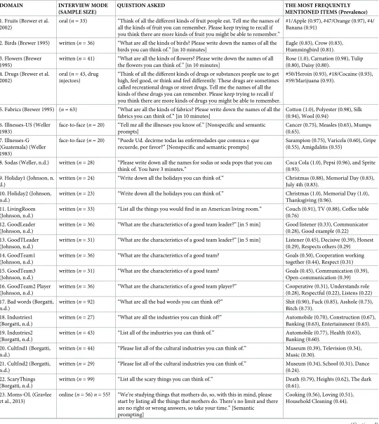
Some interviews were face to face, some were written responses, and some were adminis-tered on-line. Investigators varied in their use of prompts, using nonspecific (What other. . . are there?), semantic (repeating prior responses and then asking for others), and/or alphabetic prompts (going through the alphabet and asking for others). Brewer [29] and Gravlee et al. [30] specifically examined the effect of prompting on response productivity, although the Brewer et al. examples in these analyses contain results before extensive prompting and the Gravlee et al. examples contain results after prompting. The 28 examples, their topic, source, sample size, the question used in the original data collection, and the three most frequently mentioned items appear inTable 1. All data were collected and analyzed without personal identifying information.
Analysis
For each example, statistical models describe the pattern of obtaining new or unique items with incremental increases in sample size. Individual lists were first analyzed with Flame [31,32] to provide the list of unique items for each example and the Smith [14] and Sutrop [15] item salience scores. Duplicate items due to spelling, case errors, spacing, or variations were combined.
To help develop an interviewing stopping rule, a simple model was used to predict the unique number of items contributed by each additional respondent. Generalized linear models (GLM, log-linear models for count data) were used to predict the unique number of items added by each respondent (incrementing sample size), because number of unique items added by each respondent (count data) is approximately Poisson distributed. For each example, mod-els were fit with ordinary least squares linear regression, Poisson, and negative binomial proba-bility distributions. Respondents were assumed to be in random order, in the order in which they occurred in each dataset, although in some cases they were in the order they were inter-viewed. Goodness-of-fit was compared across the three models with minimized deviants (the Akaike Information Criterion, AIC) to find the best-fitting model [33]. Using the best-fitting model for each example, the point of saturation was estimated as the point where the expected number of new items was one or less. Sample size and domain size were estimated at the point of saturation, and total domain size was estimated for an infinite sample size from the model for each example as the limit of a geometric series (assuming a negative slope).
Because the GLM models above used only incremental sample size to predict the total num-ber of unique items (domain size) and ignored variation in the numnum-ber of items provided by each person and variation in item salience, an additional analysis was used to estimate domain size while accounting for subject and item heterogeneity. For that analysis, domain size was estimated with a capture-recapture estimation technique used for estimating the size of hidden populations. Domain size was estimated from the total number of items on individual lists and the number of matching items between pairs of lists with a log-linear analysis. For example, population size can be estimated from the responses of two people as the product of their num-ber of responses divided by the numnum-ber of matching items (assumed to be due to chance). If Person#1 named 15 illness terms and Person#2 named 31 terms and they matched on five ill-nesses, there would be 41 unique illness terms and the estimated total number of illness terms based on these two people would be (15 x 31) /5 = 93.
Table 1. The examples.
DOMAIN INTERVIEW MODE
(SAMPLE SIZE)
QUESTION ASKED THE MOST FREQUENTLY
MENTIONED ITEMS (Prevalence)
1. Fruits (Brewer et al. 2002)
oral (n= 33) “Think of all the different kinds of fruit people eat. Tell me the names of all the kinds of fruit you can remember. Please keep trying to recall if you think there are more kinds of fruit you might be able to remember.”
#1/Apple (0.97), #47/Orange (0.97), #4/ Banana (0.91)
2. Birds (Brewer 1995) written (n= 36) “What are all the kinds of birds? Please write down the names of all the birds you can think of.” [in 10 minutes]
Eagle (0.83), Crow (0.83), Hummingbird (0.81). 3. Flowers (Brewer
1995)
written (n= 41) “What are all the kinds of flowers? Please write down the names of all the flowers you can think of.” [in 10 minutes]
Rose (1.0), Carnation (0.98), Tulip (0.80), Daisy (0.80).
4. Drugs (Brewer et al. 2002)
oral (n= 43, drug injectors)
“Think of all the different kinds of drugs or substances people use to get high, feel good, or think and feel differently. These drugs are sometimes called recreational drugs or street drugs. Tell me the names of all the kinds of these drugs you can remember. Please keep trying to recall if you think there are more kinds of drugs you might be able to remember.
#50/Heroin (0.93), #18/Cocaine (0.93), #59/Marijuana (0.93).
5. Fabrics (Brewer 1995) (n= 63) “What are all the kinds of fabrics? Please write down the names of all the fabrics you can think of.” [in 10 minutes]
Cotton (1.0), Polyester (0.98), Silk (0.94), Wool (0.94)
6. Illnesses-US (Weller 1983)
face-to-face (n= 20) “Tell me all the illnesses you know of.” [Nonspecific and semantic prompts]
Cancer (0.75), Measles (0.65), Mumps (0.65).
7. Illnesses-G (Guatemala) (Weller 1983)
face-to-face (n= 20) “Puede Ud. decirme todas las enfermedades que conozca o que recuerde, por favor?” [Nonspecific and semantic prompts]
Sarampion (0.75), Varicela (0.60), Gripe (0.55), Amigdalitis (0.55)
8. Sodas (Weller, n.d.) written (n= 28) “Please write down all the names for sodas or soda pops that you can think of. You have 3 minutes.”
Coca Cola (1.0), Pepsi (0.96), and Sprite (0.93).
9. Holiday1 (Johnson, n. d.)
written (n= 24) “Write down all the holidays you can think of.” Christmas (0.88), Memorial Day (0.83), July 4th (0.83).
10. Holiday2 (Johnson, n.d.)
written (n= 23) “Write down all the holidays you can think of.” Christmas (1.0), Memorial Day (1.0), Thanksgiving (0.96).
11. LivingRoom (Johnson, n.d.)
written (n= 33) “List all the things you would find in an American living room.” Couch (0.91), TV (0.88), Coffee table (0.76)
12. GoodLeader (Johnson, n.d.)
written (n= 36) “What are the characteristics of a good team leader?” [in 5 min] Good listener (0.33), Communicator (0.28), Good example (0.22) 13. GoodTLeader
(Johnson, n.d.)
written (n= 31) “What are the characteristics of a good team leader?” [in 5 min] Listener (0.45), Decisive (0.39), Honest (0.29), Respects others (0.29) 14. GoodTeam1
(Johnson, n.d.)
written (n= 36) “What are the characteristics of a good team? Goals (0.50), Cooperation working together (0.44), Respect (0.31) 15. GoodTeam3
(Johnson, n.d.)
written (n= 31) “What are the characteristics of a good team? Goals (0.45), Communication (0.39), Open-communication (0.39) 16. GoodTeam2 Player
(Johnson, n.d.)
written (n= 36) “What are the characteristics of a good team player?” Cooperative (0.31), Understands role (0.28), Respectful (0.22), Listens (0.22) 17. Bad words (Borgatti,
n.d.)
written (n= 92) “What are all the bad words you can think of?” Shit (0.90), Fuck (0.85), Asshole (0.73), Bitch (0.73).
18. Industries1 (Borgatti, n.d.)
written (n= 27) “What are all the industries you can think of?” Automobile (0.70), Construction (0.67), Banking (0.63), Entertainment (0.63). 19. Industries2
(Borgatti, n.d.)
written (n= 43) “List all of the industries you can think of.” Automobile (0.77), Health (0.63), Banking (0.60).
20. CultInd1 (Borgatti, n.d.)
written (n= 44) “Please list all of the cultural industries you can think of.” Museum (0.39), Television (0.34), Music (0.30).
21. CultInd2 (Borgatti, n.d.)
written (n= 29) “Please list all of the cultural industries you can think of.” Museum (0.34), School (0.31), Dance (0.24).
22. ScaryThings (Borgatti, n.d.)
written (n= 99) “List all the scary things you can think of.” Death (0.79), Heights (0.62), The dark (0.61).
23. Moms-OL (Gravlee et al., 2013)
online (n= 56)n= 55? “We’re studying things that mothers do, so, with this in mind, please start by listing all the things that mothers do. There’s no limit and there are no right or wrong answers, so take your time.” [Semantic prompting]
Cooking (0.56), Loving (0.51), Household Cleaning (0.44).
not change between interviews (closed population) and models are fit with: (1) no variation across people or items (M0); (2) variation only across respondents (Mt); (3) variation only across items (Mh); and (4) variation due to an interaction between people and items (Mht). For each model, estimates were fit with binomial, Chao’s lower bound estimate, Poisson, Darroch log normal, and gamma distributions [35]. Variation among items (heterogeneity) is a test for a difference in the probabilities of item occurrence and, in this case, is equivalent to a test for a difference in item salience among the items. Due to the large number of combinations needed to estimate these models, Rcapture software estimates are provided for all four models only up to a sample of size 10. For larger sample sizes (all examples in this study had sample sizes of 20 or larger), only model 1 with no effects for people or items (the binomial model) and model 3 with item effects (item salience differences) were tested. Therefore, models were fit at size 10, to test all four models and then at the total available sample size.
Results
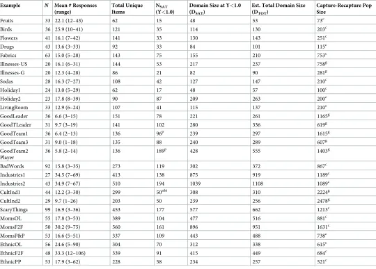
Descriptive information for the examples appears inTable 2. The first four columns list the name of the example, the sample size in the original study, the mean list length (with the range of the list length across respondents), and the total number of unique items obtained. For the Holiday1 example, interviews requested names of holidays (“Write down all the holidays you can think of”), there were 24 respondents, the average number of holidays listed per person (list length) was 13 (ranging from five to 29), and 62 unique holidays were obtained.
Predicting thematic saturation from sample size
The free-list counts showed a characteristicdescending curvewhere an initial person listed new themes and each additional person repeated some themes already reported and added new items, but fewer and fewer new items were added with incremental increases in sample size. All examples were fit using the GLM log-link and identity-link with normal, Poisson, and neg-ative binomial distributions. The negneg-ative binomial model resulted in a better fit than the Pois-son (or identity-link models) for most full-listing examples, providing the best fit to the downward sloping curve with a long tail. Of the 28 examples, only three were not best fit by negative binomial log-link models: the best-fitting model for two examples was the Poisson Table 1. (Continued)
DOMAIN INTERVIEW MODE
(SAMPLE SIZE)
QUESTION ASKED THE MOST FREQUENTLY
MENTIONED ITEMS (Prevalence)
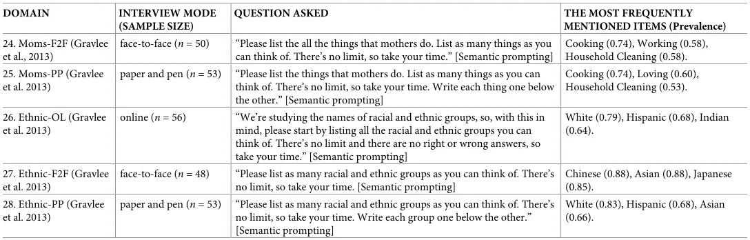
24. Moms-F2F (Gravlee et al., 2013)
face-to-face (n= 50) “Please list the all the things that mothers do. List as many things as you can think of. There’s no limit, so take your time.” [Semantic prompting]
Cooking (0.74), Working (0.58), Household Cleaning (0.58). 25. Moms-PP (Gravlee
et al. 2013)
paper and pen (n= 53) “Please list the things that mothers do. List as many things as you can think of. There’s no limit, so take your time. Write each thing one below the other.” [Semantic prompting]
Cooking (0.74), Loving (0.60), Household Cleaning (0.53).
26. Ethnic-OL (Gravlee et al. 2013)
online (n= 56) “We’re studying the names of racial and ethnic groups, so, with this in mind, please start by listing all the racial and ethnic groups you can think of. There’s no limit and there are no right or wrong answers, so take your time.” [Semantic prompting]
White (0.79), Hispanic (0.68), Indian (0.64).
27. Ethnic-F2F (Gravlee et al. 2013)
face-to-face (n= 48) “Please list as many racial and ethnic groups as you can think of. There’s no limit, so take your time. [Semantic prompting]
Chinese (0.88), Asian (0.88), Japanese (0.85).
28. Ethnic-PP (Gravlee et al. 2013)
paper and pen (n= 53) “Please list as many racial and ethnic groups as you can think of. There’s no limit, so take your time. Write each group one below the other.” [Semantic prompting]
White (0.83), Hispanic (0.68), Asian (0.66).
log-link model (GoodTeam1 and GoodTeam2Player) and one was best fit by the negative binomial identity-link model (CultInd1).
Sample size was a significant predictor of the number of new items for 21 of the 28 exam-ples. Seven examples did not result in a statistically significant fit (Illnesses-US, Holiday2, Industries1, Industries2, GoodTLeader, GoodTeam2Player, and GoodTeam3). The best-fitting model was used to predict the point of saturation and domain size for all 28 examples (S2
AppendixGLM Statistical Model Results for the 28 Examples).
Using the best-fitting GLM models we estimated the predicted sample size for reaching sat-uration. Saturation was defined as the point where less than one new item would be expected for each additional person interviewed. Using the models to solve for the sample size (X) when only one item was obtained per person (Y = 1) and rounding up to the nearest integer, pro-vided the point of saturation (Y1.0).Table 2, column five, reports the sample size where satu-ration was reached (NSAT). For Holiday1, one or fewer new items were obtained per person
Table 2. Estimated point of saturation and domain size.
Example N Mean # Responses (range)
Total Unique Items
NSAT
(Y<1.0)
Domain Size at Y<1.0 (DSAT)
Est. Total Domain Size (DTOT)
Capture-Recapture Pop Size
Fruits 33 22.1 (12–43) 62 15 48 53 73c
Birds 36 25.9 (10–41) 121 35 114 130 203c
Flowers 41 16.1 (7–42) 141 33 130 143 251c
Drugs 43 13.6 (3–33) 92 33 84 101 115c
Fabrics 63 15.0 (5–28) 143 75 155 210 753c
Illnesses-US 20 16.1 (6–31) 144 53 217 237 758g
Illnesses-G 20 12.3 (4–28) 86 21 82 90 281g
Sodas 28 16.3 (7–27) 108 42 127 147 210c
Holiday1 24 13.0 (5–29) 62 17 48 57 100c
Holiday2 23 17.8 (8–39) 90 87 209 263 200c
LivingRoom 33 12.9 (6–24) 107 41 115 137 210c
GoodLeader 36 6.6 (3–15) 151 78 221 261 1165g GoodTLeader 31 9.7 (3–19) 141 102 280 336 619g
GoodTeam1 36 6.4 (2–13) 136 96p 239 297 1615g
GoodTeam3 31 9.0 (1–18) 135 88 240 289 607g
GoodTeam2 Player
36 5.8 (2–14) 136 189p 428 555 1403g
BadWords 92 15.8 (3–35) 273 119 302 372 867c Industries1 27 34.5 (7–69) 413 138 875 919 1189c
Industries2 43 34.9 (7–67) 510 194 1039 1108 1089c
CultInd1 44 12.2 (3–30) 299 50nbi 308 310 2224g
CultInd2 29 9.7 (1–26) 203 50 239 256 2478g
ScaryThings 99 16.9 (3–36) 453 177 577 662 1213c
MomsOL 55 17.8 (3–53) 389 104 477 516 881c
MomsF2F 50 30.2 (9–75) 560 161 896 951 1631c
MomsP&P 53 16.6 (5–51) 337 109 443 488 738c
EthnicOL 56 24.6 (5–90) 304 70 312 338 615c
EthnicF2F 48 33.3 (12–106) 339 91 415 449 684c
EthnicPP 53 17.9 (3–62) 228 58 234 257 521c
nbi = Negative binomial-identity, p = Poisson-log ; c = Chao’s Lower bound; g = gamma
when X = 16.98. Rounding up to the next integer provides the saturation point (NSAT= 17).
For the Fruit domain, saturation occurred at a sample size of 15.
Saturation was reached at sample sizes of 15–194, with a median sample size of 75. Only five examples (Holiday1, Fruits, Birds, Flowers, and Drugs) reached saturation within the orig-inal study sample size and most examples did not reach saturation even after four or five dozen interviews. A more liberal definition of saturation, defined as the point where less than two new items would be expected for each additional person (solving for Y2), resulted in a median sample size for reaching saturation of 50 (range 10–146).
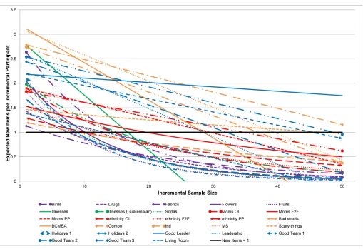
Some domains were well bounded and were elicited with small sample sizes. Some were not. In fact, most of the distributions exhibited a very long tail–where many items were men-tioned by only one or two people.Fig 1shows the predicted curves for all examples for sample sizes of 1 to 50. Saturation is the point where the descending curve crosses Y = 1 (or Y = 2). Although the expected number of unique ideas or themes obtained for successive respondents tends to decrease as the sample size increases, this occurs rapidly in some domains and slowly or not at all in other domains. Fruits, Holiday1, and Illness-G are domains with the three bot-tom-most curves and the steepest descent, indicating that saturation was reached rapidly and with small sample sizes. The three top-most curves are the Moms-F2F, Industries1, and Indus-tries2 domains, which reached saturation at very large sample sizes or essentially did not reach saturation.
Fig 1. The number of unique items provided with increasing sample size.
Estimating domain size
Because saturation appeared to be related to domain size and some investigators state that a percentage of the domain might be a better standard [25], domain size was also estimated. First, total domain size was estimated with the GLM models obtained above. Domain size was estimated at the point of saturation by cumulatively summing the number of items obtained for sample sizesn= 1,n= 2,n= 3,. . .to NSAT. For the Holiday1 sample, summing the number
of predicted unique items for sample sizesn= 1 ton= 17 should yield 51 items (Table 2, Domain Size at Saturation, DSAT). Thus, the model predicted that approximately 51 holidays
would be obtained by the time saturation was reached.
The total domain size was estimated using a geometric series, summing the estimated num-ber of unique items obtained cumulatively across people in an infinitely large sample. For the Holiday1 domain, the total domain size was estimated as 56 (seeTable 2, Total Domain Size DTOT). So for the Holiday1 domain, although the total domain size was estimated to be 57, the
model predicted that saturation occurred when the sample size reached 17, and at that point 51 holidays should be retrieved. Model predictions were close to the empirical data, as 62 holi-days were obtained with a sample of 24.
Larger sample sizes were needed to reach saturation in larger domains; the largest domains were MomsF2F, Industries1, and Industries2 each estimated to have about 1,000 items and more than 100 interviews needed to approach saturation. Saturation (Y1) tended to occur at about 90% of the total domain size. For Fruits, the domain size at saturation was 51 and the total domain size was estimated at 53 (51/53 = 96%) and for MomsF2F, domain size at satura-tion was 904 and total domain size was 951 (95%).
Second, total domain size was estimated using a capture-recapture log-linear model with a parameter for item heterogeneity [35,36]. A descending, concave curve is diagnostic of item heterogeneity and was present in almost all of the examples. The estimated population sizes using R-Capture appear in the last column ofTable 2. When the gamma distribution provided the best fit to the response data, the domain size increased by an order of magnitude as did the standard error on that estimate. When responses fit a gamma distribution, the domain may be extremely large and may not readily reach saturation.
Inclusion of the pattern of matching items across people with a parameter for item hetero-geneity (overlap in items between people due to salience) resulted in larger population size estimates than those above without heterogeneity. Estimation from the first two respondents was not helpful and provided estimates much lower than those from any of the other methods. The simple model without subject or item effects (the binomial model) did not fit any of the examples. Estimation from the first 10 respondents in each example suggested that more varia-tion was due to item heterogeneity than to item and subject heterogeneity, so we report only the estimated domain size with the complete samples accounting for item heterogeneity in salience.
Overall, the capture–recapture estimates incorporating the effect of salience were larger than the GLM results above without a parameter for salience. For Fruits, the total domain size was estimated as 45 from the first two people; as 88 (gamma distribution estimate) from the first 10 people with item heterogeneity and as 67 (Chao lower bound estimate) with item and subject heterogeneity; and using the total sample (n= 33) the binomial model (without any heterogeneity parameters) estimated the domain size as 62 (but did not fit the data) and with item heterogeneity the domain size was estimated as 73 (the best-fitting model used the Chao lower bound estimate). Thus, the total domain size for Fruits estimated with a simple GLM model was 53 and with a capture–recapture model (including item heterogeneity) was 73
simple GLM model and 100 with capture-recapture model. Domain size estimates suggest that even the simplest domains can be large and that inclusion of item heterogeneity increases domain size estimates.
Saturation and the number of responses per person
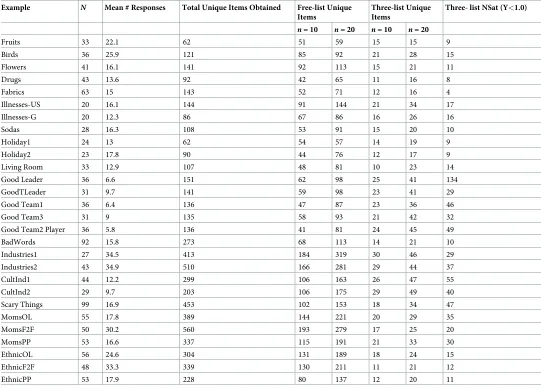
The original examples used an exhaustive listing of responses to obtain about a half dozen (GoodLeader and GoodTeam2Player) to almost three dozen responses per person (Industries1 and Industries2). A question is whether saturation and the number of unique ideas obtained might be affected by the number of responses per person. Since open-ended questions may obtain only a few responses, we limited the responses to a maximum of three per person, trun-cating lists to see the effect on the number of items obtained at different sample sizes and the point of saturation.
When more information (a greater number of responses) was collected per person, more unique items were obtained even at smaller sample sizes (Table 3). The amount of information retrieved per sample can be conceived of in terms of bits of information per sample and is roughly the average number of responses per person times the sample size so that, with all
Table 3. Comparison of number of unique items obtained with full free lists and with three or fewer responses.
Example N Mean # Responses Total Unique Items Obtained Free-list Unique Items
Three-list Unique Items
Three- list NSat (Y<1.0)
n= 10 n= 20 n= 10 n= 20
Fruits 33 22.1 62 51 59 15 15 9
Birds 36 25.9 121 85 92 21 28 15
Flowers 41 16.1 141 92 113 15 21 11
Drugs 43 13.6 92 42 65 11 16 8
Fabrics 63 15 143 52 71 12 16 4
Illnesses-US 20 16.1 144 91 144 21 34 17
Illnesses-G 20 12.3 86 67 86 16 26 16
Sodas 28 16.3 108 53 91 15 20 10
Holiday1 24 13 62 54 57 14 19 9
Holiday2 23 17.8 90 44 76 12 17 9
Living Room 33 12.9 107 48 81 10 23 14
Good Leader 36 6.6 151 62 98 25 41 134
GoodTLeader 31 9.7 141 59 98 23 41 29
Good Team1 36 6.4 136 47 87 23 36 46
Good Team3 31 9 135 58 93 21 42 32
Good Team2 Player 36 5.8 136 41 81 24 45 49
BadWords 92 15.8 273 68 113 14 21 10
Industries1 27 34.5 413 184 319 30 46 29
Industries2 43 34.9 510 166 281 29 44 37
CultInd1 44 12.2 299 106 163 26 47 55
CultInd2 29 9.7 203 106 175 29 49 40
Scary Things 99 16.9 453 102 153 18 34 47
MomsOL 55 17.8 389 144 221 20 29 35
MomsF2F 50 30.2 560 193 279 17 25 20
MomsPP 53 16.6 337 115 191 21 33 30
EthnicOL 56 24.6 304 131 189 18 24 15
EthnicF2F 48 33.3 339 130 211 11 21 12
EthnicPP 53 17.9 228 80 137 12 20 11
other things being equal, larger sample sizes with less probing should approach the same amount of information obtained with smaller samples and more probing. So, for a given sam-ple size, a study with six responses per person should obtain twice as much information as a study with three responses per person. In the GoodLeader, GoodTeam1, and GoodTeam2-Player examples, the average list length was approximately six and when the sample size was 10 (6 x 10 = 60 bits of information), approximately twice as many items were obtained as when lists were truncated to three responses (3 x 10 = 30 bits of information).
Increasing the sample size proportionately increases the amount of information, but not always. For Scary Things, 5.6 bits more information were collected per person with full listing (16.9 average list length) than with three or fewer responses per person (3.0 list length); and the number of items obtained in a sample size of 10 with full listing (102) was roughly 5.6 times greater than that obtained with three responses per person (18 items). However, at a sample size of 20 the number of unique items with free lists was only 4.5 times larger (153) than the number obtained with three responses per person (34).Across examples,interviews that obtained more information per person were more productive and obtained more unique items overall even with smaller sample sizes than did interviews with only three responses per person.
Using the same definition of saturation (the point where less than one new item would be expected for each additional person interviewed), less information per person resulted in reaching saturation at muchsmallersample sizes.Fig 2shows the predicted curves for all examples when the number of responses per person is three (or fewer). The Holiday examples reached saturation (fewer than one new item per person) with a sample size of 17 (Holiday1) with 13.0 average responses per person and 87 (Holiday2) with 17.8 average responses
(Table 2), but reached saturation with a sample size of only 9 (Holiday 1 and Holiday2) when
there were a maximum of three responses per person (Table 3, last column). With three or fewer responses per person, the median sample size for reaching saturation was 16 (range: 4–134). Thus, fewer responses per person resulted in reaching saturation at smaller sample sizes and resulted in fewer domain items.
Salience and sample size
Saturation did not seem to be a useful guide for determining a sample size stopping point, because it was sensitive both to domain size and the number of responses per person. Since a main goal of open-ended interviews is to obtain the most important ideas and themes, it seemed reasonable to consider item salience as an alternative guide to assist with determining sample size adequacy. Here, the question would be: Whether or not complete saturation is achieved, are the most salient ideas and themes captured in small samples?
To test whether the most salient ideas and themes were captured in smaller samples or with limited probing, we used the sample proportions to estimate item salience and compared the set of most salient items across sample sizes and across more and less probing. Specifically, we defined a set of salient items for each example as those mentioned by 20% or more in the sam-ple of size 20 (because all examsam-ples had at least 20) with full-listing (because domains were more detailed). We compared the set of salient items with the set of items obtained at smaller sample sizes and with fewer responses per person.
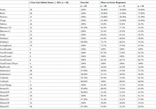
The set size for salient items (prevalence20%) was not related to overall domain size, but was an independent characteristic of each domain and whether there were core or prototypical items with higher salience. Most domains had about two dozen items mentioned by 20% or more of the original listing sample (n= 20), but some domains had only a half dozen or fewer items (GoodLeader, GoodTeam2Player, GoodTeam3). With full listing, 26 of 28 examples cap-tured more than 95% of the salient ideas in the first 10 interviews: 18 examples capcap-tured 100%, eight examples captured 95–99%, one example captured 91%, and one captured 80% (Table 4). With a maximum of three responses per person, about two-thirds of the salient items (68%) were captured with 20 interviews and about half of the items (53%) were captured in the first 10 interviews. With a sample size of 20, a greater number of responses per person resulted in approximately 50% more items than with three responses per person. Extensive probing resulted in a greater capture of salient items even with smaller sample sizes.
Fig 2. The number of unique items provided with increasing sample size when there are three or fewer responses per person.
Summary and discussion
The strict notion of complete saturation as the point where few or no new ideas are observed is not a useful concept to guide sample size decisions, because it is sensitive to domain size and the amount of information contributed by each respondent. Larger sample sizes are necessary to reach saturation for large domains and it is difficult to know, when starting a study, just how large the domain or set of ideas will be. Also, when respondents only provide a few responses or codes per person, saturation may be reached quickly. So, if complete thematic sat-uration is observed, it is difficult to know whether the domain is small or whether the inter-viewer did only minimal probing.
Rather than attempting to reach complete saturation with an incremental sampling plan, a more productive focus might be on gaining more depth with probing and seeking the most salient ideas. Rarely do we needallthe ideas and themes, rather we tend to be looking for important or salient ideas. A greater number of responses per person resulted in the capture of a greater number of salient items. With exhaustive listing, the first 10 interviews obtained 95% of the salient ideas (defined here as item prevalence of 0.20 or more), while only 53% of those ideas were obtained in 10 interviews with three or fewer responses per person.
Table 4. Capture of salient items with full free list and with three or fewer responses.
# Free-List Salient Items (20%, n = 20) Free-list Three or Fewer Responses
n= 10 n= 20 n= 15 n= 10
Fruits 38 100% 36.80% 36.80% 36.80%
Birds 46 100% 50.00% 47.80% 37.00%
Flowers 31 100% 54.80% 48.40% 41.90%
Drugs 21 100% 61.90% 42.90% 42.90%
Fabrics 26 100% 53.8% 53.8% 42.3%
Illnesses-US 22 95.50% 81.8% 77.3% 54.5%
Illnesses-G 21 100% 52.4% 47.6% 47.6%
Sodas 23 100% 69.6% 65.2% 56.5%
Holiday1 20 100% 65.0% 60.0% 50.0%
Holiday2 22 90.90% 72.7% 68.2% 54.5%
LivingRoom 19 100% 73.7% 57.9% 47.4%
GoodLeader 4 100% 100% 100% 100%
GoodTLeader 8 100% 87.5% 75.0% 62.5%
GoodTeam1 6 100% 100% 100% 83.3%
GoodTeam3 6 100% 83.3% 66.7% 66.7%
GoodTeam2 Player 4 100% 100% 100% 100%
BadWords 25 100% 56.0% 56.0% 44.0%
Industries1 48 97.90% 50.0% 47.9% 37.5%
Industries2 49 98.00% 53.1% 49.0% 38.8%
CultInd1 23 95.70% 87.0% 73.9% 65.2%
CultInd2 5 80.00% 100% 80.0% 60.0%
ScaryThings 11 100% 81.8% 72.7% 63.6%
MomsOL 20 95.00% 80.0% 70.0% 65.0%
MomsF2F 31 96.80% 51.6% 51.6% 41.9%
MomsPP 18 100% 83.3% 72.2% 61.1%
EthnicOL 37 97.30% 51.4% 43.2% 37.8%
EthnicF2F 52 100% 30.8% 28.8% 19.2%
EthnicPP 40 97.50% 35.0% 32.5% 20.0%
We used a simple statistical model to predict the number of new items added by each addi-tional person and found that complete saturation was not a helpful concept for free-lists, as the median sample size was 75 to get fewer than one new idea per person. It is important to note that we assumed that interviews were in a random order or were in the order that the inter-views were conducted and were not reordered to any kind of optimum. The reordering of respondents to maximally fit a saturation curve may make it appear that saturation has been reached at a smaller sample size [31].
Most of the examples examined in this study needed sample sizes larger than most qualitative researchers use to reach saturation. Mason’s [6] review of 298 PhD dissertations in the United Kingdom, all based on qualitative data, found a mean sample size of 27 (range 1–95). Here, few of the examples reached saturation with less than four dozen interviews. Even with large sample sizes, some domains may continue to add new items. For very large domains, an incremental sampling strategy may lead to dozens and dozens of interviews and still not reach complete sat-uration. The problem is that most domains have very long tails in the distribution of observed items, with many items mentioned by only one or two people. A more liberal definition of com-plete saturation (allowing up to two new items per person) allowed for saturation to occur at smaller sample sizes, but saturation still did not occur until a median sample size of 50.
In the examples we studied, most domains were large and domain size affected when satu-ration occurred. Unfortunately, there did not seem to be a good or simple way at the outset to tell if a domain would be large or small. Most domains were much larger than expected, even on simple topics. Domain size varied by substantive content, sample, and degree of heteroge-neity in salience. Domain size and saturation were sample dependent, as the holiday examples showed. Also, domain size estimates did not mean that there are only 73 fruits, rather the pat-tern of naming fruits–for this particular sample–indicated a set size of 73.
It was impossible to know, when starting, if a topic or domain was small and would require 15 interviews to reach saturation or if the domain was large and would require more than 100 interviews to reach saturation. Although eight of the examples had sample sizes of 50–99, sam-ple sizes in qualitative studies are rarely that large. Estimates of domain size were even larger when models incorporated item heterogeneity (salience). The Fruit example had an estimated domain size of 53 without item heterogeneity, but 73 with item heterogeneity. The estimated size of the Fabric domain increased from 210 to 753 when item heterogeneity was included.
The number of responses per person affected both saturation and the number of obtained items. A greater number of responses per person resulted in a greater yield of domain items. The bits of information obtained in a sample can be approximated by the product of the aver-age number of responses per person (list length) and the number of people in a sample. How-ever, doubling the sample size did not necessarily double the unique items obtained because of item salience and sampling variability. When only a few items are obtained from each person, only the most salient items tend to be provided by each person and fewer items are obtained overall.
Brewer [29] explored the effect of probing or prompting on interview yield. Brewer exam-ined the use of a few simple prompts: simply asking for more responses, providing alphabetical cues, or repeating the last response(s) and asking again for more information. Semantic cue-ing, repeating prior responses and asking for more information, increased the yield by approx-imately 50%. The results here indicated a similar pattern. When more information was elicited per person, about 50% more domain items were retrieved than when people provided a maxi-mum of three responses.
of the domain items. Unfortunately, different degrees of salience among items may cause strong effects for respondents to repeat similar ideas–the most salient ideas–without elaborat-ing on less salient or less prevalent ideas, resultelaborat-ing in a set of only the ideas with the very high-est salience.If an investigator wishes to obtain most of the ideas that are relevant in a domain,a small sample with extensive probing (listing) will prove much more productive than a large sample with casual or no probing.
Recently, Galvin [21] and Fugard and Potts [22] framed sample size estimation for qualita-tive interviewing in terms of binomial probabilities. However, results for the 28 examples with multiple responses per person suggest that this may not be appropriate because of the interde-pendencies among items due to salience. The capture–recapture analysis indicated that none of the 28 examples fit the binomial distribution. Framing the sample size problem in terms that a specific idea or theme will or will not appear in a set of interviews may facilitate thinking about sample size, but such estimates may be misleading.
If a binomial distribution is assumed, sample size can be estimated from the prevalence of an idea in the population, from how confident you want to be in obtaining these ideas, and from how many times you would like these ideas to minimally appear across participants in your interviews. A binomial estimate assumes independence (no difference in salience across items) and predicts that if an idea or theme actually occurs in 20% of the population, there is a 90% or higher likelihood of obtaining those themesat least oncein 11 interviews and a 95% likelihood in 14 interviews. In contrast, our results indicated that the heterogeneity in salience across items causes these estimates to underestimate the necessary sample size as items with 20% prevalence were captured in 10 interviews in only 64% of the samples with full listing and in only 4% (one) of samples with three or fewer responses.
Lowe et al. [25] also found that items were not independent and that binomial estimates sig-nificantly underestimated sample size. They proposed sample size estimation from the desired proportion of items at a given average prevalence. Their formula predicts that 36 interviews would be necessary to capture 90% of items with an average prevalence of 0.20, regardless of degree of heterogeneity in salience, domain size, or amount of information provided per respondent. Although they included a parameter for non-independence, their model does not seem to be accurate for cases with limited responses or for large domains.
Conclusions
In general,probing and prompting during an interview seems to matter more than the number of interviews. Thematic saturation may be an illusion and may result from a failure to use in-depth probing during the interview. A small sample (n= 10) can collect some of the most salient ideas, but a small sample with extensive probing can collect most of the salient ideas. A larger sample (n= 20) is more sensitive and can collect more prevalent and more salient ideas, as well as less prevalent ideas, especially with probing. Some domains, however, may not have items with high prevalence. Several of the domains examined had only a half dozen or fewer items with prevalence of 20% or more. The direct link between salience and population preva-lence offers a rationale for sample size and facilitates study planning. If the goal is to get a few widely held ideas, a small sample size will suffice. If the goal is to explore a larger range of ideas, a larger sample size or extensive probing is needed. Sample sizes of one to two dozen interviews should be sufficient with exhaustive probing (listing interviews), especially in a coherent domain. Empirically observed stabilization of item salience may indicate an adequate sample size.
questions in large surveys. Open-ended survey questions are inefficient and result in thin or sparse data with few responses per person because of a lack of prompting. Tran et al. [24] reported item prevalence of 0.025 in answers in a large Internet survey suggesting few responses per person. In contrast, we used an item prevalence of 0.20 and higher to identify the most salient items in each domain and the highest prevalence in each domain ranged from 0.30 to 0.80 (Table 1). Inefficiency in open-ended survey questions is likely due to the dual pur-pose of the questions: They try to define the range of possible answersandget the respondent’s answer. A better approach might be to precede survey development with a dozen free-listing interviews to get the range of possible responses and then use that content to design structured survey questions.
Another avenue for investigation is how our findings onthematic saturationcompare to theoretical saturationin grounded theory studies [2,38,39]. Grounded theory studies rely on theoretical sampling–-an iterative procedure in which a single interview is coded for themes; the next respondent is selected to discover new themes and relationships between themes; and so on, until no more relevant themes or inter-relationships are discovered and a theory is built to explain the facts/themes of the case under study. In contrast this study examined thematic saturation, the simple accumulation of ideas and themes, and found that saturation in salience was more attainable–-perhaps more important–than thematic saturation.
Supporting information
S1 Appendix. The original data for the 28 examples. (XLSX)
S2 Appendix. GLM statistical model results for the 28 examples. (DOCX)
Acknowledgments
We would like to thank Devon Brewer and Kristofer Jennings for providing feedback on an earlier version of this manuscript. We would also like to thank Devon Brewer for providing data from his studies on free-lists.
Author Contributions
Conceptualization: Susan C. Weller, H. Russell Bernard, Jeffrey C. Johnson.
Data curation: Ben Vickers.
Formal analysis: Ben Vickers.
Investigation: Ben Vickers.
Methodology: Susan C. Weller, Ben Vickers, H. Russell Bernard, Alyssa M. Blackburn, Ste-phen Borgatti, Clarence C. Gravlee, Jeffrey C. Johnson.
Project administration: Susan C. Weller.
Resources: Susan C. Weller, Stephen Borgatti, Clarence C. Gravlee, Jeffrey C. Johnson.
Supervision: Susan C. Weller.
Writing – original draft: Susan C. Weller.
References
1. Glaser BG. The constant comparative method of qualitative analysis. Soc Probl. 1965; 12: 436−445. 2. Glaser BG, Strauss AL. The discovery of grounded theory: Strategies for qualitative research. New
Brunswick, NJ: Aldine, 1967.
3. Lincoln YS, Guba EG. Naturalistic inquiry. Beverly Hills, CA: Sage, 1985.
4. Morse JM. Strategies for sampling. In: Morse JM, editor, Qualitative Nursing Research: A Contempo-rary Dialogue. Rockville, MD: Aspen Press, 1989, pp. 117–131.
5. Sandelowski M. Sample size in qualitative research. Res Nurs Health. 1995; 18:179−183. PMID:
7899572
6. Mason M. Sample size and saturation in PhD studies using qualitative interviews. Forum: Qualitative Social Research 2010; 11.http://nbn-resolving.de/urn:nbn:de:0114-fqs100387(accessed December 26, 2017).
7. Thompson EC, Juan Z. Comparative cultural salience: measures using free-list data. Field Methods. 2006; 18: 398–412.
8. Romney A, D’Andrade R. Cognitive aspects of English kin terms. Am Anthro. 1964; 66: 146–170. 9. Bousfield WA, Barclay WD. The relationship between order and frequency of occurrence of restricted
associative responses. J Exp Psych. 1950; 40: 643–647.
10. Geeraerts D. Theories of lexical semantics. Oxford University Press, 2010. 11. Hajibayova L. Basic-Level Categories a Review. J of Info Sci. 2013; 1–12.
12. Berlin Brent. Ethnobiological classification. In: Rosch E, Lloyd BB, eds. Cognition and Categorization. Hillsdale, NJ: Erlbaum. 1978, pp 9–26.
13. Smith JJ, Furbee L, Maynard K, Quick S, Ross L. Salience counts: A domain analysis of English color terms. J Linguistic Anthro. 1995; 5(2): 203–216.
14. Smith JJ, Borgatti SP. Salience counts-and so does accuracy: Correcting and updating a measure for free-list-item salience. J Linguistic Anthro. 1997; 7: 208–209.
15. Sutrop U. List task and a cognitive salience index. Field Methods. 2001; 13(3): 263–276.
16. Robbins MC, Nolan JM, Chen D. An improved measure of cognitive salience in free listing tasks: a Mar-shallese example. Field Methods. 2017; 29:395−9:395.
17. Guest G, Bunce A, Johnson L. How many interviews are enough? An experiment with data saturation and variability. Field Methods. 2006; 18: 59–82.
18. Coenen M, Stamm TA, Stucki G, Cieza A. Individual interviews and focus groups in patients with rheu-matoid arthritis: A comparison of two qualitative methods. Quality of Life Research. 2012; 21:359–70.
https://doi.org/10.1007/s11136-011-9943-2PMID:21706128
19. Francis JJ, Johnston M, Robertson C, Glidewell L, Entwistle V, Eccles MP, et al. What is an adequate sample size? Operationalising data saturation for theory-based interview studies. Psychol Health. 2010; 25:1229–45.https://doi.org/10.1080/08870440903194015PMID:20204937
20. Hagaman A K, Wutich A. How many interviews are enough to identify metathemes in multisited and cross-cultural research? Another perspective on Guest, Bunce, and Johnson’s (2006) landmark study. Field Methods. 2017; 29:23−41.
21. Galvin R. How many interviews are enough? Do qualitative interviews in building energy consumption research produce reliable knowledge? J of Building Engineering, 2015; 1: 2–12.
22. Fugard AJ, Potts HW. Supporting thinking on sample sizes for thematic analyses: a quantitative tool. Int J Soc Res Methodol. 2015; 18: 669–684.
23. Bernard HR, Killworth PD. Sampling in time allocation research. Ethnology. 1993; 32:207–15. 24. Tran VT, Porcher R, Tran VC, Ravaud P. Predicting data saturation in qualitative surveys with
mathe-matical models from ecological research. J Clin Epi. 2017; Feb; 82:71–78.e2.https://doi.org/10.1016/j. jclinepi.2016.10.001Epub 2016 Oct 24. PMID:27789316
25. Lowe A, Norris AC, Farris AJ, Babbage DR. Quantifying thematic saturation in qualitative data analysis. Field Methods. 2018; 30 (in press, online first:http://journals.sagepub.com/doi/full/10.1177/
1525822X17749386).
26. Van Rijnsoever FJ. (I Can’t Get No) Saturation: A simulation and guidelines for sample sizes in qualita-tive research. PLoS ONE. 2017; 12: e0181689.https://doi.org/10.1371/journal.pone.0181689PMID:
28746358
28. Brewer DD. Cognitive indicators of knowledge in semantic domains. J of Quant Anthro. 1995; 5: 107– 128.
29. Brewer DD. Supplementary interviewing techniques to maximize output in free listing tasks. Field Meth-ods. 2002; 14: 108–118.
30. Gravlee CC, Bernard HR, Maxwell CR, Jacobsohn A. Mode effects in free-list elicitation: comparing oral, written, and web-based data collection. Soc Sci Comput Rev. 2013; 31: 119–132.
31. Pennec F, Wencelius J, Garine E, Bohbot H. Flame v1.2–Free-list analysis under Microsoft Excel (Soft-ware and English User Guide), 2014. Available from:https://www.researchgate.net/publication/ 261704624_Flame_v12_-_Free-List_Analysis_Under_Microsoft_Excel_Software_and_English_User_ Guide(10/19/17)
32. Borgatti SP. Software review: FLAME (Version 1.1). Field Methods. 2015; 27:199–205.
33. SAS Institute Inc. GENMOD. SAS/STAT®13.1 User’s Guide. Cary, NC: SAS Institute Inc., 2013. 34. Bishop Y, Feinberg S, Holland P. Discrete multivariate statistics: Theory and practice, MIT Press,
Cambridge, 1975.
35. Baillargeon S, Rivest LP. Rcapture: loglinear models for capture-recapture in R. J Statistical Software. 2007; 19: 1–31.
36. Rivest LP, Baillargeon S: Package ‘Rcapture’ Loglinear models for capture-recapture experiments, in CRAN, R, Documentation Feb 19, 2015.
37. Weller SC, Romney AK. Systematic data collection (Vol. 10). Sage, 1988.
38. Morse M. Theoretical saturation. In Lewis-Beck MS, Bryman A, Liao TF, editors. The Sage encyclope-dia of social science research methods. Thousand Oaks, CA: Sage, 2004, p1123. Available from
http://sk.sagepub.com/reference/download/socialscience/n1011.pdf