ASREML user guide release 3.0

(1)

Patron: Her Majesty The Queen Rothamsted Research Harpenden, Herts, AL5 2JQ

Telephone: +44 (0)1582 763133 Web: http://www.rothamsted.ac.uk/

Rothamsted Research is a Company Limited by Guarantee Registered Office: as above. Registered in England No. 2393175. Registered Charity No. 802038. VAT No. 197 4201 51. Founded in 1843 by John Bennet Lawes.

Rothamsted Repository Download

D1 - Technical reports: non-confidential

Gilmour, A. R., Gogel, B. J., Cullis, B. R. and Thompson, R. 2009.

ASREML user guide release 3.0. VSN International, Hemel Hempstead.

The publisher's version can be accessed at:

• https://www.vsni.co.uk/downloads/asreml/release3/UserGuide.pdf

The output can be accessed at:

https://repository.rothamsted.ac.uk/item/8w146

.

© VSN International, Hemel Hempstead.

(2)

ASReml

User Guide

Release 3.0

2009

(3)

ASReml User Guide Release 3.0

ASReml is a statistical package that fits linear mixed models using Residual Maximum Likelihood (REML). It is a joint venture between the Biometrics Pro-gram of NSW Department of Primary Industries and the Biomathematics Unit of Rothamsted Research. Statisticians in Britain and Australia have collaborated in its development.

Main authors:

A. R. Gilmour, B. J. Gogel, B. R. Cullis and R. Thompson

Other contributors:

D. Butler, M. Cherry, D. Collins, G. Dutkowski, S. A. Harding, K. Haskard, A. Kelly, S. G. Nielsen, A. Smith, A. P. Verbyla, S. J. Welham and I. M. S. White.

Author email addresses

[email protected] [email protected] [email protected] [email protected]

Copyright Notice

(4)

Published by:

VSN International Ltd, 5 The Waterhouse, Waterhouse Street, Hemel Hempstead, HP1 1ES, UK E-mail: [email protected] Website: http://www.vsni.co.uk/

The correct bibliographical reference for this document is:

(5)

Preface

ASRemlis a statistical package that fits linear mixed models using Residual Max-imum Likelihood (REML). It has been under development since 1993 and is a joint venture between the Biometrics Program of NSW Department of Primary Industries and the Biomathematics and Bioinformatics Division (previously the Statistics Department) of Rothamsted Research. Release 2 of ASReml was dis-tributed in 2006. This guide relates to Release 3 first disdis-tributed in 2008. Changes in this version are indicated by the wordASReml3in the margin. Features added ASReml3

in Release 2 have ASReml2in the margin. Other significant changes to the text ASReml2

are indicated byRevised in the margin. A separate document,ASReml 3 Update, Revised 08

is available to highlight the changes from Release 2.00.

Linear mixed effects models provide a rich and flexible tool for the analysis of many data sets commonly arising in the agricultural, biological, medical and en-vironmental sciences. Typical applications include the analysis of (un)balanced longitudinal data, repeated measures analysis, the analysis of (un)balanced de-signed experiments, the analysis of multi-environment trials, the analysis of both univariate and multivariate animal breeding and genetics data and the analysis of regular or irregular spatial data.

ASRemlprovides a stable platform for delivering well established procedures while also delivering current research in the application of linear mixed models. The strength of ASReml is the use of the Average Information (AI) algorithm and sparse matrix methods for fitting the linear mixed model. This enables it to analyse large and complex data sets quite efficiently.

One of the strengths of ASRemlis the wide range of variance models for the ran-dom effects in the linear mixed model that are available. There is a potential cost for this wide choice. Users should be aware of the dangers of either overfitting or attempting to fit inappropriate variance models to small or highly unbalanced data sets. We stress the importance of using data-driven diagnostics and encour-age the user to read the examples chapter, in which we have attempted to not only present the syntax of ASReml in the context of real analyses but also to

(6)

Preface ii

indicate some of the modelling approaches we have found useful.

There are several interfaces to the core functionality of ASReml. The program Revised 08

name ASReml relates to the primary program. ASReml-W refers to the user interface program developed by VSN and distributed with ASReml. ASReml-R

refers to the S language interface to a DLL of the core ASRemlroutines. Genstat

uses the same core routines for its REML directive. Both of these have good data manipulation and graphical facilities.

The focus in developing ASReml has been on the core engine and it is freely acknowledged that its user interface is not to the level of these other packages. Nevertheless, as the developers interface, it is functional, it gives access to every-thing that the core can do and is especially suited to batch processing and running of large models without the overheads of other systems. Feedback from users is welcome and attempts will be made to rectify identified problems in ASReml.

The guide has 15 chapters. Chapter 1 introducesASRemland describes the con-ventions used in this guide. Chapter 2 outlines some basic theory while Chapter 3 presents an overview of the syntax ofASRemlthrough a simple example. Data file preparation is described in Chapter 4 and Chapter 5 describes how to input data intoASReml. Chapters 6 and 7 are key chapters which present the syntax for specifying the linear model and the variance models for the random effects in the linear mixed model. Chapters 8 and 9 describe special commands for multivari-ate and genetic analyses respectively. Chapter 10 deals with prediction of linear functions of fixed and random effects in the linear mixed model and Chapter 13 presents the syntax for forming functions of variance components. Chapter 11 demonstrates running an ASReml job features available and Chapter 14 gives a detailed explanation of the output files. Chapter 15 gives an overview of the error messages generated inASRemland some guidance as to their probable cause. The guide concludes with the most extensive chapter which presents the examples.

Briefly, the improvements in Release 2 include more robust variance parameter updating so that ’Convergence Failure’ is less likely, extensions to the syntax, inclusion of the Mat´ern correlation model, ability to plot predicted values, im-provements for testing fixed effects, imim-provements to the handling of pedigrees and some increases in computational speed.

Release 3 contains some extensions to data handling (merging files), pedigree pro-ASReml3

cessing, model specification, theshold models, prediction and examining residuals.

(7)

Preface iii

http://www.vsni.co.uk/products/asreml as well as in the examples direc-tory of the distribution CD-ROM. They remain the property of the authors or of the original source but may be freely distributed provided the source is acknowl-edged. The authors would appreciate feedback and suggestions for improvements to the program and this guide.

Proceeds from the licensing of ASReml are used to support continued develop-ment to impledevelop-ment new developdevelop-ments in the application of linear mixed models. The developmental version is available to supported licensees via a website upon request to VSN. Most users will not need to access the developmental version unless they are actively involved in testing a new development.

Acknowledgements

We gratefully acknowledge the Grains Research and Development Corporation of Australia for their financial support for our research since 1988. Brian Cullis and Arthur Gilmour wish to thank the NSW Department of Primary Industries, for providing a stimulating and exciting environment for applied biometrical re-search and consulting. Rothamsted Rere-search receives grant-aided support from the Biotechnology and Biological Sciences Research Council of the United King-dom.

We sincerely thank Ari Verbyla, Sue Welham, Dave Butler and Alison Smith, the other members of the ASReml ‘team’. Ari contributed the cubic smoothing splines technology, information for the Marker map imputation, on-going test-ing of the software and numerous helpful discussions and insight. Sue Welham has overseen the incorporation of the core into Genstat and contributed to the

(8)

Preface iv

(9)

List of Tables

2.1 Combination of models for G and R structures . . . 16

3.1 Trial layout and allocation of varieties to plots in the NIN field trial . 29

5.1 List of transformation qualifiers and their actions with examples . . . 55

5.2 Qualifiers relating to data input and output . . . 64

5.3 List of commonly used job control qualifiers . . . 68

5.4 List of occasionally used job control qualifiers . . . 72

5.5 List of rarely used job control qualifiers . . . 79

5.6 List of very rarely used job control qualifiers . . . 89

6.1 Summary of reserved words, operators and functions . . . 96

6.2 Alphabetic list of model functions and descriptions . . . 103

6.3 Link qualifiers and functions . . . 108

6.4 GLM distribution qualifiers The default link is listed first followed by permitted alternatives. . . 109

6.5 Examples of aliassing in ASReml . . . 115

7.1 Sequence of variance structures for the NIN field trial data . . . 125

(23)

List of Tables xix

7.2 Schematic outline of variance model specification in ASReml . . . . 127

7.3 Details of the variance models available in ASReml . . . 132

7.4 List of R and G structure qualifiers . . . 146

7.5 Examples of constraining variance parameters in ASReml . . . 150

9.1 List of pedigree file qualifiers . . . 168

10.1 List of prediction qualifiers . . . 183

10.2 List of predict plot options . . . 186

10.3 Trials classified by region and location . . . 188

10.4 Trial means . . . 188

10.5 Location means . . . 189

11.1 Command line options . . . 198

11.2 The use of arguments in ASReml . . . 204

11.3 High level qualifiers . . . 205

12.1 List of MERGE qualifiers . . . 212

14.1 Summary of ASReml output files . . . 221

14.2 ASReml output objects and where to find them . . . 243

15.1 Some information messages and comments . . . 263

(24)

List of Tables xx

15.3 Alphabetical list of error messages and probable cause(s)/remedies . 268

16.1 A split-plot field trial of oat varieties and nitrogen application . . . . 279

16.2 Rat data: AOV decomposition . . . 284

16.3 REMLlog-likelihood ratio for the variance components in the volt-age data . . . 290

16.4 Summary of variance models fitted to the plant data . . . 292

16.5 Summary of Wald F statistics for fixed effects for variance models fitted to the plant data . . . 298

16.6 Field layout of Slate Hall Farm experiment . . . 300

16.7 Summary of models for the Slate Hall data . . . 305

16.8 Estimated variance components from univariate analyses of blood-worm data. (a) Model with homogeneous variance for all terms and (b) Model with heterogeneous variance for interactions involving tmt 315

16.9 Equivalence of random effects in bivariate and univariate analyses . . 317

16.10 Estimated variance parameters from bivariate analysis of bloodworm data . . . 319

16.11 Orange data: AOV decomposition . . . 327

16.12 Sequence of models fitted to the Orange data . . . 328

16.13 Response frequencies in a cheese tasting experiment . . . 338

16.14 REML estimates of a subset of the variance parameters for each trait for the genetic example, expressed as a ratio to their asymptotic s.e. 343

(25)

List of Tables xxi

(26)

List of Figures

5.1 Variogram in 4 sectors for Cashmore data . . . 92

14.1 Residual versus Fitted values . . . 228

14.2 Variogram of residuals . . . 237

14.3 Plot of residuals in field plan order . . . 238

14.4 Plot of the marginal means of the residuals . . . 239

14.5 Histogram of residuals . . . 239

16.1 Residual plot for the rat data . . . 286

16.2 Residual plot for the voltage data . . . 289

16.3 Trellis plot of the height for each of 14 plants . . . 291

16.4 Residual plots for theEXPvariance model for the plant data . . . 294

16.5 Sample variogram of the residuals from theAR1×AR1model for the Slate Hall data . . . 301

16.6 Sample variogram of the residuals from the AR1×AR1 model for the Tullibigeal data . . . 309

16.7 Sample variogram of the residuals from the AR1×AR1 +pol(column,-1) model for the Tullibigeal data . . . 309

(27)

List of Figures xxiii

16.8 Rice bloodworm data: Plot of square root of root weight for treated versus control . . . 312

16.9 BLUPs for treated for each variety plotted against BLUPs for control 320

16.10 Estimated deviations from regression of treated on control for each variety plotted against estimate for control . . . 321

16.11 Estimated difference between control and treated for each variety plotted against estimate for control . . . 322

16.12 Trellis plot of trunk circumference for each tree . . . 324

16.13 Fitted cubic smoothing spline for tree 1 . . . 326

16.14 Plot of fitted cubic smoothing spline for model 1 . . . 329

16.15 Trellis plot of trunk circumference for each tree at sample dates (adjusted for season effects), with fitted profiles across time and confidence intervals . . . 330

(28)

1 _Introduction

What ASReml can do

Installation

User Interface

How to use the guide

Help and discussion list

Typographic conventions

(29)

1 Introduction 2

1.1 What ASReml can do

ASReml(pronouncedA S Rem el) is used to fit linear mixed models to quite large data sets with complex variance models. It extends the range of variance models available for the analysis of experimental data. ASReml has application in the analysis of

• (un)balanced longitudinal data,

• repeated measures data (multivariate analysis of variance and spline type

mod-els),

• (un)balanced designed experiments,

• multi-environment trials and meta analysis,

• univariate and multivariate animal breeding and genetics data (involving a

relationship matrix for correlated effects),

• regular or irregular spatial data.

The engine of ASRemlunderpins theREMLprocedure inGENSTAT. An interface forRcalledASReml-R is available and runs under the same license as theASReml

program. While these interfaces will be adequate for many analyses, some large problems will need to use ASReml. The ASReml user interface is terse. Most effort has been directed towards efficiency of the engine. It normally operates in a batch mode.

Problem size depends on the sparsity of the mixed model equations and the size of your computer. However, models with 500,000 effects have been fitted suc-cessfully. The computational efficiency of ASRemlarises from using the Average Information REML procedure (giving quadratic convergence) and sparse matrix operations. ASRemlhas been operational since March 1996 and is updated peri-odically.

1.2 Installation

(30)

1 Introduction 3

1.3 User Interface

ASReml is essentially a batch program with some optional interactive features. ASReml2

The typical sequence of operations when usingASRemlis

• Prepare the data (typically using a spreadsheet or data base program)

• Export that data as an ASCII file (for example export it as a .csv (comma

separated values) file fromExcel)

• Prepare a job file with filename extension.as

• Run the job file withASReml • Review the various output files

• revise the job and re run it, or

• extract pertinent results for your report.

So you need an ASCII editor to prepare input files and review and print output files. We directly provide two options.

ASReml-W

The ASReml-W interface is a graphical tool allowing the user to edit programs, run and then view the output, before saving results. It is available on the following platforms:

• Windows (32-bit and 64-bit),

• Linux (32-bit and 64-bit, various incantations),

• Sun/Solaris 32-bit

ASReml-W has a built-in help system explaining its use.

ConTEXT

ConTEXT is a third-party freeware text editor, with programming extensions which make it a suitable environment for running ASReml under Windows. The

ConTEXT directory on the CD-ROM includes installation files and instructions for configuring it for use in ASReml. Full details ofConTEXT are available from

(31)

1 Introduction 4

1.4 How to use this guide

The guide consists of 16 chapters. Chapter 1 introduces ASReml and describes the conventions used in the guide. Chapter 2 outlines some basic theory which Theory

you may need to come back to.

New ASRemlusers are advised to read Chapter 3 before attempting to code their Getting started

first job. It presents an overview of basicASRemlcoding demonstrated on a real data example. Chapter 16 presents a range of examples to assist users further. Examples

When coding you first job, look for an example to use as a template.

Data file preparation is described in Chapter 4, and Chapter 5 describes how to Data file

input data into ASReml. Chapters 6 and 7 are key chapters which present the syntax for specifying the linear model and the variance models for the random effects in the linear mixed model. Variance modelling is a complex aspect of Linear model

analysis. We introduce variance modelling inASReml by example in Chapter 7. Variance model

Chapters 8 and 9 describe special commands for multivariate and genetic analyses respectively. Chapter 10 deals with prediction of fixed and random effects from Prediction

the linear mixed model and Chapter 13 presents the syntax for forming functions of variance components such as heritability.

Chapter 11 discusses the operating system level command for running anASReml

job. Chapter 12 describes a new data merging facility. Chapter 14 gives a detailed explanation of the output files. Chapter 15 gives an overview of the error messages Output

generated in ASRemland some guidance as to their probable cause.

1.5 Getting assistance and the ASReml forum

The ASRemlhelp accessable through ASReml-W can also be linked to ConText

or accessed directly (ASReml.chm).

There is a User Area on the website (http://www.VSNi.co.ukselectASRemland thenUser Area) which contains contributed material that may be of assistance. It includes an ASReml tutorial in the form of sixteen sets of slides with audio Audio Tutorials

(.mp3) discussion. The sessions last about 20 minutes each.

Users with a support contract with VSN should [email protected] assistance with installation and running ASReml. When requesting help, please Support

(32)

1 Introduction 5

file along with a description of the problem.

There is anASRemlforum which allASRemlusers (including unsupported users) are encouraged to join. Register now at http://www.vsni.co.uk/forum. ASReml forum

1.6 Typographic conventions

A hands on approach is the best way to develop a working understanding of a new computing package. We therefore begin by presenting a guided tour of ASReml

using a sample data set for demonstration (see Chapter 3). Throughout the guide new concepts are demonstrated by example wherever possible.

An example ASRemlcode box

bold type highlights sections of code currently under discussion

remaining code is not highlighted

. .

. indicates that some of the original code is omitted from the display

In this guide you will find framed sample boxes to the right of the page as shown here. These containASRemlcommand file (sample) code. Note that

– the code under discussion is highlighted in

bold type for easy identification,

– the continuation symbol ( ... ) is used to

indicate that some of the original code is omitted.

Data examples are displayed in larger boxes in the body of the text, see, for example, page 43. Other conventions are as follows:

• keyboard key names appear in smallcaps, for example,tab and esc,

• example code within the body of the text is in this size and font and is

highlighted in bold type, see pages 34 and 50,

• in the presentation of general ASRemlsyntax, for example

[path]asremlbasename[.as] [arguments]

– typewriter fontis used for text that must be typed verbatim, for example,

asremland .asafter basenamein the example,

– italic fontis used to name information to be supplied by the user, for

exam-ple, basenamestands for the name of a file with an .asfilename extension,

– square brackets indicate that the enclosed text and/or arguments are not

always required. Do not enter these square brackets.

• ASRemloutput is in this size and font, see page 36,

(33)

2 _{Some theory}

The linear mixed model

Introduction Direct product structures Variance structures for the errors: R structures Variance structures for the random effects: G structures

Estimation

Estimation of the variance parameters Estimation/prediction of fixed and random effects

What are

BLUP

s?

Combining variance models

Inference: Random effects

Tests of hypotheses: variance parameters Diagnostics

Inference: Fixed effects

Introduction Incremental and Conditional Wald Statistics Kenward and Roger Adjustments Approximate stratum variances

(34)

2 Some theory 7

2.1 The linear mixed model

Introduction

If y denotes the n×1 vector of observations, the linear mixed model can be written as

y=Xτ +Zu+e (2.1)

where τ is the p×1 vector of fixed effects, X is an n×p design matrix of full column rank which associates observations with the appropriate combination of fixed effects,uis theq×1 vector of random effects,Z is then×q design matrix which associates observations with the appropriate combination of random effects, and e is then×1 vector of residual errors.

The model (2.1) is called a linear mixed model or linear mixed effects model. It

is assumed _·

u e ¸

∼N

µ·

0 0

¸ , θ

·

G(γ) 0

0 R(φ)

¸¶

(2.2)

where the matrices Gand R are functions of parametersγ and φ, respectively. The parameter θ is a variance parameter which we will refer to as the scale parameter. In mixed effects models with more than one residual variance, arising for example in the analysis of data with more than one section (see below) or variate, the parameter θ is fixed to one. In mixed effects models with a single residual variance then θ is equal to the residual variance (σ2). In this case R

must be a correlation matrix (see Table 2.1 for a discussion).

Direct product structures

To undertake variance modelling inASRemlyou need to understand the formation of variance structures via direct products (⊗). The direct product of two matrices

A(m×p) andB(n×q) is

     

a11B . . . a1pB

..

. . .. ...

a_m₁B . .. ampB      

.

Direct products in R structures

(35)

2 Some theory 8

laid out in a rectangular array ofrrows byccolumns, we could arrange the resid-uals as a matrix and might consider that they were autocorrelated within rows and columns. Writing the residuals as a vector in field order, that is, by sort-ing the residuals rows within columns (plots within blocks) the variance of the residuals might then be

σ_e2Σc(ρc)⊗Σr(ρr)

whereΣc(ρc) andΣr(ρr) are correlation matrices for the row model (orderr, auto-correlation parameter ρr) and column model (orderc,autocorrelation parameter

ρc) respectively. More specifically, a two-dimensional separable autoregressive spatial structure (AR1 ⊗ AR1) is sometimes assumed for the common errors in a field trial analysis (see Gogel (1997) and Cullis et al.(1998) for examples). In this case

Σr=

         1

ρ_r 1

ρ2

r ρr 1

..

. ... ... . ..

ρr−1

r ρrr−2 ρrr−3 . . . 1

        

and Σc=

         1

ρ_c 1

ρ2

c ρc 1 ..

. ... ... . ..

ρc−1

c ρcc−2 ρcc−3 . . . 1

         .

Alternatively, the residuals might relate to a multivariate analysis withnt traits

See Chapter 8 for further de-tails

and n units and be ordered traits within units. In this case an appropriate variance structure might be

In⊗Σ

where Σ(nt×nt) _{is a general or} _unstructured_{variance matrix.} Direct products in G structures

Likewise, the random terms inuin the model may have a direct product variance structure. For example, for a field trial with s sites, g varieties and the effects ordered varieties withinsites, the model termsite.variety may have the variance structure

Σ⊗Ig

(36)

2 Some theory 9

Variance structures for the errors: R structures

The vector e will in some situations be a series of vectors indexed by a fac-tor or facfac-tors. The convention we adopt is to refer to these as sections. Thus

e= [e0

1,e02, . . . ,es0]0and theejrepresent the errors ofsectionsof the data. For ex-ample, these sections may represent different experiments in a multi-environment trial (MET), or different trials in a meta analysis. It is assumed that R is the direct sum of smatrices Rj, j= 1. . . s,that is,

R=⊕s_j₌₁Rj =



     

R1 0 . . . 0 0

0 R2 . . . 0 0

..

. ... . .. ... ... 0 0 . . . R_s₋₁ 0

0 0 . . . 0 Rs



      ,

so that each section has its own variance structure which is assumed to be inde-pendent of the structures in other sections.

A structure for the residual variance for the spatial analysis of multi-environment trials (Cullis et al., 1998) is given by

R_j = R_j(φ_j)

= σ2_j(Σj(ρj)).

Each section represents a trial and this model accounts for between trial error variance heterogeneity (σ2

j) and possibly a different spatial variance model for each trial.

In the simplest case the matrixRcould be known and proportional to an identity matrix. Each component matrix, Rj (or R itself for one section) is assumed to be the direct product (see Searle, 1982) of one, two or three component matrices. The component matrices are related to the underlying structure of the data. If the structure is defined by factors, for example, replicates, rows and columns, then the matrix Rcan be constructed as a direct product of three matrices describing the nature of the correlation across replicates, rows and columns. These factors must completely describe the structure of the data, which means that

1. the number of combined levels of the factors must equal the number of data points,

2. each factor combination must uniquely specify a single data point.

(37)

2 Some theory 10

product of matrices corresponding to underlying factors is called the assumption of separability and assumes that any correlation process across levels of a factor is independent of any other factors in the term. Multivariate data and repeated measures data usually satisfy the assumption of separability. In particular, if the data are indexed by factors units and traits(for multivariate data) or times

(for repeated measures data), then the R structure may be written as units ⊗

traits or units ⊗ times. This assumption is sometimes required to make the estimation process computationally feasible, though it can be relaxed, for certain applications, for example fitting isotropic covariance models to irregularly spaced spatial data.

Variance structures for the random effects: G structures

The q ×1 vector of random effects is often composed of b subvectors u = [u0

1 u02 . . . u0b]0 where the subvectors ui are of length qi and these subvectors are usually assumed independent normally distributed with variance matrices

θG_i. Thus just like Rwe have

G=⊕b_i₌₁Gi =

      

G1 0 . . . 0 0

0 G2 . . . 0 0

..

. ... . .. ... ... 0 0 . . . Gb−1 0

0 0 . . . 0 Gb

       .

There is a corresponding partition in Z, Z = [Z1 Z2 . . . Zb]. As before each submatrix,G_i, is assumed to be the direct product of one, two or three component matrices. These matrices are indexed for each of the factors constituting the term in the linear model. For example, the term site.genotypehas two factors and so the matrix G_i is comprised of two component matrices defining the variance structure for each factor in the term.

Models for the component matrices Gi include the standard model for which

G_i=γ_iI_q_i and direct product models for correlated random factors given by

Gi = Gi1⊗Gi2⊗Gi3

for three component factors. The vectoru_i is therefore assumed to be the vector representation of a 3-way array. For two factors the vector ui is simply the vec of a matrix with rows and columns indexed by the component factors in the term, where vec of a matrix is a function which stacks the columns of its matrix argument below each other.

(38)

2 Some theory 11

(V) models and are discussed in detail in Chapter 7. Some correlation models include

• autoregressive (order 1 or 2)

• moving average (order 1 or 2)

• ARMA(1,1) • uniform

• banded

• general correlation.

Some of the covariance models include

• diagonal (that is, independent with heterogeneous variances)

• antedependence

• unstructured

• factor analytic.

There is the facility withinASRemlto allow for a nonzero covariance between the subvectors of u, for example in random regression models. In this setting the intercept and say the slope for each unit are assumed to be correlated and it is more natural to consider the two component terms as a single term, which gives rise to a single G structure. This concept is discussed later.

2.2 Estimation

Estimation involves two processes that are closely linked. They are performed within the ‘engine’ of ASReml. One process involves estimation ofτ and predic-tion ofu(although the latter may not always be of interest) for givenθ,φandγ. The other process involves estimation of these variance parameters. Note that in the following sections we have set θ= 1 to simplify the presentation of results.

Estimation of the variance parameters

Estimation of the variance parameters is carried out using residual or restricted maximum likelihood (REML), developed by Patterson and Thompson (1971). An historical development of the theory can be found in Searle et al. (1992). Note firstly that

(39)

2 Some theory 12

where H = R+ZGZ0. REML does not use (2.3) for estimation of variance parameters, but rather uses a distribution free of τ, essentially based on error contrasts orresiduals. The derivation given below is presented in Verbyla (1990). We transform yusing a non-singular matrix L= [L1 L2] such that

L0₁X=I_p, L0₂X=0.

If y_j =L0

jy,j= 1,2,

· y₁ y₂ ¸

∼N

µ· τ

0

¸ ,

·

L0₁HL1 L01HL2

L0₂HL1 L02HL2

¸¶ .

The full distribution of L0_y _{can be partitioned into a} _{conditional distribution,}

namely y₁|y₂, for estimation of τ, and a marginal distributionbased on y₂ for estimation of γ and φ; the latter is the basis of theresidual likelihood. The estimate of τ is found by equating y₁ to its conditional expectation, and after some algebra we find,

ˆ

τ = (X0H−1X)−1X0H−1y

Estimation of κ= [γ0 _φ0_]0 _{is based on the log residual likelihood,}

`R = −1₂(log detL02H−1L2+y02(L02HL2)−1y2)

= −1

2(log detX

0_H−1_X_{+ log det}_H₊_y0_{P y}

2) (2.4)

where

P =H−1−H−1X(X0H−1X)−1X0H−1.

Note thaty0_{P y}_{= (}_y₋_X_τ_ˆ₎0_H−1₍_y₋_X_τ_ˆ_{). The log-likelihood (2.4) depends on} X and not on the particular non-unique transformation defined byL.

The log residual likelihood (ignoring constants) can be written as

`R = −1₂(log detC+ log detR+ log detG+y0P y). (2.5)

We can also write

(40)

2 Some theory 13

with W = [X Z]. Letting κ = (γ,φ), the REML estimates of κi are found by calculating the score

U(κi) =∂`R/∂κi = −₂1[tr (P Hi)−y0P HiP y] (2.6)

and equating to zero. Note that Hi =∂H/∂κi.

The elements of the observed information matrix are

− ∂2`R

∂κ_i∂κ_j =

1

2tr (P Hij)− 1

2tr (P HiP Hj)

+y0P HiP HjP y−1₂y0P HijP y (2.7)

where Hij =∂2H/∂κi∂κj.

The elements of the expected information matrix are

E

Ã

− ∂

2_`

R

∂κi∂κj

!

= 1

2tr (P HiP Hj). (2.8)

Given an initial estimate κ(0)_{, an update of}_κ_,_κ(1) _{using the Fisher-scoring (}_FS₎

algorithm is

κ(1) =κ(0)+I(κ(0),κ(0))−1U(κ(0)) (2.9)

where U(κ(0)) is the score vector (2.6) and I(κ(0), κ(0)) is the expected infor-mation matrix (2.8) of κevaluated atκ(0)_.

For large models or large data sets, the evaluation of the trace terms in either (2.7) or (2.8) is either not feasible or is very computer intensive. To overcome this problem ASReml uses the AI algorithm (Gilmour, Thompson and Cullis, 1995). The matrix denoted by I_A is obtained by averaging (2.7) and (2.8) and approximating y0_{P H}

ijP y by its expectation, tr (P Hij) in those cases when

Hij 6= 0. For variance components models (that is those linear with respect to variances in H), the terms in I_A are exact averages of those in (2.7) and (2.8). The basic idea is to useIA(κi, κj) in place of the expected information matrix in (2.9) to updateκ.

The elements ofI_A are

IA(κi, κj) =

1 2y

0_{P H}

(41)

2 Some theory 14

The IA matrix is the (scaled) residual sums of squares and products matrix of

y= [y₁, . . . ,y_k]

where y_i is the ‘working’ variate for κi and is given by

y_i = HiP y

= HiR−1e˜

= R_iR−1e˜, κ_i ∈φ

= ZGiG−1u˜, κi ∈γ

where ˜e =y−Xτˆ−Zu˜, ˆτ and ˜u are solutions to (2.11). In this form the AI

matrix is relatively straightforward to calculate.

The combination of theAI algorithm with sparse matrix methods, in which only non-zero values are stored, gives an efficient algorithm in terms of both computing time and workspace.

Estimation/prediction of the fixed and random effects

To estimate τ and predictu the objective function

logfY(y|u; τ,R) + logfU(u; G)

is used. The is the log-joint distribution of (Y,u).

Differentiating with respect to τ and u leads to the mixed model equations (Robinson, 1991) which are given by

"

X0R−1X X0R−1Z

Z0R−1X Z0R−1Z+G−1

# "

ˆ

τ

˜

u #

=

"

X0R−1y

Z0R−1y

#

. (2.11)

These can be written as

Cβ˜ =W R−1y

where C =W0R−1W +G∗,β= [τ0 _u0_]0 _and

G∗ =

"

0 0

0 G−1 #

.

The solution of (2.11) requires values for γ and φ. In practice we replace γ and

(42)

2 Some theory 15

Note that ˆτ is the best linear unbiased estimator (BLUE) ofτ, while ˜uis the best linear unbiased predictor (BLUP) ofu for knownγ andφ. We also note that

˜

β−β=

·

ˆ

τ−τ

˜

u−u

¸

∼N

µ·

0 0

¸ , C−1

¶ .

2.3 What are

BLUPs

?

Consider a balanced one-way classification. For data records ordered r repeats within b treatments regarded as random effects, the linear mixed model is y =

Xτ +Zu+e whereX=1b⊗1r is the design matrix forτ (the overall mean),

Z =Ib⊗1r is the design matrix for the b (random) treatment effects ui and e is the error vector. Assuming that the treatment effects are random implies that

u∼N(Aψ, σ2

bIb), for some design matrix Aand parameter vectorψ. It can be shown that

˜

u= rσb2

rσ2

b +σ2

(¯y−1y¯··) + σ

2

rσ2

b +σ2

Aψ (2.12)

where ¯y is the vector of treatment means, ¯y·· is the grand mean. The differences

of the treatment means and the grand mean are the estimates of treatment effects if treatment effects are fixed. TheBLUPis therefore a weighted mean of the data based estimate and the ‘prior’ mean Aψ. Ifψ =0, the BLUPin (2.12) becomes

˜

u= rσb2

rσ2

b +σ2

(¯y−1y¯··) (2.13)

and theBLUP is a so-called shrinkage estimate. Asrσ2

b becomes large relative to

σ2_{, the} _BLUP_{tends to the fixed effect solution, while for small} _rσ2

b relative toσ2 theBLUPtends towards zero, the assumed initial mean. Thus (2.13) represents a weighted mean which involves the prior assumption that the ui have zero mean.

(43)

2 Some theory 16

2.4 Combining variance models

The combination of variance models within G structures and R structures and between G structures and R structures is a difficult and important concept. The underlying principle is that eachRiandGi variance model can only have a single scaling variance parameter associated with it. If there is more than one scaling variance parameter for any R_i or G_i then the variance model is overspecified, ornonidentifiable. Some variance models are presented in Table 2.1 to illustrate this principle.

While all 9 forms of model in Table 2.1 can be specified within ASReml only models of forms 1 and 2 are recommended. Models 4-6 have too few variance pa-rameters and are likely to cause serious estimation problems. For model 3, where the scale parameterθhas been fitted (univariate single site analysis), it becomes the scale forG. This parameterisation is bizarre and is not recommended. Mod-els 7-9 have too many variance parameters andASRemlwill arbitrarily fix one of the variance parameters leading to possible confusion for the user. If you fix the variance parameter to a particular value then it does not count for the purposes of applying the principle that there be only one scaling variance parameter. That is, models 7-9 can be made identifiable by fixing all but one of the nonidentifiable scaling parameters in each ofGand R to a particular value.

Table 2.1 Combination of models for G and R structures

model G1 G2 R1 R2 θ comment

1. V C C C y valid

2. V C V C n valid

3. C C V C y valid, but not recommended

4. * * C C n inappropriate as R is a correlation model

5. C C C C y inappropriate, same scale for R and G

6. C C V C n inappropriate, no scaling parameter for G 7. V V * * * nonidentifiable, 2 scaling parameters for G 8. V C V C y nonidentifiable, scale for R and overall scale 9. * * V V * nonidentifiable, 2 scaling parameters for R

* indicates the entry is not relevant in this case

(44)

2 Some theory 17

2.5 Inference: Random effects

Tests of hypotheses: variance parameters

Inference concerning variance parameters of a linear mixed effects model usu-ally relies on approximate distributions for the (RE)ML estimates derived from asymptotic results.

It can be shown that the approximate variance matrix for theREMLestimates is given by the inverse of the expected information matrix (Cox and Hinkley, 1974, section 4.8). Since this matrix is not available inASRemlwe replace the expected information matrix by the AI matrix. Furthermore theREMLestimates are con-sistent and asymptotically normal, though in small samples this approximation appears to be unreliable (see later).

A general method for comparing the fit of nested models fitted by REML is the

REML likelihood ratio test, or REMLRT. The REMLRT is only valid if the fixed effects are the same for both models. In ASRemlthis requires not only the same fixed effects model, but also the same parameterisation.

If`R2 is theREMLlog-likelihood of the more general model and`R1 is theREML

log-likelihood of the restricted model (that is, theREMLlog-likelihood under the null hypothesis), then the REMLRTis given by

D= 2 log(`_R₂/`_R₁) = 2 [log(`_R₂)−log(`_R₁)] (2.14)

which is strictly positive. If ri is the number of parameters estimated in model

i, then the asymptotic distribution of the REMLRT, under the restricted model is χ2

r2−r1.

TheREMLRTis implicitly two-sided, and must be adjusted when the test involves an hypothesis with the parameter on the boundary of the parameter space. It can be shown that for a single variance component, the theoretical asymptotic distribution of the REMLRTis a mixture of χ2 _{variates, where the mixing}

prob-abilities are 0.5, one with 0 degrees of freedom (spike at 0) and the other with 1 degree of freedom. The approximate P-value for the REMLRT statistic (D), is 0.5(1-Pr(χ2

1 ≤ d)) where d is the observed value of D. This has a 5%

crit-ical value of 2.71 in contrast to the 3.84 critcrit-ical value for a χ2 variate with 1 degree of freedom. The distribution of the REMLRT for the test that k variance Revised 08

components are zero, or tests involved in random regressions, which involve both variance and covariance components, involves a mixture ofχ2 variates from 0 to

(45)

2 Some theory 18

Tests concerning variance components in generally balanced designs, such as the balanced one-way classification, can be derived from the usual analysis of vari-ance. It can be shown that theREMLRT for a variance component being zero is a monotone function of the F statistic for the associated term.

To compare two (or more) non-nested models we can evaluate the Akaike Infor-mation Criteria(AIC) or theBayesian Information Criteria(BIC) for each model. These are given by

AIC = −2`_Ri+ 2t_i

BIC = −2`_Ri+tilogν (2.15)

where ti is the number of variance parameters in model i and ν =n−p is the residual degrees of freedom. AICand BIC are calculated for each model and the model with the smallest value is chosen as the preferred model.

Diagnostics

In this section we will briefly review some of the diagnostics that have been im-plemented inASRemlfor examining the adequacy of the assumed variance matrix for either R orG structures, or for examining the distributional assumptions re-garding e or u. Firstly we note that the BLUP of the residual vector is given by

˜

e = y−Wβ˜

= RP y (2.16)

It follows that

E (˜e) = 0

var (˜e) = R−W C−1W0

The matrix θW C−1W0 is the so-called ‘extended hat’ matrix. It is the linear mixed effects model analogue ofσ2_X₍_X0_X₎−1_X0_{for ordinary linear models. The}

diagonal elements are returned in the fourth field of the .yhtfile.

The !OUTLIERqualifier invokes a partial implementation of research by Alison Outliers

ASReml3 _{Smith, Ari Verbyla and Brian Cullis. With this qualifier,} _ASReml_writes

• G−1uand G−1u/diag p

G−1−G−1CZZG−1 to the.sln file,

• R−1eand R−1e/diag p

(46)

2 Some theory 19

• and copies lines where the last ratio exceeds 3 in magnitude to the.resfile

• and reports the number of such lines to the .asr file.

• It is not debugged for multivariate models or XFA models with zero Ψs.

The variogram has been suggested as a useful diagnostic for assisting with the Variogram

identification of appropriate variance models for spatial data (Cressie, 1991). Gilmour et al. (1997) demonstrate its usefulness for the identification of the sources of variation in the analysis of field experiments. If the elements of the data vector (and hence the residual vector) are indexed by a vector of spatial coordinates, si, i = 1, . . . , n, then the ordinates of the sample variogram are given by

vij = 1₂[˜ei(si)−˜ej(sj)]2, i, j= 1, . . . , n; i6=j

The sample variogram reported byASRemlhas two forms depending on whether ASReml2

the spatial coordinates represent a complete rectangular lattice (as typical of a field trial) or not. In the lattice case, the sample variogram is calculated from the triple (lij1, lij2, vij) wherelij1 =si1−sj1andlij2 =si2−sj2are the displacements.

As there will be many v_ij with the same displacements, ASReml calculates the means for each displacement pair lij1, lij2 either ignoring the signs (default) or

separately for same sign and opposite sign (!TWOWAY), after grouping the larger displacements: 9-10, 11-14, 15-20, .... The result is displayed as a perspective plot (see page 238) of the one or two surfaces indexed by absolute displacement group. In this case, the two directions may be on different scales.

Otherwise ASReml forms a variogram based on polar coordinates. It calculates the distance between pointsdij =

q l2

ij1+lij22and an angleθij (−180< θij <180)

subtended by the line from (0,0) to (lij1, lij2) with the x-axis. The angle can be

calculated as θij = tan−1(lij1/lij2) choosing (0 < θij < 180) if lij2 > 0 and

(−180 < θij < 0) if lij2 < 0. Note that the variogram has angular symmetry

in that v_ij = v_ji, d_ij = d_ji and |θ_ij −θ_ji| = 180. The variogram presented averages the vij within 12 distance classes and 4, 6 or 8 sectors (selected using a !VGSECTORS qualifier) centred on an angle of (i−1)∗180/s (i = 1, ...s). A figure is produced which reports the trends in ¯v_ij with increasing distance for each sector.

(47)

2 Some theory 20

2.6 Inference: Fixed effects

Introduction

Inference for fixed effects in linear mixed models introduces some difficulties. ASReml2

In general, the methods used to construct F-tests in analysis of variance and regression cannot be used for the diversity of applications of the general linear mixed model available inASReml. One approach would be to use likelihood ratio methods (see Welham and Thompson, 1997) although their approach is not easily implemented.

Wald-type test procedures are generally favoured for conducting tests concerning

τ. The traditional Wald statistic to test the hypothesis H0 : Lτ =l for given L,r×p, and l,r×1, is given by

W = (Lτˆ−l)0{L(X0H−1X)−1L0}−1(Lτˆ−l) (2.17)

and asymptotically, this statistic has a chi-square distribution on r degrees of freedom. These are marginal tests, so that there is an adjustment for all other terms in the fixed part of the model. It is also anti-conservative if p-values are constructed because it assumes the variance parameters are known.

The small sample behaviour of such statistics has been considered by Kenward and Roger (1997) in some detail. They presented a scaled Wald statistic, to-gether with an F-approximation to its sampling distribution which they showed performed well in a range (though limited in terms of the range of variance models available in ASReml) of settings.

In the following we describe the facilities now available inASRemlfor conducting inference concerning terms which are the in dense fixed effects model component of the general linear mixed model. These facilities are not available for any terms in the sparse model. These include facilities for computing two types of Wald F statistics and partial implementation of the Kenward and Roger adjustments.

Incremental and Conditional Wald F Statistics

The basic tool for inference is the Wald statistic defined in equation 2.17. ASReml

produces a test of fixed effects, that reduces to an F statistic in special cases, by dividing the Wald statistic, constructed with l = 0, by r, the numerator degrees of freedom. In this form it is possible to perform an approximate F

(48)

2 Some theory 21

(for incremental) and F-con(for conditional) respectively. For balanced designs, these Wald F statistics are numerically identical to the F statistics obtained from the standard analysis of variance.

The first method for computing Wald statistics (for each term) is the so-called “incremental” form. For this method, Wald statistics are computed from an incremental sum of squares in the spirit of the approach used in classical regression analysis (see Searle, 1971). For example if we consider a very simple model with terms relating to the main effects of two qualitative factors Aand B, given symbolically by

y∼1+A+B

where the 1 represents the constant term (µ), then the incremental sums of squares for this model can be written as the sequence

R(1)

R(A|1) = R(1,A)−R(1)

R(B|1,A) = R(1,A,B)−R(1,A)

where the R(·) operator denotes the reduction in the total sums of squares due to a model containing its argument andR(·|·) denotes the difference between the reduction in the sums of squares for any pair of (nested) models. ThusR(B|1,A) represents the difference between the reduction in sums of squares between the so-called maximal “model”

y∼1+A+B

and

y∼1+A

Implicit in these calculations is that

• we only compute Wald statistics for estimable functions (Searle, 1971, page

408),

• all variance parameters are held fixed at the current REML estimates from the

maximal model

In this example, it is clear that the incremental Wald statistics may not produce thedesiredtest for the main effect ofA, as in many cases we would like to produce a Wald statistic for Abased on

(49)

2 Some theory 22

The issue is further complicated when we invoke “marginality” considerations. The issue of marginality between terms in a linear (mixed) model has been dis-cussed in much detail by Nelder (1977). In this paper Nelder defines marginality for terms in a factorial linear model with qualitative factors, but later Nelder (1994) extended this concept to functional marginality for terms involving quan-titative covariates and for mixed terms which involve an interaction between quantitative covariates and qualitative factors. Referring to our simple illustra-tive example above, with a full factorial linear model given symbolically by

y∼1+A+B+A.B

thenA andBare said to be marginal to A.B, and 1is marginal toAand B. In a three way factorial model given by

y∼1+A+B+C+A.B+A.C+B.C+A.B.C

the terms A, B, C, A.B, A.C and B.Care marginal to A.B.C. Nelder (1977, 1994) argues that meaningful and interesting tests for terms in such models can only be conducted for those tests which respect marginality relations. This philos-ophy underpins the following description of the second Wald statistic available in ASReml, the so-called “conditional” Wald statistic. This method is invoked by placing!FCON on the datafile line. ASRemlattempts to construct conditional Wald statistics for each term in the fixed dense linear model so that marginality relations are respected. As a simple example, for the three way factorial model the conditional Wald statistics would be computed as

Term Sums of Squares Mcode

1 R(1) .

A R(A|1,B,C,B.C) =R(1,A,B,C,B.C) -R(1,B,C,B.C) A

B R(B|1,A,C,A.C) =R(1,A,B,C,A.C) -R(1,A,C,A.C) A

C R(C|1,A,B,A.B) =R(1,A,B,C,A.B) -R(1,A,B,A.B) A

A.B R(A.B|1,A,B,C,A.C,B.C) =R(1,A,B,C,A.B,A.C,B.C) -R(1,A,B,C,A.C,B.C) B

A.C R(A.C|1,A,B,C,A.B,B.C) =R(1,A,B,C,A.B,A.C,B.C) -R(1,A,B,C,A.B,B.C) B

B.C R(B.C|1,A,B,C,A.B,A.C) =R(1,A,B,C,A.B,A.C,B.C) -R(1,A,B,C,A.B,A.C) B

A.B.C R(A.B.C|1,A,B,C,A.B,A.C,B.C) =R(1,A,B,C,A.B,A.C,B.C,A.B.C)

-R(1,A,B,C,A.B,A.C,B.C) C

Of these the conditional Wald statistic for the 1, B.C andA.B.C terms would be the same as the incremental Wald statistics produced using the linear model

y∼1+A+B+C+A.B+A.C+B.C+A.B.C

The preceeding table includes a so-calledM(marginality) code reported byASReml

(50)

2 Some theory 23

are marginal to at least one term in a higher group, and so forth. For example, in the table, model term A.B hasMcode Bbecause it is marginal to model term

A.B.C and model term A has M code A because it is marginal to A.B, A.C and

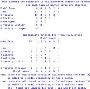
A.B.C. Model termmu (Mcode .) is a special case in that its test is conditional on all covariates but no factors. Following is someASRemloutput from the.aov

table which reports the terms in the conditional statistics.

Marginality pattern for F-con calculation Model terms

--Model Term DF 1 2 3 4 5 6 7 8

1 mu 1 * . . . .

2 water 1 I * C C . . c .

3 variety 7 I I * C . c . .

4 sow 2 I I I * C . . .

5 water.variety 7 I I I I * C C .

6 water.sow 2 I I I I I * C .

7 variety.sow 14 I I I I I I * .

8 water.variety.sow 14 I I I I I I I *

F-inc tests the additional variation explained when the term (*) is added to a model consisting of the I terms. F-con tests the additional variation explained when the term (*) is added to a model consisting of the I and C/cterms. Any

c terms are ignored in calculating DenDF forF-con using numericalderivatives for computational reasons. The . terms are ignored for both F-inc and F-con

tests.

Consider now a nested model which might be represented symbolically by

y∼1+REGION+REGION.SITE

For this model, the incremental and conditional Wald F statistics will be the same. However, it is not uncommon for this model to be presented toASRemlas

y∼1+REGION+SITE

ASREML user guide release 3.0

Rothamsted Repository Download

Gilmour, A. R., Gogel, B. J., Cullis, B. R. and Thompson, R. 2009.

ASREML user guide release 3.0. VSN International, Hemel Hempstead.

The publisher's version can be accessed at:

•

https://www.vsni.co.uk/downloads/asreml/release3/UserGuide.pdf

The output can be accessed at:

https://repository.rothamsted.ac.uk/item/8w146

.

© VSN International, Hemel Hempstead.

ASReml

User Guide

Release 3.0

2009

ASReml User Guide Release 3.0

Author email addresses

Copyright Notice

Published by:

Preface

Contents

List of Tables

List of Figures

1

Introduction

What ASReml can do

Installation

User Interface

How to use the guide

Help and discussion list

Typographic conventions

1.1

What ASReml can do

1.2

Installation

1.3

User Interface

1.4

How to use this guide

1.5

Getting assistance and the ASReml forum

1.6

Typographic conventions

2

Some theory

The linear mixed model

Estimation

What are

BLUP

s?

Combining variance models

Inference: Random effects

Inference: Fixed effects

2.1

The linear mixed model

2.2

Estimation

2.3

What are

BLUPs

?

2.4

Combining variance models

2.5

Inference: Random effects

2.6

Inference: Fixed effects

_Introduction

_{Some theory}