Vol. 11, No. 4, 2019 Article ID IJIM-1238, 9 pages Research Article
Adaptive Steffensen-like Methods with Memory for Solving Nonlinear
Equations with the Highest Possible Efficiency Indices
M. J. Lalehchini ∗, T. Lotfi †‡, K. Mahdiani §
Received Date: 2018-11-14 Revised Date: 2019-05-06 Accepted Date: 2019-07-06
————————————————————————————————–
Abstract
The primary goal of this work is to introduce two adaptive Steffensen-like methods with memory of the highest efficiency indices. In the existing methods, to improve the convergence order applied to memory concept, the focus has only been on the current and previous iteration. However, it is possible to improve the accelerators, considering the time from the first to the current iterations. Therefore, we achieve superior convergence orders and obtain as high efficiency indices as possible . These are the main contributions of this work.
Keywords: Nonlinear equations; Iterative methods; Steffensen-like method; Methods with memory; Adaptive methods; R-order.
—————————————————————————————————–
1
Introduction
O
ning numerical algorithms is to establish op-e of the most important subjects in develop-timal algorithms with economic complexity. For example, developing iterative methods for ap-proximating zero(s) of a given nonlinear equation falls within this matter, and many studies have been devoted to it [9, 12]. Inspired by this, we will set up two adaptive Steffensen-like methods with memory which are improvement of the ex-isting methods[1,5,6,12,16,22]. To our knowl-edge, these kinds of adaptive methods have not∗Department of Applied Mathematics, Hamedan
Branch, Islamic Azad University, Hamedan, Iran.
†Corresponding author. [email protected], Tel:
+98(918)8121361.
‡Department of Applied Mathematics, Hamedan
Branch, Islamic Azad University, Hamedan, Iran.
§Department of Applied Mathematics, Hamedan
Branch, Islamic Azad University, Hamedan, Iran.
been studied in the literature. Traub developed the first method with memory from Steffensen’s method [5] as following[11]:
wk=xk+γkf(xk),
xk+1=xk−f[xk,wk]f(xk) , k= 0,1,2,· · ·, γk+1=−N′ 1
1(xk+1),
(1.1) where x0 and γ0 are given initially suitable val-ues, and N1(t) =f(xk+1) + (t−xk+1)f[xk+1, xk] is the linear Newton’s interpolation. The con-vergence order of the with-memory method (1.1) is 1 +√2 ≈ 2.414. Also, Dˇzunni´c and Petkovi´c improved Traub’s idea, introducing a better ac-celerator [12]:
wk=xk+γkf(xk),
xk+1=xk−f[xk,wk]f(xk) , k= 0,1,2,· · ·, γk+1=−N′ 1
2(xk+1),
(1.2)
where x0 and γ0 are given initially suitable values, and N2(t) is the Net-won’s interpolation polynomial given by
N2(t) =f(xk+1) + (t−xk+1)f[xk+1, wk]+ (t−xk+1)(t−wk)f[xk+1, wk, xk].
The convergence order of the method with memory (1.2) is 1 +√4 = 3. Moreover, Dˇzuni´c added another parameter to the Steffensen’s method and obtained a more efficient method with memory [9]:
xk+1 =xk−f[xk,wk]+λkf(xk)f(wk), γk+1 =−N′ 1
2(xk+1), k= 0,1,2,· · ·,
wk+1 =xk+1+γk+1f(xk+1), λk+1 = −N
′′
3(wk+1)
2N3′(wk+1),
(1.3) where x0, γ0, and λ0 are given initially suitable values. This method has the convergence order
3+√17
2 ≈3.56.
Remark 1.1 If γ and λ are constants, then methods (1.2) and (1.3) are without memory methods with convergence order two having the following error equations, respectively:
ek+1 =c2(1 +γf′(α))e2k+O(e3k), (1.4) and
ek+1 = (c2+λ)(1 +γf′(α))e2k+O(e3k). (1.5)
In this work, we will attempt to carry out two adaptive methods with memory regardless of (1.2) and (1.3), which are superior [2,14,20,24]. To achieve this end,first, the accelerator param-eter γk is updated with the existing information in the previous and current iterations. We prove that this method has convergence order 3.4 us-ing the same function evaluations as (1.2), so its efficiency index is much better. Similarly, we de-rive another adaptive method with memory for (1.3) which acquires convergence order 3.9 using the same functional evaluations. Therefore, this method is better than both our adaptive method with one accelerator and all the existing methods.
2
Developing
adaptive
with
memory methods
This section deals with two new adaptive meth-ods with memory. To this end, we modify and
ex-tend methods (1.2) and (1.3) in such a way that they consider all previous information to attain as high as possible convergence order without any new functional evaluation. In this manner, we use the adaptive idea which has not been considered to our best knowledge.
2.1 Mono accelerator adaptive with memory method
In (1.2), to update accelerator γk in each itera-tion, we only use the information from the current and previous iterations and reach the convergence order 3. However, the procedure goes ahead, the old information of current and previous steps can be used. In another words, we tend to apply the adaptive idea to construct the new methods with memory. Accordingly, we introduce the following new adaptive method with memory
wk=xk+γkf(xk),
xk+1=xk−f[xk,wk]f(xk) , k= 0,1,2,· · ·, γk+1=−N′ 1
2k+2(xk+1),
(2.6) where x0 and γ0 are given initially suitable values, and N2k+2(t) is Netwon’s interpolation polynomial of degree 2k + 2 at the points xk+1, wk, xk, . . . , w0, x0. Referring to
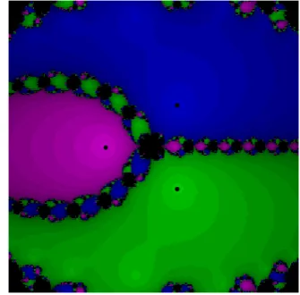
Figure 1: Dynamical Planes for (2.6) forγ= 0.1.
Table 1: Test functions for γ= 0.1,λ= 0.1.
Example x0 α
f1(t) =e(t
2−4)
+ sin(t−2)−t4+ 15 2.50 2.00
f2(t) = t14 −t2−
1
t+ 1 2.00 1.00
f3(t) = (t−2)(t10+t+ 2)e−5t 2.40 2.00
f4(t) =e(t
2−3t)
+ sin(t) + log (t2+ 1) 0.45 0.00
Table 2: Test functions for γ= 0.1,λ= 0.1.
Function. |x1−α| |x2−α| |x3−α| COC
f1 0.2371(0) 0.9503(-2) 0.1967(-7) 4.0683
f2 0.3417(-1) 0.9531(-3) 0.1021(-8) 3.8404
f3 0.2024(0) 0.2490(-2) 0.8749(-10) 3.9025
f4 0.2277(-1) 0.4709(-3) 0.3300(-9) 3.6537
Table 3: Results of (2.25) for different test functions.
Function. |x1−α| |x2−α| |x3−α| COC
f1 0.2902(0) 0.1028(-1) 0.1581(-7) 4.0078
f2 0.9073(-1) 0.2554(-2) 0.2200(-8) 3.9115
f3 0.1681(0) 0.1006(-2) 0.1582(-11) 3.9603
f4 0.4153(-1) 0.4718(-3) 0.5529(-11) 4.0784
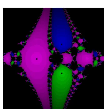
Figure 2: Dynamical Planes for (2.6) for γ = −0.31093.
Even if we assumed that α was known, we could not use it to evaluate f′(α), since it increased the functional evaluation, and optimality of the methods would be destroyed. It is assumed that the sequence{xk}converges toα. Moreover,f′ is at least continuous, so there is limf′(xk) =f′(α) as k→ ∞. Thus, we can useN2k+2′ (xk) instead off′(xk) to our mission, i.e.,γk =−1/N2k+2′ (xk).
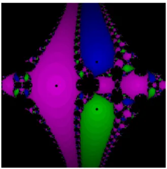
Figure 3: Dynamical Planes for (2.6) for γ = −0.33330.
To discuss the convergence order of (2.6), we need:
Figure 4: Dynamical Planes for (2.6) forγ= 0.1
Figure 5: Dynamical Planes for (2.6) for γ = −0.21435
λk+1= −
N2′′k+3(wk+1)
2N2′k+3(wk+1) then
1 +γf′(α)∼ k
∏
i=0
ew,iei, c2+λ∼ k
∏
i=0 ew,iei,
(2.7)
where ei=xi−α andew,i =wi−α.
Proof. According to Newton’s interpolation for-mula for nodes t0, t1, ..., ts,we have
f(t)−Ns(t) = f
(s+1)(ξ) (s+ 1)!
s
∏
i=0
(t−ti). (2.8)
where s ∈ [min{t0, t1, ..., ts},max{t0, t1, ..., ts}] and
γ =− 1
f′(α) ≃ − 1
N2k+2′ (xk) =γk+1. (2.9)
Figure 6: Dynamical Planes for (2.6) for γ = −0.24975
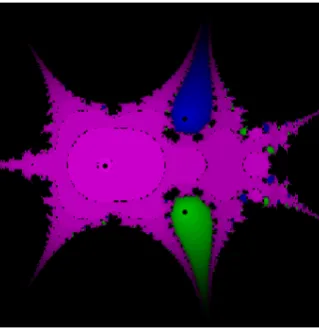
Figure 7: Dynamical Planes for (2.25) for γ = 0.1, λ= 0.1.
By differentiating (2.8) and setting t=xk+1 like proving Lemma 1 in [12], we have
N2k+2′ (xk+1) =f′(xk+1)−
f(2k+3)(ξ) (2k+ 3)! × k
∏
i=0
(xk+1−xi)(xk+1−wi)
∼f′(α)(1 +c2k+3 k
∏
i=0
ew,iei).
(2.10)
Consequently,
1 +γk+1f′(α) = 1− f
′(α)
N2k+2′ (xk+1) =
1− 1
1−c2k+3
∏k
i=0ew,iei ∼
k
∏
i=0 ew,iei.
Figure 8: Dynamical Planes for (2.25) for γ = −0.31336, λ= 0.99909.
Figure 9: Dynamical Planes for (2.25) for γ = −0.33334, λ= 1.
To prove the second relation with respect to (2.8),(2.10)and Lemma1 in [9] we have
c2+λk+1 = f′′(α) 2f′(α) −
N2k+3′′ (wk+1) 2N2k+3′ (wk+1)
∼ k
∏
i=0 ew,iei
(2.12)
Theorem 2.1 Let the initial approximation x0
be sufficiently close to the zeroαoff. AlsoRand
p denote the convergence order of the sequences
{xk} and{wk}, respectively, as obtained in
adap-tive method with memory (2.6). Then, we will have
{
Rkp−Rk−(p+ 1)∑ki=0−1Ri= 0, Rk+1−Rk−(p+ 1)∑k−1
i=0 Ri= 0.
(2.13)
Figure 10: Dynamical Planes for (2.25) forγ = 0.1, λ= 0.1
Figure 11: Dynamical Planes for (2.25) forγ = −0.21210, λ=−1.46997
Proof. We can assume
ek+1 ∼eRk. (2.14)
Hence,
ek+1 ∼(eRk−1)R=eRk−21. (2.15) Inductively,
ek+1∼eR0k+1. (2.16) Similarly, we have
ew,k∼epk= (eRk−1)p =e R p
k−1. (2.17) Thus,
ew,k∼eR kp
0 . (2.18)
By (2.14) and (2.17), Lemma 2.1 results in
1 +γf′(α)∼e(p+1)
∑k−1
i=0Ri
Figure 12: Dynamical Planes for (2.25) for γ = −0.25005, λ=−1.49993
On the other hand, since ew,k ∼ (1 +γf′(α))ek and ek+1 ∼ (1 +γf′(α))e2k, taking into account (2.19), we have
ew,k∼eR
k+(p+1)∑k−1
i=0Ri
0 , (2.20)
and
ek+1∼e2R
k+(p+1)∑k−1
i=0Ri
0 . (2.21)
From (2.18)-(2.20) and (2.16)-(2.21), we conclude that
eR0kp∼eR
k+(p+1)∑k−1
i=0R
i
0 , (2.22)
eR0k+1 ∼e2R
k+(p+1)∑k−1
i=0Ri
0 . (2.23)
Consequently,
{
Rkp−Rk−(p+ 1)∑ki=0−1Ri = 0,
Rk+1−2Rk−(p+ 1)∑ki=0−1Ri = 0. (2.24)
2.2 Bi accelerators adaptive with memory method
We now introduce bi accelerators adaptive with memory method [7,14,19,20,21,24]. Since most of the details are similar to the descriptions of (2.6), we confine ourselves to repeat them. We consider the following two new accelerators adap-tive with-memory method:
xk+1 =xk−f[xk,wk]+λkf(xk)f(wk), γk+1 =−N′ 1
2k+2(xk+1), k= 0,1,2,· · ·,
wk+1=xk+1+γk+1f(xk+1), λk+1 = −N2′′k+3(wk+1)
2N2′k+3(wk+1),
(2.25)
wherex0, γ0 andλ0 are given suitably. Then, we have
Theorem 2.2 Let the initial approximation x0
be sufficiently close to the zeroαoff. AlsoRand
p denote the convergence order of the sequences
{xk} and{wk}, respectively, as obtained in
adap-tive method with memory (2.25). Then, we will have
{
Rkp−Rk−(p+ 1)∑ki=0−1Ri= 0, Rk+1−2Rk−2(p+ 1)∑k−1
i=0 Ri = 0. (2.26)
Proof. We can assume
ek+1 ∼eRk. (2.27)
Hence,
ek+1 ∼(eRk−1)R=eR
2
k−1. (2.28) Inductively,
ek+1∼eR k+1
0 . (2.29)
Similarly, we have
ew,k∼epk= (eRk−1)p =eR pk−1. (2.30)
Thus,
ew,k∼eR0kp. (2.31) By (2.14) and (2.17), Lemma 2.1 results
(c2+λ)(1 +γf′(α))∼e2(p+1)
∑k−1
i=0Ri
0 . (2.32)
By (1.5)and ew,k ∼ (1 +γf′(α))ek , taking into account (2.32), we have
ew,k∼e
Rk+(p+1)∑k−1
i=0Ri
0 , (2.33)
and
ek+1∼e
2Rk+2(p+1)∑k−1
i=0Ri
0 . (2.34)
From (2.31)-(2.33) and (2.29)-(2.34), we conclude that
eR0kp∼eR
k+(p+1)∑k−1
i=0Ri
0 , (2.35)
eR0k+1 ∼e2Rk+2(p+1)
∑k−1
i=0Ri
0 . (2.36)
Consequently,
{
Rkp−Rk−(p+ 1)∑ki=0−1Ri = 0, Rk+1−2Rk−2(p+ 1)∑ki=0−1Ri = 0.
3
Numerical Computations
In this section, to show the efficiency of the new adaptive methods with memory (2.6) and (2.25), we report their numerical results. To this end, among many tested problems, we confine to re-port the results of four test functions (See Table
1). Moreover, the initial values are given in Ta-bles1. It should be noted that|xk−α|shows the error in each iteration anda(b) stands forab, and the computational order of convergence (COC) can been approximated by the following formula:
COC≈ log
|xk+1−α| |xk−α| log|xk|xk−α|
−1−α|
.
Tables2and3report the numerical implemen-tations of the adaptive methods with memory in this work. Table 2 shows that the numerical re-sults support the developed theory for method (2.6). As can be seen in Table 3, the (COC) of the tested functions using the method (2.25) is very good, and has the highest amount. Indeed, there is not any work in the literature that could compete with method (2.25). On the other hand, this is the highest and the best efficiency index which comes from the point of the efficiency in-dex. Let us discuss this contribution a little more. It is well known that any general optimal multi-point method without memory, usingn+ 1 func-tional evaluations has optimal convergence order 2n, so it could reach the optimal efficiency in-dex E∗(n+ 1,2n) = limn→∞2
n
n+1 = 2. On the other hand, we have proved that the new adaptive method with memory (2.25) could reach the same efficiency index with only two functional evalua-tions (See Theorem 2.2). This means that this method competes with any optimal multipoint method without memory.
In what follows, we disclose the mathematica code for the numerical implementations.
4
Dynamical Behavior
Here we focus on the stability behavior of the adaptive methods with memory (2.6) and (2.25). To this end, we utilize visual dynamical approach [13, 15, 17, 19, 24]. Although we have tested many examples, we have reached the same con-clusion. Therefore, we only report the results for
the function p(z) =z3+ 1 andp(z) =z4−1 . To show the stability of the one-parameter (2.6)and two-parameter (2.25) methods, we analyze their dynamic properties and focus on the of dynamic planes related to iterative methods. Mathematica software can be used to do the analysis in which the graphic planes are shown in a rectangle of [−3,3]×[−3,3] dimension along with a 72-pixel resolution. The dynamic planes illustrate the ab-sorption area for polynomialsp1(z) =z3+ 1 and p2(z) =z4−1. p1(z) andp2(z) have the solution of −1,12(1 +i√3),12(1−i√3) and−1,1,−i, i, re-spectively. Each solution is allocated a color. The greater the dark areas, the greater the intensity of unstability. In Figures 1, 2 and 3, the stabil-ity of single parameter methods (2.6) is shown for γ = 0.1,−031093 and−0.3333, in whichp1(z) has been used. Also, in Figures4,5and6, the stabil-ity of single parameter method (2.6) is shown for γ = 0.1,−0.31336 and−0.33334 in whichp2(z) is used. Comparing the figures shows that the sta-bility has been reduced. For the two-parameter method (2.25), in Figure 7, the absorption area and stability are shown forγ andλat 0.1 and 0.1 respectively, in Figure 8 for γ = −0.31336 and λ = 0.99909 and in Figure 9 for γ = −0.33334 and λ = 1.00000, where p1(z) is used. Finally, the two-parameter iterative method (2.25) has been taken to compare absorption areas, using p2(z) in Figures 10,11 and 12, forγ and λat 0.1 and 0.1 in Figure 10, -0.21210 and -1.46997 in Figure (11) and -0.25005, -1.49993 in Figure 12, where p2(z) is used. comparing the figures, we witness there is a reduction in stability showing that, despite the increase of convergence order in the two-parameter method (2.25), the stabil-ity trend is satisfactory. Both developed meth-ods with memory (2.6) and (2.25) show the same instable behavior. Consequently, though devel-oping methods with memory has the advantage from the view of computational complexity, they represent numerical chaos and numerical instabil-ity.
5
Conclusion
could reach the highest possible efficiency indices and can compete with any method with or with-out memory in the literature. Convergence analy-sis of the developed methods has been presented, and we have tested some numerical examples to show the practicality of the proposed methods. Though both developed methods have the highest possible efficiency as opposed to any other meth-ods in the literature, we have seen that methmeth-ods with memory show instability in practice. There-fore, they benefit from computational efficiency and suffer from numerical stability. Finally, we end the conclusion with the following research question: how can a method with memory be de-veloped to show the numerical stability behavior?
References
[1] A. Cordero, J. R. Torregrosa, A class of Stef-fensen type methods with optimal order of convergence,Applied Mathematics and Com-putation 19 (2011) 7653-7659.
[2] A. Cordero, T. Lotfi, P. Bakhtiari, J. R. Tor-regrosa, An efficient two-parametric family with memory for nonlinear equations, Nu-mer. Algorithms 68 (2015) 323-335.
[3] H. T. Kung, J. F. Traub , Optimal order of one-point and multipoint iteration, J. ACM
21 (1974) 643-651 .
[4] H. Veiseh, T. Lotfi, T. Allahviranloo, A study on the local convergence and dy-namics of the two-step and derivative-free Kung Traubs method (2017). http://dx. doi.org/10.1007/s40314-017-0458-5/.
[5] I. F. Steffensen, Remarks on iteration,
Skand. Aktuarietidskr 16 (1933) 64-72.
[6] I. K. Argyros, H. Ren, Efficient Steffensen-type algorithms for solving nonlinear equa-tions, International Journal of Computer Mathematics 90 (2013) 691-704.
[7] I. K. Argyros, M. Kansal, V. Kanwar, S. Bajaj, Higher-order derivative-free families of Chebyshev Halley type methods with or without memory for solving nonlinear equa-tions, Applied Mathematics and Computa-tion 315 (2017) 224-245.
[8] I. K. Argyros, S. George, A. A. Ma-grenan, Local convergence for multi-point-parametric Chebyshev-Halley-type methods of high convergence order, Journal of
Com-putational and Applied Mathematics 282
(2015) 215-224.
[9] J. Dzunic, On efficient two-parameter meth-ods for solving nonlinear equations, Numer-ical Algorithms 63 (2013) 549-569.
[10] J. Dzunic, M. S. Petkovic, A cubically con-vergent steffensen-like method for solving nonlinear equations, Applied Mathematics Letters 25 (2012) 1881-1886.
[11] J. F. Traub, Iterative methods for the solu-tion of equasolu-tions, Prentice-Hall, Englewood Cliffs, New Jersey, 1964.
[12] M. S. Petkovic, B. Neta , L. D. Petkovic , J. Dzunic, Multipoint methods for solving nonlinear equations: a survey, Appl. Math. Comput.226 (2014) 635-660.
[13] M. Salimi, T. Lotfi, S. Sharifi, S. Siegmund, Optimal Newton Secant like methods with-out memory for solving nonlinear equations with its dynamics, International Journal of Computer Mathematics94 (2017) 1759-1777.
[14] M. Zaka Ullah, S. Kosari, F. Soleymani, F. Khaksar Haghani, A. S. Al-Fhaid, A super-fast tri-parametric iterative method with memory, Applied Mathematics and Compu-tation 289 (2016) 486-491.
[15] P. Bakhtiari, A. Cordero, T. Lotfi, K. Mahdi-ani, J. R. Torregrosa, Widening basins of at-traction of optimal iterative methods, Non-linear Dynamics 87 (2017) 913-938.
[16] S. Artidiello, A. Cordero, J. Torregrosa, M. Vassileva, Two weighted eight-order classes of iterative root-finding methods, Interna-tional Journal of Computer Mathematics 92 (2015) 1790-1805.
[18] S. Amat, S. Busquier, J. M. Gutierrez, On the local convergence of secant-type methods, International Journal of Computer Mathematics 81 (2004) 1153-1161.
[19] S. Aridiello, F. Chicharro, A. Cordero, J. Torregrosa,Local convergence and dy-namical analysis of a new family of opti-mal fourth-order iterative methods, Interna-tional Journal of Computer Mathematics 90 (2013) 2049-2060.
[20] T. Lotfi, F. Suleiman, M. Ghorbanzadeh, P. Assari, On the construction of some tri-parametric iterative methods with memory,
Numer. Algorithms 70 (2015) 835-845.
[21] T. Lotfi, F. Soleymani, Z. Noori, A. Kman, F. Khaksar Haghani, Efficient iterative methods with and without memory possess-ing high efficiency indices,Discrete Dynam-ics in Nature and Society 9 (2014) 20-34.
[22] T. Lotfi, K. Mahdiani, P. Bakhtiari, F. Soleymani, Constructing two-step iterative methods with and without memory, Com-putational Mathematics and Mathematical Physics 55 (2015) 183-193.
[23] T. Lotfi, P. Bakhtiari, A. Cordero, K. Mah-diani, J. R. Torregrosa, Some new efficient multipoint iterative methods for solving non-linear systems of equations, International Journal of Computer Mathematics 92 (2015) 1921-1934.
[24] X. Wang, T. Zhang, Y. Qin, Efficient two-step derivative-free iterative methods with memory and their dynamics, International Journal of Computer Mathematics 93 (2016) 1423-1446.
[25] Y. H. Geum , Y. I. Kim , B. Neta , On developing a higher-order family of double-Newton methods with a bivariate weighting function, Appl. Math. Comput. 254 (2015) 277-290.
Mohammad Javad Lalehchini is a PhD candidate in Department of Applied Mathematics, Hamedan Branch, Islamic Azad University, Hamedan, Iran. Her research ar-eas in Numerical analysis is include approximating numerical solutions using iterative methods for nonlinear systems of equations.
Taher Lotfi has got MSc de-grees in Applied Mathematics from Kharazmi (Tarbiat Moallem) Uni-versity, and PhD degree from Sci-ence and Research Branch, Islamic Azad University, Tehran, Iran. My main research interest include ap-proximating numerical solutions using iterative methods for nonlinear systems of equations, spe-cially for large systems arising from IE, ODE and PDE. Also, interval analysis, reproducing kernel space methods, soft computing based on wavelets and fuzzy concepts, generalized inverses are my current MSc and PhD students research field.