DEMOGRAPHIC RESEARCH
A peer-reviewed, open-access journal of population sciences
DEMOGRAPHIC RESEARCH
VOLUME 39, ARTICLE 23, PAGES 671–684
PUBLISHED 27 SEPTEMBER 2018
http://www.demographic-research.org/Volumes/Vol39/23/ DOI: 10.4054/DemRes.2018.39.23
Formal Relationship 27
The impact of proportional changes in
age-specific mortality on life expectancy when
mortality is a log-linear function of age
Michael Væth
Mette Vinther Skriver
Henrik Støvring
c
2018 Væth, Skriver & Støvring.
This open-access work is published under the terms of the Creative Commons Attribution 3.0 Germany (CC BY 3.0 DE), which permits use, reproduction, and distribution in any medium, provided the original author(s) and source are given credit.
1 Relationship 672
2 Proof 672
2.1 Comments 673
3 Robustness of the result 674
4 Previous work on the relation between mortality rate and life expectancy 676
5 An application 677
The impact of proportional changes in age-specific mortality on life
expectancy when mortality is a log-linear function of age
Michael Væth1
Mette Vinther Skriver2
Henrik Støvring2
Abstract
BACKGROUND
Demographers and epidemiologists have investigated the dependence of life expectancy on proportional changes in the age-specific mortality.
OBJECTIVE
To develop an approach that allows estimation of change in life expectancy from pro-portional changes in age-specific mortality and to identify aspects of the death rate that influence the accuracy of the estimation.
RESULTS
We obtain an exact expression for the first derivative of the life expectancy with respect to the proportional change in age-specific mortality when the age-specific death rate is log-linear in age. We use the result to establish bounds for the change in life expectancy following a proportional change of the mortality. The result shows that the change in life expectancy is approximately linear in the logarithm of the proportional change of the mortality. In populations with low infant mortality, the slope of this linear relationship is essentially equal to minus the inverse of the slope of the log-linear age dependence of the death rate.
CONTRIBUTION
In a wide range of mortality scenarios, the relationship between change in life expectancy and the logarithm of the proportional change of the mortality allows accurate approxima-tion of a difference in life expectancy from a ratio of death rates.
1. Relationship
Assume that lifetime from a given age,a, follows a Gompertz distribution whose age-specific death rate is defined asm(x) =αeβ(x−a)at agex≥aand letκ=α β−1.
Consider a proportional change of age-specific mortality by a constant cand let
e(a;c)denote life expectancy at ageawhen the age-specific death rate ismc(x) =cm(x).
The change in life expectancy introduced by the proportional changecin age-specific mortality then satisfies the following inequalities:
(1) β−1log(c)h(cκ)<e(a; 1)−e(a;c)<β−1log(c)h(κ), withh(x) =1−xexE1(x), whereE1(x) =
R∞
x e
−z
z dzis the exponential integral.
2. Proof
Consider life expectancy as a function ofb=log(c). The mean value theorem then gives
(2) e(a;c)−e(a; 1) = (b−0)Dbe(a; exp(b∗)),
where the first derivative with respect tobis computed for someb∗ε[0,b]. To establish the inequalities, we show that life expectancye(a;c)is a decreasing, convex function of
bsuch that the first derivative atb∗is bounded between the values of the first derivative at the boundary of the interval.
It is well-known (see, e.g., Broadbent 1958) thate(a; 1) =β−1eκE1(κ). If the age-specific mortality is changed by a factor ofcfor agesx≥a, lifetime follows a Gompertz distribution with parameterscα,β. Therefore,
(3) e(a;c) =β−1exp(cκ)E1(cκ).
Straightforward calculations give
(4) Dbe(a;c) =−β−1[1−cκecκE1(cκ)] =−β−1h(cκ), and
D2be(a;c) =β−1[cκecκE
From Temme (2010) we have (see formula 6.8.2)
x x+1 <xe
xE
1(x)<
x+1
x+2,
so(x+2)−1<h(x)<(x+1)−1showing thatDbe(a;c)<0. Moreover, the second
deriva-tive satisfies the inequalities
0<D2be(a;c)<β−1(cκ+2)−1,
and the first derivative is therefore an increasing function ofb, i.e.,
Dbe(a; 1)<Dbe(a; exp(b∗))<Dbe(a;c).
The result in (1) then follows by applying these inequalities to (2) and rearranging terms.
2.1 Comments
For small values ofcκandκ, the inequalities in (1) are very tight. The derivation above shows that the correction factorh(x)is a decreasing function ofx. Moreover, lim
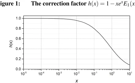
x→0h(x) =1 and, using the power series representation ofE1(x)– see Temme (2010), formula 6.6.2 – it follows thath(x)behaves like 1+xlog(x)asx→0. In particular, ifcκandκare both less than 0.0017, then the ratio of the lower bound to the upper bound in (1) is between 0.99 and 1. Consequently, the change in life expectancy is essentially proportional to log(c)with−β−1as the constant of proportionality. Figure 1 shows the behavior ofh(x)
in the range from 0+ to 10.
Figure 1: The correction factorh(x) =1−xexE1(x)forx<10
3. Robustness of the result
The distribution of lifetimes in human populations differs from that predicted by a Gom-pertz distribution because of a higher mortality in childhood and for young adults. More-over, the slope of the log-linear age relation of the mortality rate is reduced for very old ages. The sensitivity of the main result to such deviations is therefore of some interest. To this end we consider the impact of two mathematically tractable modifications of the death rate.
A simple modification that allows higher mortality at young ages may be obtained by assuming a constant death ratem(x) =αfor agesx≤A. For agesx>A, the log-linear age dependence takes over such thatm(x) =αeβ(x−A). Note that this modification sets the death rate for ages younger thanAto the death rate at ageAfor the Gompertz model. Life expectancy at birth in this distribution becomes
(5) eA(0) =α−1(1−e−αA) +e−αAβ−1eκE1(κ) =α−1(1−e−αA) +e−αAe(A; 1), whereκ =α β−1 ande(A; 1) are defined in (3). Note that in this model,e−αA is the
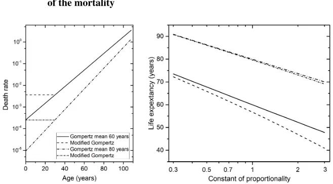
probability of surviving until ageA. Replacingαbycαintroduces a proportional change of the mortality, and the change in life expectancy as a function ofb=log(c)may then be studied. Figure 2 shows the results for two scenarios in which a Gompertz distribution has been modified to have a constant death rate for ages below 30. The solid curve in the right panel shows the relation for a Gompertz distribution with life expectancy 60 years and a probability of surviving until age 30 years ofp(30) =0.963. A similar modification is shown for a Gompertz distribution with life expectancy 80 years and p(30) =0.998. The modification of the Gompertz distribution with mean 80 years has almost no impact on the relationship, but for the other scenario the effect is clearly visible, in particular for
Figure 2: Death rates and life expectancy as a function of a proportional change of the mortality
Note: The left panel shows the death rate of a Gompertz distribution with mean 60 years, (α,β) = (2.562× 10⁻⁴, 0.088), a modification of this distribution withm(x) =3.591×10⁻³forx<30, a Gompertz distribution with mean
80 years,(α,β) = (9.317×10⁻⁶, 0.11), and a modification of this distribution withm(x) =2.526×10⁻⁴forx<30. For
these four distributions, the right panel shows the relation betweenlog(c)and the change in life expectancy at birth for0.3<c<3(equations (3) and (5)).
The impact of a reduced log-linear slope at old ages may conveniently be studied by assuming thatm(x) =αeβ(x−a) fora≤x<Bandm(x) =α
Beβ1(x−B)forx>B, where
αB=αeβ(B−a). In this distribution, the life expectancy at ageais given by
(6) eB(a) =β−1eκE1(κ) +p(B|a)(β1−1eκ2E
1(κ2)−β−1eκ1E
1(κ1)),
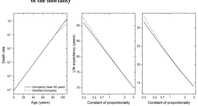
Figure 3: Death rates and life expectancy as a function of a proportional change of the mortality
Note: The left panel shows the death rate of a Gompertz distribution with mean 80,(α,β) = (9.317×10⁻⁶, 0.11), and
of a modification for which the log-linear slope is reduced by 30% for ages above 85. For0.3<c<3, the center panel shows the life expectancy at birth as a function oflog(c), and the right panel shows the life expectancy at age 60 years as a function oflog(c), cf. equations (3) and (6).
Figure 3 illustrates the relation between log(c)and the life expectancy at birth (center panel), and at age 60 years (right panel), when there is a 30% decrease in the log-linear slope at ages above 85 years. The unmodified Gompertz distribution is identical to the distribution with mean 80 years used in Figure 2. In this distribution the probability of surviving until age 85 years is 0.378. The probability becomes smaller when c increases, and the modification therefore has little or no impact forc>1. Forc<1, the slope in Figure 3 becomes steeper and, ascdecreases, approaches the value of minus the inverse of the modified log-linear slope. This modification introduces some curvature.
While not exhaustive, the results of this sensitivity study suggest that the approxi-mately linear relation between log(c)and life expectancy is relatively robust to the type of deviations from a Gompertz distribution observed in human populations.
4. Previous work on the relation between mortality rate and life
expectancy
changes in life expectancy due to small proportional changes in the total or cause-specific mortality have been described by Keyfitz (1977, 1985), Vaupel (1986), and Vaupel and Canudas Romo (2003). These and other results have been summarized by Wrycza and Baudisch (2012), who also present results on changes in life expectancy that are intro-duced by other types of perturbations in age-specific mortality.
Demographers are often interested in the dynamics of populations, and their focus is therefore on describing the impact of small changes on population parameters from one calendar year to the next. Epidemiologists have also studied the impact of changes in the age-specific mortality on life expectancy, but their purpose has been different. In epidemiology, both the life expectancy and the standardized mortality ratio (SMR) are used as mortality indices for population comparisons, and a relationship between them would allow a translation of results from one index to the other. Tsai, Hardy, and Wen (1992) and Lai, Hardy, and Tsai (1996) used regression methods to establish an empirical relation between SMR and life expectancy, whereas Haybittle (1998) applied a result for Gompertz distributions developed by Pollard (1991) to obtain an approximate linear dependency of life expectancy on the logarithm of the SMR. Our main result allows a study of the validity of their approximations.
Spiegelhalter (2016) presented a result closely related to our results. Assuming a log-linear age dependency of the death rate, he showed that the effect of a proportional change of the death rate by a constantccan be expressed as an adjustment of the current age by β−1log(c)years, whereβis the slope of the log-linear age dependence. He described this adjusted age as the “effective age,” and advocated its use for risk communication. Thus, Spiegelhalter described the effect of the mortality change by moving the starting point of the remaining lifetime, whereas our approach involves changing the expected endpoint of the remaining lifetime.
5. An application
In a human population, let p(x)denote the probability of surviving until agex. After a proportional change of the mortality by a factor ofc, life expectancy at age a becomes
(7) a(a;c) =
Z ∞
a
p(x|a)cdx, wherep(x|a) =p(x)/p(a).
The results in the previous sections suggest thate(a;c)is approximately linear in log(c). When we therefore introduce a proportional change to the mortality by a factor of
c, the change in life expectancy at ageawill to a close approximation be equal to
whereKis the slope of the change.Kis equal to the first derivative of the life expectancy with respect tob=log(c)computed atb=0, i.e.,
(9) K=
Z ∞
a
log(p(x|a))p(c|a)dx.
To study the validity of the linear approximation (8) in a range of mortality scenar-ios, we consider data on Swedish women in three periods, 1910–1914, 1960–1964, and 2010–2014. From the Human Mortality Database (Human Mortality Database 2017), we obtained period life tables based on one-year age categories including data on number of deaths, exposure to risk, and mortality rates. The final age category was 110+ years. Fig-ure 4 shows the death rates for the three periods as a function of age. (Note the log-scale on the y-axis.) For adult ages, the logarithm of the death rate is approximately linear in age.
Figure 4: Death rates for Swedish women in the periods 1910–1914, 1960–1964,
and 2010–2014
Source: Human Mortality Database 2017.
computed from the life table using formula (7) with agea = 10, 30, 50, and 70. The curves are remarkably linear, in particular for the periods 1960–1964 and 2010–2014. For these periods, the slope of the change in life expectancy at age 70 is less steep, and the curve is slightly convex. For the earliest period, the slopes differ more, and some curvature is notable for age 10 and age 70.
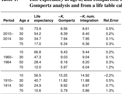
Two approaches were used to estimate the constantK, a direct life table calculation based on numerical integration of the right side of (9), and an approach relying on the relationK=−h(κ)β−1 for a Gompertz distribution, cf. formula (4). The Gompertz model was fitted by a Poisson regression model with logarithmic link function, number of deaths as the dependent variable, and the logarithm of the exposure to risk as an offset. For each period, the analysis was carried out for agesa= 10, 30, 50, and 70. Stata version 14 was used for all analyses (StataCorp 2015).
Figure 5: Change in life expectancy at agea;a= 10, 30, 50, and 70 as a function of a proportional change of the mortality rate
Note: Change in life expectancy computed from equation (7). Note the log-scale on the x-axis. Source: Swedish females 1910–1914, 1960–1964, and 2010–2014; Human Mortality Database 2017.
Table 1: Life expectancy at agea, and comparison of –Kestimated from a Gompertz analysis and from a life table calculation
Life –K, –K, num.
Period Agea expectancy Gompertz integration Rel.Error
10 73.9 8.56 8.61 0.5%
2010– 30 54.2 8.39 8.40 0.2%
2014 50 34.7 7.94 7.95 0.1%
70 17.0 6.34 6.36 0.3%
10 66.8 9.43 9.44 0.2%
1960– 30 47.3 9.03 9.04 0.1%
1964 50 28.4 8.18 8.20 0.3%
70 12.0 5.97 6.04 1.2%
10 56.5 15.25 14.92 –2.2%
1910– 30 40.7 11.82 11.88 0.5%
1914 50 24.9 8.92 8.97 0.7%
70 10.6 5.79 5.86 1.3%
Note: In the Gompertz analysis. –Kis estimated as−h(κ)β−1.
Source: Swedish women 1910–1914, 1960–1964, and 2010–2014; Human Mortality Database 2017.
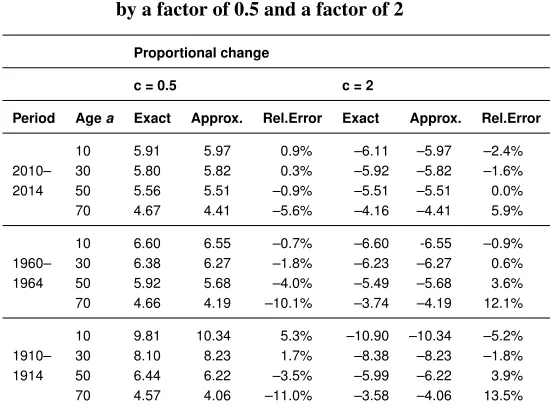
According to the Swedish life table for the period 2010–2014, life expectancy is 54.17 years for a woman at age 30. If the age-specific death rates are reduced by 50%, the life expectancy obtained by numerical integration of (7) becomes 59.98 years, and the linear approximation (8) leads to 60.00 years. For the three periods considered here, Table 2 compares the exact change in life expectancy at agea= 10, 30, 50, and 70, obtained with numerical integration and the approximate value derived from the linear approximation (8) when the age-specific death rate is reduced by 50% or increased by a factor of 2. The results in Table 2 show that the linear approximation (8) provides an accurate estimate of the change in life expectancy following a relatively large proportional change of the mortality, in particular when the life expectancy is computed from age 30 or age 50. As expected, the accuracy seems to be highest when infant mortality is small.
Table 2: Comparison of exact values and approximate values of the change in life expectancy at ageafollowing a proportional change in death rates by a factor of 0.5 and a factor of 2
Proportional change
c = 0.5 c = 2
Period Agea Exact Approx. Rel.Error Exact Approx. Rel.Error
10 5.91 5.97 0.9% –6.11 –5.97 –2.4%
2010– 30 5.80 5.82 0.3% –5.92 –5.82 –1.6%
2014 50 5.56 5.51 –0.9% –5.51 –5.51 0.0%
70 4.67 4.41 –5.6% –4.16 –4.41 5.9%
10 6.60 6.55 –0.7% –6.60 -6.55 –0.9%
1960– 30 6.38 6.27 –1.8% –6.23 –6.27 0.6%
1964 50 5.92 5.68 –4.0% –5.49 –5.68 3.6%
70 4.66 4.19 –10.1% –3.74 –4.19 12.1%
10 9.81 10.34 5.3% –10.90 –10.34 –5.2%
1910– 30 8.10 8.23 1.7% –8.38 –8.23 –1.8%
1914 50 6.44 6.22 –3.5% –5.99 –6.22 3.9%
70 4.57 4.06 –11.0% –3.58 –4.06 13.5%
Note: Approximate values are based on equation (8).
Source: Mortality data on Swedish women 1910–1914, 1960–1964, and 2010–2014; Human Mortality Database 2017.
References
Broadbent, S. (1958). Simple mortality rates.Applied Statistics7(2): 85–96.doi:10.2307/ 2985310.
Haybittle, J. (1998). The use of the Gompertz function to relate changes in life expectancy to the standard mortality ratio.International Journal of Epidemiology27(5): 885–889.
doi:10.1093/ije/27.5.885.
Human Mortality Database (2017). Human mortality database. [electronic resource]. Berkeley and Rostock: University of California and Max Planck Institute for Demo-graphic Research.http://www.mortality.org.
Karn, M. (1931). An inquiry into various death rates and the comparative influence of cer-tain diseases on the duration of life.Annals of Eugenics4(3–4): 279–302.doi:10.1111/ j.1469-1809.1931.tb02080.x.
Keyfitz, N. (1977). What difference would it make if cancer were eradicated? An exami-nation of the Taeuber paradox.Demography14(4): 411–418.
Keyfitz, N. (1985).Applied mathematical demography. New York: Springer.
Lai, D., Hardy, R., and Tsai, S. (1996). Statistical analysis of the standardized mortal-ity ratio and life expectancy. American Journal of Epidemiology 143(8): 832–840.
doi:10.1093/oxfordjournals.aje.a008822.
Pollard, J. (1991). Fun with Gompertz.Genus47(1–2): 1–20.
Skriver, M., Væth, M., and Støvring, H. (2018). A method to estimate differences in life expectancy from a standardized mortality ratio.Scandinavian Journal of Public Health
(forthcoming).doi:10.1177/1403494817749050.
Spiegelhalter, D. (2016). How old are you, really? Communicating chronic risk through ‘effective age’ of body and organs. BMC Medical Informatics and Decision Making
16: 104.doi:10.1186/s12911-016-0342-z.
StataCorp (2015). Stata: Release 14: Statistical software. College Station: StataCorp.
Temme, N. (2010). Exponential, logarithmic, sine, cosine integrals. In: Olver, F., Lozier, D., Boisvert, R., and Clark, C. (eds.).NIST handbook of mathematical functions. New York: Cambridge University Press: 150–156.
Tsai, S., Hardy, R., and Wen, C. (1992). The standardized mortality ratio and life expectancy. American Journal of Epidemiology 135(7): 824–830. doi:10.1093/ oxfordjournals.aje.a116369.
Popu-lation Studies40: 147–157.doi:10.1080/0032472031000141896.
Vaupel, J. and Canudas Romo, V. (2003). Decomposing change in life expectancy: A bouquet of formulas in honor of Nathan Keyfitz’s 90th birthday. Demography40(3): 201–216.doi:10.2307/3180798.