Stratification of the severity of critically ill patients with classification trees

(1)

Open Access

Research article

Stratification of the severity of critically ill patients with

classification trees

Javier Trujillano*

1,2

_{, Mariona Badia}

1

_{, Luis Serviá}

1

_{, Jaume March}

3

_and

Angel Rodriguez-Pozo

1

Address: 1_{Intensive Care Unit, Hospital Universitario Arnau de Vilanova, IRBLLEIDA, (Avda Rovira Roure 80), Lleida (25198), Spain,}

2_{Departamento de Ciencias Médicas Básicas, Universidad de Lleida, (Avda Rovira Roure 44), Lleida (25006), Spain and}3_{Departamento de Cirugía,} Universidad de Lleida, (Avda Rovira Roure 80), Lleida (25198), Spain

Email: Javier Trujillano* - [email protected]; Mariona Badia - [email protected]; Luis Serviá - [email protected]; Jaume March - [email protected]; Angel Rodriguez-Pozo - [email protected]

* Corresponding author

Abstract

Background: Development of three classification trees (CT) based on the CART (Classification

and Regression Trees), CHAID (Chi-Square Automatic Interaction Detection) and C4.5 methodologies

for the calculation of probability of hospital mortality; the comparison of the results with the APACHE II, SAPS II and MPM II-24 scores, and with a model based on multiple logistic regression (LR).

Methods: Retrospective study of 2864 patients. Random partition (70:30) into a Development Set (DS) n = 1808 and Validation Set (VS) n = 808. Their properties of discrimination are compared with the ROC curve (AUC CI 95%), Percent of correct classification (PCC CI 95%); and the calibration with the Calibration Curve and the Standardized Mortality Ratio (SMR CI 95%).

Results: CTs are produced with a different selection of variables and decision rules: CART (5 variables and 8 decision rules), CHAID (7 variables and 15 rules) and C4.5 (6 variables and 10 rules). The common variables were: inotropic therapy, Glasgow, age, (A-a)O2 gradient and antecedent of chronic illness. In VS: all the models achieved acceptable discrimination with AUC above 0.7. CT: CART (0.75(0.71-0.81)), CHAID (0.76(0.72-0.79)) and C4.5 (0.76(0.73-0.80)). PCC: CART (72(69-75)), CHAID (72(69-75)) and C4.5 (76(73-79)). Calibration (SMR) better in the CT: CART (1.04(0.95-1.31)), CHAID (1.06(0.97-1.15) and C4.5 (1.08(0.98-1.16)).

Conclusion: With different methodologies of CTs, trees are generated with different selection of variables and decision rules. The CTs are easy to interpret, and they stratify the risk of hospital mortality. The CTs should be taken into account for the classification of the prognosis of critically ill patients.

Published: 9 December 2009

BMC Medical Research Methodology 2009, 9:83 doi:10.1186/1471-2288-9-83

Received: 22 February 2009 Accepted: 9 December 2009

This article is available from: http://www.biomedcentral.com/1471-2288/9/83

(2)

Background

Stratifying the patients into risk groups, according to their severity, is essential for the comparison of treatments and the establishment of differences between different units or hospital centres. As a result, working in an intensive care unit (ICU) necessitates making prognoses for patients within the first 24 hours of their admission. Establishing a prognosis consists of assigning a probability of death by using variables commonly used for the diagnosis and treatment of critically ill patients [1].

Severity scores are classic tools used in establishing this probability. The most commonly used scores are the APACHE II (Acute Physiology and Chronic Health Evaluation II), the SAPS II (Simplified Acute Physiology Score II) and the MPM II-24 (Mortality Probability Models II-24) scores [2-4].

Other systems of severity classification based on different mathematical strategies have also been used [5].

In the last decade, classification trees (CT), which were developed more than 20 years ago, have acquired greater importance in the immediate interpretation of the deci-sion rules that they generate, and they are readily accepted by professionals in clinical practice [6].

A CT is a graphic representation of a series of decision rules. Beginning with a root node that includes all cases, the tree branches are divided into different child nodes that contain a subgroup of cases. The criterion for branch-ing (or partitionbranch-ing) is selected after examinbranch-ing all possi-ble values of all availapossi-ble predictive variapossi-bles. In the terminal nodes (the "leaves" of the tree), a grouping of cases is obtained, such that the cases are as homogeneous

as possible with respect to the value of the dependent var-iable [7].

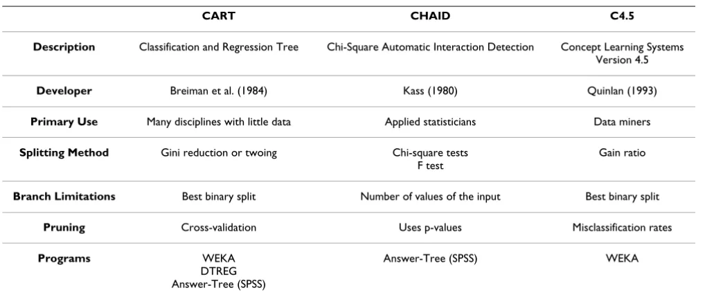
The different CT types are distinguished by the manner of node partitioning. In the specific case of CARTs ( Classifi-cation And Regression Trees), possibly the most widely used CT in medicine, an impurity function (the so-called Gini index) is calculated, and for each division of the tree, the variable and its cut-off value are defined such that the decrease in the impurity function is the greatest [8]. There are many types of CTs (or improved versions) such as CHAID (Chi-square Automatic Interaction Detection) and C4.5 (developed from the so-called Concept Learning Sys-tems). Table 1 illustrates, in a schematic fashion, the par-ticularities of these CTs. A CT has a growth phase, a pruning phase (removal of branches that do not provide general information to the system) and a selection of the optimal tree [8].

The aim of the present study was to develop (with a pop-ulation of critically ill patients) three classification trees (based on CART, CHAID and C4.5 methodologies) to cal-culate the probability of hospital mortality and to com-pare these trees with each other, with the classic scores (APACHE II, SAPS II and MPM II-24) and with a model based on multiple logistic regression.

Methods

This is a retrospective study carried out using the database of a mixed ICU (with medical and surgical services) of 14 beds located at the University Hospital Arnau de Vilanova of Lleida. The ethical committee of the hospital was informed that the study was being carried out, and informed consent was not deemed necessary, since all the

Table 1: Characteristics of the classification tree methods

CART CHAID C4.5

Description Classification and Regression Tree Chi-Square Automatic Interaction Detection Concept Learning Systems Version 4.5

Developer Breiman et al. (1984) Kass (1980) Quinlan (1993)

Primary Use Many disciplines with little data Applied statisticians Data miners

Splitting Method Gini reduction or twoing Chi-square tests F test

Gain ratio

Branch Limitations Best binary split Number of values of the input Best binary split

Pruning Cross-validation Uses p-values Misclassification rates

Programs WEKA

DTREG Answer-Tree (SPSS)

(3)

variables were collected for the diagnosis and treatment of the patients and their anonymity was assured at all times.

Database

Data collected over ten years (from January 1997 to December 2006) were used. In this study, all patients were over the age of 16 years and remained in the ICU for more than 24 hours. Patient records with incomplete data were not used.

A random partition, in a 70:30 ratio, was made to estab-lish the development and the validation sets, respectively.

Data concerning age, sex, length of stay in the ICU and procedures specific to the ICU were used. The outcome variable of interest was the probability of hospital mortal-ity. The patients were divided according to their diagnostic groups following the Knaus classification [9]. Six diagnos-tic groups were established according to the case mix and level of severity of the ICU, including two trauma catego-ries of TBI (traumatic brain injury) and Multiple trauma (multiple trauma without brain injury), Respiratory

(chronic respiratory problems with decompensation),

Neurological (ischemic or hemorrhagic strokes), Surgery

(surgical problems not included in other categories) and

Medicine (medical pathology not included in other cate-gories).

Each patient's medical records and laboratory database files were used to obtain information pertaining to base-line (at ICU admission) demographics, pre-existing comorbidities and scores (APACHE II, SAPS II and MPM II-24). The data were then compiled (manual recording) into single data using a relational database management system (Microsoft Access©).

APACHE II, SAPS II and MPM II-24 scores were deter-mined by the worst value found during the first 24 hours after ICU admission [2-4].

The presence of acute renal failure was defined (according to the model MPM II-24) by levels of serum creatinin above 2 mg/dL [4]. The antecedents of chronic organ insufficiency (defined according to the APACHE II model) were included in the variable COI [2].

Logistic models and classification trees

Models were created with the development set and were subsequently checked in the validation set.

Working with the development set, first, a univariate anal-ysis was performed for all the variables included in the three scores to select those that predicted survival. Those that were statistically significant predictors were included in the development of the multivariable models.

We used a model of multiple logistic regression (LR) with forward stepwise selection of variables [10].

The computer programs used for creating the CTs are pre-sented in Table 1. The program WEKA (a project of Waikato University) is freely accessible and includes a CT module, named J48, that includes CART and C4.5 [11].

Answer-Tree©, a module of SPSS (Statistical Package for the Social Sciences), includes options for CART and CHAID, and the program DTREG© (version 3.5) is based on a CART-type methodology.

To create the three types of CTs, a cross-validation system with ten partitions was used, and the only common restriction for terminating the growth of the tree was the minimum number of subjects in the terminal nodes (which was fixed at 50 patients).

Statistical analysis

The variables are presented as the mean (standard devia-tion), the median (interquartile interval) or as a percent-age. For a comparison of the variables, the chi-squared (χ2_{) test was used for categorical variables, and the}

ANOVA test or non-parametric Mann-Whitney test was used for continuous variables, depending on the charac-teristics of the distribution.

To compare the different models, we measured their pre-cision (discrimination and calibration) with the Brier score. The discrimination was measured by calculating the percentage of correctly classified patients (PCC) with a cut-off point with a probability of 0.5 and by the area below the ROC curve (AUC) [12]. For calibration, the Hos-mer-Lemeshow C test (HL-C) was used [13] by constructing the calibration curve and calculating the standardized mortality ratio (SMR) [14]. These calculations were made both in the development set and in the validation set. We used a correlation matrix (Spearman correlation coeffi-cients) and the Bland-Altman test to analyse the individual probabilities generated by the CT models [15].

The statistical analysis was carried out with the program SPSS (version 14.0).

Results

Demographic characteristics

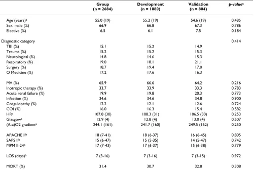
Among 2823 patients, 139 were excluded due to incom-plete or erroneous data (4.9%), leaving 2684 eligible patients. The development group consisted of 1880 patients (70%) and the validation group consisted of 804 (30%).

(4)

Table 2: Demographic characteristics of patients

Group (n = 2684)

Development (n = 1880)

Validation (n = 804)

p-valuec

Age (years)a _{55.0 (19)} _{55.2 (19)} _{54.6 (19)} _0.485

Sex, male (%) 66.9 66.8 67.3 0.786

Elective (%) 6.5 6.1 7.5 0.184

Diagnostic category 0.414

TBI (%) 15.1 15.2 14.9

Trauma (%) 15.2 15.2 15.3

Neurological (%) 14.8 14.6 15.3

Respiratory (%) 19.0 18.1 21.1

Surgery (%) 18.7 19.4 17.0

O Medicine (%) 17.2 17.6 16.3

MV (%) 65.9 66.6 64.2 0.216

Inotropic therapy (%) 33.7 33.9 33.3 0.783

Acute renal failure (%) 19.9 19.8 20.3 0.773

Infection (%) 34.6 34.6 34.8 0.900

Coagulopathy (%) 12.2 12.1 12.6 0.724

COI (%) 16.0 16.3 15.4 0.582

HRa _{107.8 (30)} _{108.3 (31)} _{106.5 (30)} _0.253

Glasgowa _{12.9 (4)} _{12.8 (4)} _{13.0 (4)} _0.507

(A-a)O2 gradienta _{244.1 (161)} _{241.7 (160)} _{249.5 (162)} _0.250

APACHE IIb _{18 (7-41)} _{18 (6-37)} _{16 (6-45)} _0.805

SAPS IIb _{15 (6-47)} _{15 (5-35)} _{14 (5-47)} _0.742

MPM II-24b _{17 (7-43)} _{17 (6-37)} _{15 (6-38)} _0.779

LOS (days)b _{7 (3-16)} _{7 (3-16)} _{7 (3-15)} _0.972

MORT (%) 31.4 30.7 32.8 0.308

TBI: Traumatic brain injury; O Medicine: Other Medical; MV: Mechanical ventilation; A. renal failure: Acute renal failure; COI: Chronic organ insufficiency; HR: Heart rate; (A-a)O2 gradient: Alveolar-arterial oxygen gradient; LOS: Length of stay; MORT: Hospital mortality; (a)_{: Mean (SD);}(b)_: Median (Interquartile range) pc_:_D_{etermined by}χ2 _{test for percentages,}_t_{test for comparison of means or}_Mann-Whitney_{test for comparison of} medians.

Table 3: Outcome trend over the observation period

All 1997 1998 1999 2000 2001 2002 2003 2004 2005 2006 p-valueb

n 2684 176 191 201 223 279 297 303 319 337 358

---MORT (%) 31.4 35.4 33.7 39.1 35.0 28.4 32.9 33.0 28.6 27.7 23.3 0.112

DEV (%) 70.0 70.8 61.7 69.0 70.9 72.4 68.9 75.4 66.8 70.4 72.6 0.146

APACHE IIa ₁₈

(7-41) 21 (7-41)

19 (8-41)

19 (6-34)

17 (6-36)

14 (5-30)

14 (6-30)

15 (6-35)

16 (7-38)

17 (6-36)

15 (7-34)

0.361

SAPS IIa ₁₅

(6-47) 15 (6-47)

17 (5-41)

12 (4-31)

13 (3-35)

13 (4-27)

13 (4-31)

15 (5-39)

17 (6-37)

13 (5-31)

0.415

MPM II-24a ₁₇

(7-43) 17 (7-43)

16 (6-35)

14 (6-29)

16 (6-35)

14 (6-32)

13 (6-34)

18 (6-39)

18 (6-40)

17 (7-36)

14 (6-34)

0.389

MORT: Hospital mortality; DEV: Development set percentage (a)_{: Median (Interquartile range) p}b_:_D_{etermined by}χ2 _{test for percentages or}

(5)

development and the validation groups. Some character-istics are particular to the ICU, such as the low proportion of scheduled patients (6.5%), the prolonged length of stay (median of 7 days) and the high mortality rate (31.4%).

Table 3 shows the evolution (during the 10 years observed) of hospital mortality, the severity scores and the participation percentage in the development set. There are no significant differences (only the evidence that the number of admissions has kept on increasing).

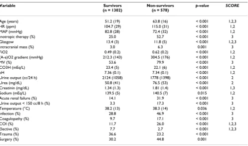
Variable selection: univariate analysis

A total of 24 variables showed significant differences between the survivors and non-survivors (Table 4). The table also shows the scores for which the different varia-bles were included. No significant differences were found for respiratory frequency (APACHE II), serum potassium (APACHE II and SAPS II), hematocrit (APACHE II), leuck-ocyte count (APACHE II y SAPS II), bilirubin (SAPS II), PaO2 (MPM II-24) or antecedents of cirrhosis and neopla-sia (MPM II-24).

Only the COI variable reflected the chronic illnesses of the patient. For variables related to diagnoses, the surgery group was associated with a greater possibility of hospital mortality, while the trauma group was associated with a lower likelihood of mortality.

Multiple Logistic Regression Model

Table 5 shows the LR model including 9 variables (Con-tinuous: Age, HR, Glasgow and (A-a)O2 gradient. Dis-crete: Inotropic therapy, MV, Acute renal failure, COI and Trauma) selected from the 24 variables.

Classification Tree Models

The variables common to the three CTs and the LR model are inotropic therapy (INOT), Glasgow value, (A-a)O2 gradient ((A-a)O2), age and COI.

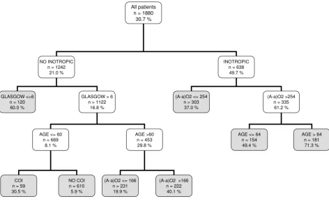
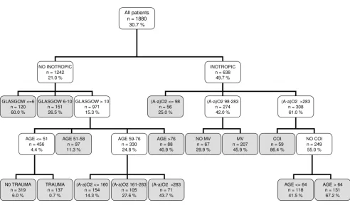
Figure 1 shows the CT based on the CART methodology (the three programs gave the same result). It used only five variables and began with INOT. It generated eight

deci-Table 4: Univariate analyses of characteristics of patients at discharge, by survival status.

Variable Survivors

(n = 1302)

Non-survivors (n = 578)

p-value SCORE

Age (years) 51.2 (19) 63.8 (16) < 0.001 1,2,3

HR (ppm) 104.7 (29) 115.0 (31) < 0.001 1,2

MAP (mmHg) 82.8 (28) 72.4 (32) < 0.001 1,2

Inotropic therapy (%) 25.0 52.7 < 0.001 3

Glasgow 13.4 (3) 11.8 (5) < 0.001 1,2,3

Intracranial mass (%) 3.0 6.3 0.001 3

FiO2 0.49 (0.2) 0.62 (0.2) < 0.001 1,2

(A-a)O2 gradient (mmHg) 212.3 (143) 304.5 (176) < 0.001 1,2

MV (%) 53.6 79.9 < 0.001 3

CO3H (mEq/L) 23.4 (5) 22.1 (6) < 0.001 1,2

pH 7.36 (0.1) 7.34 (0.1) < 0.001 1,2

Urine output (cc/24 h) 2124 (1058) 1778 (1398) < 0.001 2

Urea (mg/dL) 50.8 (41) 76.5 (53) < 0.001 2

Creatinin (mg/dL) 1.34 (1.3) 1.81 (1.4) < 0.001 1,3

Sodium (mEq/L) 139.5 (5) 140.5 (7) 0.015 1,2

Acute renal failure (%) 14.1 31.9 < 0.001 3

Urine output < 150 cc/8 h (%) 3.3 17.3 < 0.001 3

Temperature (°C) 38.2 (13) 38.3 (14) 0.036 1,2

Infection (%) 28.8 46.9 < 0.001 3

Coagulopathy (%) 9.7 17.1 < 0.001 3

COI (%) 11.7 26.0 < 0.001 1,2,3

Elective (%) 7.7 2.7 < 0.001 1,2,3

Trauma (%) 36.6 23.2 < 0.001

Surgery (%) 30.2 44.8 0.001

Development set.

HR: Heart rate; MAP: Mean arterial pressure; (A-a)O2 gradient: Alveolar-arterial oxygen gradient; MV: Mechanical ventilation; COI: Chronic organ insufficiency; MORT: Hospital mortality; Data presented as the mean (SD) or percentages.

SCORE: (1) APACHE II, (2) SAPS II and (3) MPM II 24.

(6)

sion rules with an assignment rank of probability ranging from 5.9% to a maximum of 71.3%.

It is noted that a CT can use the same variables in various decision rules and that, for continuous variables, different cut-off points can be selected.

Figure 2 illustrates the CT based on the CHAID methodol-ogy. It used seven variables, and it also began with the

var-iable INOT. It generated fifteen decision rules with an assignment rank of probability ranging from 0.7% to a maximum of 86.4%. In this type of CT, the Glasgow value, age and (A-a)O2 variables were divided into intervals with more than two possibilities.

Figure 3 depicts the C4.5 model, which used six variables (the five common variables and the MAP, which is not included in the LR model) and generated ten decision

Table 5: Results of multiple logistic regression

Variable Coefficient SD p-value OR 95% CI

Age (years) 0.041 0.004 < 0.001 1.041 1.033 - 1.050

HR (ppm) 0.009 0.002 < 0.001 1.009 1.005 - 1.013

Inotropic therapy 0.730 0.137 < 0.001 2.074 1.585 - 2.714

Glasgow -0.180 0.019 < 0.001 0.835 0.805 - 0.867

MV 0.502 0.145 0.001 1.655 1.245 - 2.201

(A-a)O2 gradient 0.002 0.001 < 0.001 1.002 1.002 - 1.003

Acute renal failure 0.459 0.160 0.002 1.582 1.180 - 2.123

COI 1.026 0.156 < 0.001 2.789 2.054 - 3.788

Trauma -0.357 0.160 0.026 0.700 0.511 - 0.957

Intercept -3.351

HR: Heart rate; MV: Mechanical ventilation; (A-a)O2 gradient: Alveolar-arterial oxygen gradient; COI: Chronic organ insufficiency.

Classification tree by CART algorithm

Figure 1

Classification tree by CART algorithm. The gray squares denote terminal prognostic subgroups. INOT: Inotropic ther-apy; (A-a)O2 gradient: Alveolar-arterial oxygen gradient (mmHg); MV: Mechanical ventilation; COI: Chronic organ insufficiency.

All patients n = 1880

30.7 %

NO INOTROPIC n = 1242

21.0 %

INOTROPIC n = 638 49.7 %

GLASGOW <=6 n = 120 60.0 %

GLASGOW > 6 n = 1122

16.8 %

(A-a)O2 <= 254 n = 303 37.0 %

(A-a)O2 >254 n = 335 61.2 %

AGE <= 60 n = 669

8.1 %

AGE >60 n = 453 29.8 %

AGE <= 64 n = 154

49.4 %

AGE > 64 n = 181

71.3 %

COI n = 59 30.5 %

NO COI n = 610 5.9 %

(A-a)O2 <= 166 n = 231 19.9 %

(7)

rules. The probabilities ranged between 7.6% and 76.2%. In contrast to the other CTs, in this CT, the first variable was the point value on the Glasgow scale.

Comparison of model properties

The three CT models and the LR model were also com-pared with those generated using the APACHE II, SAPS II and MPM II-24 scores.

The severity scores were applied without making recali-bration in all the population (development and valida-tion sets).

Table 6 shows the values for the properties evaluated. It can be seen that all models achieved an acceptable dis-crimination (an AUC greater than 0.70) both in the devel-opment and the validation set.

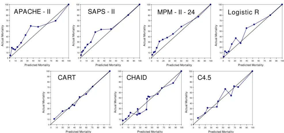
Figure 4 presents the calibration curves of the models. It is notable that some curves were displaced to the observed mortality; this coincided with an SMR greater than 1 (with a CI of 95% that does not include 1) (Table 6). The mod-els based on the CTs were better calibrated (this was observed both in the calibration curves and in the obtained SMR (see Table 6)).

All the models correctly classified approximately 75% of the cases evaluated.

Comparison of individual probabilities generated by the CT models

Table 7 shows the correlations between the probabilities calculated with the 3 CTs and the LR model (all of them statistically significant).

Figure 5 shows the Bland-Altman results obtained in the validation set by comparing the probabilities determined by the CART CT with those of the LR, CHAID and C4.5 CTs.

We observed that there were patients for whom the differ-ence in the probabilities exceeded the acceptable limit of the test. There were 116 patients included in the ison of the CART and CHAID CTs, and 245 in the compar-ison of the CART and C4.5 CTs. The differences can be partly attributed to the behaviour of the Glasgow variable (different cut-off points or partitions) and to the influence of the COI variable in the different divisions of the tree branches.

The different models generate, in some patients, different allocation of death provability. When performing a

vali-Classification tree by CHAID algorithm

Figure 2

Classification tree by CHAID algorithm. The gray squares denote terminal prognostic subgroups. INOT: Inotropic ther-apy; (A-a)O2 gradient: Alveolar-arterial oxygen gradient (mmHg); MV: Mechanical ventilation; COI: Chronic organ insufficiency.

30.7 %

21.0 %

INOTROPIC n = 638

49.7 %

GLASGOW <=6 n = 120 60.0 %

GLASGOW 6-10 n = 151 26.5 %

GLASGOW > 10 n = 971 15.3 %

(A-a)O2 <= 98 n = 56 25.0 %

(A-a)O2 98-283 n = 274 42.0 %

(A-a)O2 >283 n = 308 61.0 %

AGE <= 51 n = 456

4.4 %

AGE 51-58 n = 97 11.3 %

AGE 59-76 n = 330 24.8 %

AGE >76 n = 88 40.9 %

NO MV n = 67 29.9 %

MV n = 207 45.9 %

COI n = 59 86.4 %

NO COI n = 249 55.0 %

N0 TRAUMA n = 319

6.0 %

TRAUMA n = 137

0.7 %

(A-a)O2 <= 160 n = 154 14.3 %

(A-a)O2 161-283 n = 105 27.6 %

(A-a)O2 >283 n = 71 43.7 %

AGE <= 64 n = 118 41.5 %

(8)

dation with records not used in the phase of development, the different allocation of probability determines in our case a conservation of a similar discrimination but that the calibration is different (being better for the AC).

Discussion

The results illustrate that the ICU had particular demo-graphic characteristics due to its case mix, with a low per-centage of scheduled patients, a long length of stay and high mortality. These data are important when it comes to appraising and generalising the results obtained with our database [16].

The results yielded mortality rates that were higher than expected (according to the classic APACHE II, SAPS II and MPM II-24 scores), which can be partly attributed to these individual characteristics [17]. However, this finding also necessitates a recalibration of these models in order to achieve a correct stratification of the patients' risk of hos-pital mortality [18].

Previously, CTs have been used with critical patients, e.g., for the calculation of the probability of death from coro-nary pathology [19], intracerebral haemorrhages [20] or traumatic brain injuries [21], for the prediction of persist-ent vegetative states [22] or (as in our study) for stratifying the probability of death in a general population of ICU patients [23,24].

The common variables selected by the three CT types (and also by the model based on LR) were: the necessity of ino-tropic therapy, the point value on the Glasgow coma scale, the alveolar-arterial gradient in oxygen, age and the pres-ence of antecedents of important chronic diseases. This group of variables included information concerning chronic health and age (which were variables specific to the patient), the point value on the Glasgow coma scale and the (A-a)O2 gradient as deviations from the normal state as well as a variable specific to the intensive treat-ment (INOT). The selection of some of these variables has

Classification tree by C4.5 algorithm

Figure 3

Classification tree by C4.5 algorithm. The gray squares denote terminal prognostic subgroups. INOT: Inotropic therapy; (A-a)O2 gradient: Alveolar-arterial oxygen gradient (mmHg); MV: Mechanical ventilation; COI: Chronic organ insufficiency; MAP: Mean arterial pressure.

30.7 %

GLASGOW <= 5 n = 126

76.2 %

GLASGOW > 5 n = 1754

27.5 %

18.1 %

INOTROPIC n = 581 46.5 %

AGE <= 55 n = 606

7.6 %

AGE > 81 n = 56 63.9 %

COI n = 108

68.5 %

NO COI n = 473 41.4 %

AGE <= 64 n = 216 28.7 %

AGE > 64 n = 257 52.1 % AGE 56-81

n = 531 26.9 %

(A-a)O2 > 231 N = 164

42.0 % (A-a)O2 <= 231

n = 347 19.6 %

MAP > 48 n = 159

23.5 %

MAP <= 48 n = 57 54.1 %

(A-a)O2 <= 301 n = 146

39.7 %

(9)

also been reported in other studies of mortality in other groups of critical patients [25].

These five variables are capable of stratifying the exam-ined population of critical patients (for example, as in the CART CT), using eight simple decision rules, with accept-able properties of discrimination and calibration.

We also observed that the three CT types exhibited differ-ences. Even when incorporating the five common varia-bles mentioned earlier, these CTs differed in the first variable to be selected, in the details of "branching", in the cut-off points (and subgroups), in the order of variable selection and in the incorporation of other variables.

Table 6: Performance of the classification models: development and validation sets

DEVELOPMENT (n = 1880)

Models AUC (CI 95%) HL-C Brier PPV (CI 95%) PCC (CI 95%) SMR (CI 95%)

APACHE II 0.81 (0.79 - 0.83) 68.2 0.17 0.72 (0.66 - 0.78) 0.75 (0.73 - 0.77) 1.30 (1.23 - 1.37) SAPS II 0.82 (0.80 - 0.84) 77.2 0.16 0.74 (0.68 - 0.79) 0.74 (0.68 - 0.75) 1.31 (1.24 - 1.38) MPM II 24 0.81 (0.79 - 0.83) 74.2 0.16 0.75 (0.70 - 0.80) 0.77 (0.75 - 0.79) 1.29 (1.22 - 1.36) Logistic R 0.83 (0.81 - 0.85) 16.8 0.16 0.75 (0.70 - 0.80) 0.77 (0.76 - 0.79) 1.00 (0.92 - 1.10) CART 0.78 (0.76 - 0.80) --- 0.17 0.67 (0.61 - 0.72) 0.75 (0.73 - 0.77) 1.00 (0.94 - 1.06) CHAID 0.80 (0.78 - 0.82) --- 0.16 0.68 (0.63 - 0.73) 0.75 (0.73 - 0.77) 1.00 (0.93 - 1.08) C4.5 0.80 (0.78 - 0.82) --- 0.16 0.69 (0.65 - 0.74) 0.78 (0.76 - 0.80) 1.00 (0.94 - 1.06)

VALIDATION (n = 804)

APACHE II 0.77 (0.74 - 0.81) 74.1 0.18 0.69 (0.60 - 0.70) 0.73 (0.70 - 0.76) 1.36 (1.26 - 1.47) SAPS II 0.79 (0.76 - 0.83) 78.3 0.18 0.71 (0.63 - 0.78) 0.74 (0.71 - 0.77) 1.39 (1.28 - 1.49) MPM II 24 0.79 (0.75 - 0.82) 66.9 0.18 0.71 (0.63 - 0.78) 0.74 (0.71 - 0.77) 1.36 (1.25 - 1.46) Logistic R 0.81 (0.78 - 0.84) 41.5 0.17 0.73 (0.66 - 0.81) 0.75 (0.73 - 0.78) 1.22 (1.16 - 1.29) CART 0.75 (0.71 - 0.81) --- 0.18 0.64 (0.57 - 0.72) 0.72 (0.69 - 0.75) 1.04 (0.95 - 1.31) CHAID 0.76 (0.72 - 0.79) --- 0.18 0.64 (0.56 - 0.72) 0.72 (0.69 - 0.75) 1.06 (0.97 - 1.15) C4.5 0.76 (0.73 - 0.80) --- 0.18 0.70 (0.63 - 0.76) 0.76 (0.73 - 0.79) 1.08 (0.98 - 1.16)

AUC: Area under ROC curve; CI: Confidence interval; HL-C: Hosmer-Lemeshow test C (eight degrees of freedom); Brier: Brier score; PPV: Positive predictive value (cutoff 0.5); PCC: Percentage correctly classified (cutoff 0.5); SMR: Standardized mortality ratio. The severity scores (APACHE II, SAPS II and MPM II 24) were not developed in the development phase and recalibration was not performed.

Calibration curves for the classification models

Figure 4

Calibration curves for the classification models. Validation set.

APACHE - II

SAPS - II

MPM - II - 24

Logistic R

CART

CHAID

C4.5

0 10 20 30 40 50 60 70 80 90 100

Predicted Mortality A c tu a l M o rta lit y 0 10 20 30 40 50 60 70 80 90 100

0 10 20 30 40 50 60 70 80 90 100

(10)

We have already seen that the CART CT includes the five general variables. The C4.5 CT adds the MAP (Mean Arte-rial Pressure) variable and the CHAID CT includes MV (Mechanical Ventilation) variables and the fact of belong-ing to the trauma group. The LR model uses those of the CHAID CT model, also including the Acute Renal Failure and HR (Heart Rate) variables.

The CT software allows to adjust the levels and the number of partitions for each branch in order to get more complex models [7]. In our case, our only restriction (in the 3 CT models) was that the minimum number of sub-jects in the terminal nodes should be of 50 patients.

We cannot state which CT was optimal (since they had similar general properties). The CART and CHAID CTs were similar in their order of partitioning, although the CHAID CT (due to its inherent characteristics) separated the continuous variables into more than two possibilities and generated more decision rules. The CART CT was sim-pler, while the CHAID CT showed greater complexity

(and also selected more variables). Different CTs can select different first variables, and in the C4.5 CT, the first variable, the Glasgow point value, was different from that of the other CTs; the C4.5 CT also incorporated different variables. The analysis of the individual probabilities gen-erated by the different CTs (in spite of a good correlation) assisted in the identification of possible "problem" varia-bles, e.g. the Glasgow point value and the COI variable, in their order of appearance in the decision rules generated.

The CTs most widely used for medical applications have been based on the CART methodology, but studies that use other CT types have started to appear [26-28].

When there is a classification problem, there is no model that can be chosen a priori to be the best [29]. Even with the same information, different CTs develop models with different interpretations [30]. Based on our data, the CTs do not compete with the classic scores in their function of calculating individual probabilities. In the case of a large database, the CTs generated would be too complex to

Table 7: Correlation matrix of the probabilities (CTs and LR models)

DEVELOPMENT SET (n = 1880) VALIDATION SET (n = 804)

LR CART CHAID LR CART CHAID

LR --- --- --- --- ---

---CART 0.872 --- --- 0.877 ---

---CHAID 0.803 0.821 --- 0.788 0.810

---C4.5 0.768 0.796 0.789 0.777 0.794 0.801

LR: Logistic Regression. Numbers represent Spearman correlations coefficients. All values with a p-value < 0.001.

Bland-Altman plot analysis

Figure 5

Bland-Altman plot analysis. (a) CART vs Logistic Regression. (b) CART vs CHAID. (c) CART vs C4.5. The dotted lines are the limits of agreement (mean ± 2 SD). Validation set.

(CART + C4.5) / 2

1,0 ,8 ,6 ,4 ,2 0,0

CA

RT

C

4

.5

1,0

,8

,6

,4

,2

,0

-,2

-,4

-,6

-,8 -1,0

(CART + CHAID) / 2

1,0 ,8 ,6 ,4 ,2 0,0

C

A

RT

CHA

ID

1,0

,8

,6

,4

,2

,0

-,2

-,4

-,6

-,8 -1,0

b

(CART + Logistic R) / 2

1,0 ,8 ,6 ,4 ,2 0,0

CA

RT

L

o

g

is

tic

R

1,0

,8

,6

,4

,2

,0

-,2

-,4

-,6

-,8 -1,0

(11)

interpret and use with regularity (many branches and decision rules). The immediate interpretative advantage of CTs is only obtained with simple trees [31,32].

Our study had several limitations. In the first place, it was carried out in only one ICU and within a ten-year span database (although no variation was observed during the period of study). It would also have been possible to employ more methodologies for comparison or to improve those that were used, by incorporating relations and/or ranks of a priori variables, as do the classic scores.

As exposed by one of the reviewers, we found a great dif-ference between the observed and expected mortality in the validation group in the LR model. The LR-based model could have been carried out using the variables as categorical, thus minimizing the possible effect that out-lier values (using the variables as continuous) have on the predicted outcome. One of the advantages of CT-based models is that they automatically change the continuous variables into categorical ones and that their cut-off points could also be used to create a LR model with discreet var-iables

We must mention the effort at Waikato University (New Zealand) regarding the free-access program WEKA, which strives to collect (in a single tool) the majority of the methodologies that are used to classify, select and group variables [11].

There are models, with different methodologies that could improve the individual properties and achieve greater precision in classification [33,34].

The principal advantage of CTs is that they are easy to interpret. However, this advantage could turn into an obstacle, since we tend to choose the optimal CT as that which more closely approaches the clinical reasoning that coincides with that of the program user [35]. An under-standing of the clinical problem is necessary in order to adequately interpret CTs.

One contribution of our effort was the demonstration that the CT methodology is not unique and that different CTs could be generated according to various methodologies. The CTs assisted in both selecting variables of greater importance in the problem of classification and determin-ing the best cut-off points for the continual variables.

We believe that CTs (e.g., the model based on CART) are mainly useful in obtaining homogenous groups for the assignation of the probability of hospital mortality. These groups with different characteristics (defined by rules of classification that can be interpreted) can serve, for exam-ple, as a basis for the creation of new scores.

We intend to do further research including a multi-centre study, with the incorporation of more methodologies and the possible use of hybrid models. In order to generalise our results, external validation will be required [36].

Conclusion

The main benefits to CT analysis are to identify a relatively small number of groups that are reasonably homogene-ous with regard to the outcome. The CTs can be used in intensive care medicine for assisting in diagnosis and prognosis [37,38]. Those less familiar with CTs should realise that this us a class of methods including many dif-ferent approaches, and that these difdif-ferent approaches may result in considerable differences in classifications.

Competing interests

The authors declare that they have no competing interests.

Authors' contributions

JT and JM provided the CT procedure, implemented the algorithms, performed statistical and drafted the manu-script. MB, LS and ARP analyzed the data, interpreted the results and wrote the final paper. All authors read and approved the final manuscript.

References

1. Lemeshow S, Le Gall JR: Modeling the severity of illness of ICU patients. JAMA 1994, 272:1049-1055.

2. Knaus WA, Draper EA, Wagner DP, Zimmerman JE: APACHE II: A severity of disease classification system. Crit Care Med 1985, 13:818-829.

3. Le Gall JR, Lemeshow S, Saulnier F: A new simplified acute phys-iology score (SAPS II) based on a European/North American multicenter study. JAMA 1993, 270:2957-63.

4. Lemeshow S, Teres D, Klar J, Avrunin JS, Gehlbach SH, Rapoport J: Mortality probability models (MPM II) based on an interna-tional cohort of intensive care unit patients. JAMA 1993, 270:2478-86.

5. Tom E, Schulman KA: Mathematical models in decision analy-sis. Infect Control Hosp Epidemiol 1997, 18:65-73.

6. Harper PR: A review and comparison of classification algo-rithms for medical decision making. Health Policy 2005, 71:315-31.

7. Trujillano J, Sarria-Santamera A, Esquerda A, Badia M, Palma M, March J: Aproximación a la metodología basada en árboles de decisión (CART). Mortalidad hospitalaria del infarto agudo de miocardio. Gac Sanit 2008, 22:65-72.

8. Crichton NJ, Hinde JP, Marchini J: Models for diagnosing chest pain: is CART helpful? Stat Med 1997, 16:717-27.

9. Knaus WA, Wagner DP, Draper EA, Zimmerman JE, Bergner M, Bas-tos PG, et al.: The APACHE III prognostic system. Risk predic-tion of hospital mortality for critically ill hospitalized adults.

Chest 1991, 100:1619-1636.

10. Hosmer DW, Lemeshow S: Applied logistic regression 2nd edition. John Wiley & Sons New York; 2000.

11. Ian H: Witten and Eibe Frank. In Data Mining: Practical machine learning tools and techniques 2nd edition. Morgan Kaufmann, San Fran-cisco; 2005.

12. Hanley JA, McNeil BJ: The meaning and use of the area under a receiver operating characteristic (ROC) curve. Radiology

1982, 143:29-36.

13. Lemeshow S, Hosmer DW: A review of goodness of fit statistics for use in the development of logistic regression models. Am J Epidemiol 1982, 115:92-106.

(12)

Publish with BioMed Central and every scientist can read your work free of charge

"BioMed Central will be the most significant development for disseminating the results of biomedical researc h in our lifetime."

Sir Paul Nurse, Cancer Research UK

Your research papers will be:

available free of charge to the entire biomedical community

peer reviewed and published immediately upon acceptance

cited in PubMed and archived on PubMed Central

yours — you keep the copyright

Submit your manuscript here:

http://www.biomedcentral.com/info/publishing_adv.asp

BioMedcentral

intensive care units: A multicenter inception cohort study.

Crit Care Med 1994, 22:1385-1391.

15. Bland JM, Altman DG: Statistical methods for assessing agree-ment between two methods of clinical measureagree-ment. Lancet

1986, 1:307-10.

16. Trujillano J, March J, Badia M, Rodriguez A, Sorribas A: Aplicación de las Redes Neuronales Artificiales para la estratificación de riesgo de mortalidad hospitalaria. Gac Sanit 2003, 17:504-11. 17. Zimmerman JE, Wagner DP: Prognostic systems in intensive

care: How do you interpret an observed mortality that is higher than expected? Crit Care Med 2000, 28:258-260. 18. Zhu BP, Lemeshow S, Hosmer DW, Klar J, Avrunin JS, Teres D:

Fac-tors affecting the performance of the models in the Mortality Probability Model II system and strategies of customization: A simulation study. Crit Care Med 1996, 24:57-63.

19. Austin PC: A comparison of regression trees, logistic regres-sion, generalized additive models, and multivariate adaptive regression splines for predicting AMI mortality. Stat Med

2007, 26:2937-57.

20. Takahashi O, Cook EF, Nakamura T, Saito J, Ikawa F, Fukui T: Risk stratification for in-hospital mortality in spontaneous intrac-erebral haemorrhage: a Classification and Regression Tree analysis. QJM 2006, 99:743-50.

21. Rovlias A, Kotsou S: Classification and Regression tree for pre-diction of outcome after severe head injury using simple clin-ical and laboratory variables. J Neurotrauma 2004, 21:886-893. 22. Dolce G, Quinteri M, Serra S, Lagani V, Pignolo L: Clinical signs and

early prognosis in vegetative state: a decisional tree, data-minig study. Brain Inj 2008, 22:617-23.

23. Abu-Hanna A, de Keizer N: Integrating classification trees with local logistic regression in Intensive Care prognosis. Artif Intell Med 2003, 29:5-23.

24. Gortzis LG, Sakellaropoulos F, Ilias I, Stamoulis K, Dimopoulou I: Predicting ICU survival: a meta-level approach. BMC Health Serv Res 2008, 26:8-157.

25. de Rooij SE, Abu-Hanna A, Levi M, de Jonge E: Identification of high-risk subgroups in very elderly intensive care unit patients. Crit Care 2007, 11:R33.

26. Gerald LB, Tang S, Bruce F, Redden D, Kimerling ME, Brook N, Dun-lap N, Bailey WC: A decision tree for tuberculosis contact investigation. Am J Respir Crit Care Med 2002, 166:1122-7. 27. Costanza MC, Paccaud F: Binary classification of dyslipidemia

from the waist-to-hip ratio and body mass index: a compari-son of linear, logistic, and CART models. BMC Med Res Meth-odol 2004, 4:7-17.

28. Muller R, Möckel M: Logistic regression and CART in the anal-ysis of multimarker studies. Clin Chim Acta 2008, 394:1-6. 29. Magdon-Ismail M: No free lunch for noise prediction. Neural

Comput 2000, 12:547-64.

30. Wolfe R, McKenzie DP, Black J, Simpson P, Gabbe BJ, Cameron PA: Models developed by three techniques did not achieve acceptable prediction of binary trauma outcomes. J Clin Epi-demiol 2006, 59:26-35.

31. Peters RP, Twisk JW, van Agtmael MA, Groeneveld AB: The role of procalcitonin in a decision tree for prediction of blood-stream infection in febrile patients. Clin Microbiol Infect 2006, 12:1207-13.

32. Mann JJ, Ellis SP, Waternaux CM, Liu X, Oquendo MA, Malone KM, Brodsky BS, Haas GL, Currier D: Classification trees distinguish suicide attempters in major psychiatric disorders: a model of clinical decision making. J Clin Psychiatry 2008, 69:23-31. 33. Pang BC, Kuralmani V, Joshi R, Hongli Y, Lee KK, Ang BT, Li J, Leong

TY, Ng I: Hybrid outcome prediction model for severe trau-matic brain injury. J Neurotrauma 2007, 24:136-46.

34. Gaudart J, Poudiogou B, Ranque S, Doumbo O: Oblique decision trees for spatial pattern detection: optimal algorithm and application to malaria risk. BMC Med Res Methodol 2005, 5:22. 35. Podgorelec V, Kokol P, Stiglic B, Rozman I: Decision trees: an

overview and their use in medicine. J Med Syst 2002, 26:445-63. 36. van Dijk MR, Steyerberg EW, Stenning SP, Habbema JD: Identifying subgroups among poor prognosis patients with nonsemino-matous germ cell cancer by tree modelling: a validation study. Ann Oncol 2004, 15:1400-5.

37. Webster AP, Goodacre S, Walker D, Burke D: How do clinical fea-tures help identify paediatric patients with fracfea-tures follow-ing blunt wrist trauma? Emerg Med J 2006, 23:354-7.

38. Köhne CH, Cunningham D, Di CF, Glimelius B, Blijham G, Aranda E, Scheithauer W, Rougier P, Palmer M, Wils J, Baron B, Pignatti F, Schöffski P, Micheel S, Hecker H: Clinical determinants of sur-vival in patients with 5-fluorouracil-based treatment for metastatic colorectal cancer: results of a multivariate analy-sis of 3825 patients. Ann Oncol 2002, 13:308-17.

Pre-publication history

The pre-publication history for this paper can be accessed here: