MURDOCH RESEARCH REPOSITORY
http://dx.doi.org/10.1109/NNSP.2000.889361
Zaknich, A. and Attikiouzel, Y. (2000) A tunable approximately
piecewise linear model derived from the modified probabilistic
neural network. In: Proceedings of the 2000 IEEE Signal
Processing Society Workshop: Neural Networks for Signal
Processing X, 11 - 13 December, Sydney, Australia, pp. 45-53.
http://researchrepository.murdoch.edu.au/18343/
Copyright © 2000 IEEE
Personal use of this material is permitted. However, permission to reprint/republish
this material for advertising or promotional purposes or for creating new collective
A TUNABLE APPROXIMATELY PIECEWISE
LINEAR MODEL DERIVED FROM THE
MODIFIED PROBABILISTIC NEURAL
NETWORK
Anthony Zaknich and Yianni Attikiouzel
Centre for Intelligent Information Processing Systems (CIIPS), The University of Western Australia, Nedlands 6907, Western Australia
A simple model which can be adjusted by a single smoothing parameter continuously from the best piecewise linear model in each linear subregion to the best approximately piecewise lmear model overall is developed for multivariate general nonlinear regression. The model provides an accurate, smooth approximately piecewise linear model to cover the entire data space. It provides a logical basis for extrapolation to regions not represented by training data, based on the closest piecewise linear model. This model has been developed by making relatively minor changes to the form of the Modified Probabilistic Neural Network, a network used for general nonlinear regression. The Modified Probabilistic Neural Network structure allows it to model data by weighting piecewise linear models associated with each of the network’s radial basis functions in the data space.
1.0
INTRODUCTION
Nonlinear regression, based on a limited set of training data, can have significant limitations. When the underlying function is unknown the regression can, at best, only accurately interpolate within the region of the training inputloutput pairs. Also, there is no guarantee that the regression will be able to adequately extrapolate outside the region of the training data. However, in many practical nonlinear problems the underlying function may be relatively smooth and have many regions that are close to linear. In those cases the function can be modeled with an approximately piecewise linear model. It may therefore be useful to have a simple model which can be adjusted by a single smoothing parameter continuously from the best piecewise linear model in each linear subregion to the best approximately piecewise linear model overall.
This paper introduces a model which defines a multivariate scalar function over the whole data space and which can always be tuned to produce the best approximation in the region of the training data. The assumption is made that in the region where there is no training data it is best to extrapolate based on the closest piecewise linear model determined from the local training data. In the regions covered by training data the model interpolates to provide the most accurate representation of the underlying nonlinear function. As more training
data is acquired the model can be adjusted by adapting the appropriate piecewise linear models to maintain accurate representation in regions where training data does exist. In this way the model is as accurate as it can be within regions covered by training data. Also, the various piecewise linear models provide a
logical basis for extrapolation to regions devoid of training data. This is a sensible strategy if a reasonable amount of representative training data is available in the first instance and if the underlying function is not grossly nonlinear. However, the method can work well for more nonlinear functions as well.
A model as described above can be developed by making relatively minor changes to the form of the Modified Probabilistic Neural Network (MPNN). I n
this case The MPNN structure allows it to be used to model data by the weighted sum of piecewise linear models associated with each of the network’s Radial Basis Functions (RBFs) in the data space. The piecewise linear models associated with each RBF are computed using the same set of data points which are used to determine the RBF centre vector, being the mean of those points.
2.0 REVIEW OF THE MODIFIED PROBABILISTIC
NEURAL NETWORK
The Modified Probabilistic Neural Network was initially introduced by Zaknich et al in 1991 [ 1,2] for application to general signal processing and pattern recogrution problems. It is a generalisation of Specht’s General Regression Neural Network (GRNN) [3] and is related to Specht’s Probabilistic Neural Network (PNN) [4] classifier. The MPNN and GRNN have similarities with the method of
Moody and Darken [ 5 ] ; the method of radial basis functions [ 6 ] ; the Cerebellar Model Articulation Controller (CMAC) [ 7 ] ; and a number of other nonparametric kernel based regression techniques stemming from the work of Nadaraya [SI and Watson [8]. If it can be assumed that for each local region in the input space represented by a centre vector ci there is a corresponding scalar output y, that it maps into then a convenient general model to use for all forms of the MPNN and the GlWN is (I).
.f, (Ilx - ci
11,
U ) is a suitable radial basis function.Ci
Yi
M
z i
0
centre vector for class i in the input space. learning parameter chosen during training. output related to ci (real valued or quantised). number of unique centres ci.
number of vectors x . J associated with centre ci.
M
i=l
N S total number of training vectors ( NS = 2; ).
Equation ( I ) represents the GRNN if all the + I , the y , are real valued, the centre vectors c i are replaced with individual training vectors x i and M=NS. A Gaussian radial basis function is often used for,fi(x) as defined by (2).
Equation (2) can be more conveniently represented in the form defined by (3)
where di = IIx
-till
= d ( x - c, ) T ( x - c , ) ,the Euclidean distance between vectors x and ci
One simple way the MPNN set of training pairs (ci+yi
I
[ = I , ..., M } can be formed is to first partition the input space into uniform hypercubes. Then, make ci to be the mean of all training input vectors, x,, in each hypercube that map to y i . The value y i is computed as the mean of the corresponding outputs y,. These outputs must be sufficiently close to each other to be adequately represented by their mean. In this way a local group of vectors in the input space can be replaced witha single centre vector whch maps to a single mean output value. The value Zi is simply the number of vectors x j averaged to make centre c i . A number of different hypercube sizes can be systematically tested to choose the best one. There is usually a wide range of acceptable hypercube sizes between small and large which can be found easily and relatively quickly.
Training simply involves finding the single optimal learning parameter ( 5 giving
the minimum Mean Squared Error (MSE) of the network output minus the desired output for a representative testing set of known sample vector pairs ( x k + y k
I
k = l , ... NUM}. In most applications there is a unique
o that produces the
minimum MSE between the network output and the desired output for the testing set and can be found quite easily by trial and error. Since the relation between oand MSE is usually smooth with a broad minimal MSE section, o can often be found very quickly by a convergent optimisation algorithm based on recurrent parabolic curve fitting [IO].
3.0 THE NEW LINEAR MPNN MODEL
The new approximately piecewise linear regression model can be formed by first partitioning the input space into uniform hypercubes as is done for the MPNN.
When the centre vectors ci are found use the Zi corresponding input vectors
xi
to create a set of best fit least squares linear regression models associated with each of the centres. The outputs y, in (1) are then replaced with the output of the linear model for all input vectors during operation instead of the previous fixed mean output values of the original M P N N . When this is done the linear model outputs provide much more accurate mappings from the input to the output space than to the means y,. Consequently, the input space hypercubes can be made much larger and fewer (M), resulting in a much smaller network size for comparable accuracy.In this new model the adjustment of
o
during training will control the degree of weighting of each linear model associated with each centre. Input vectors closest to a centre will activate the associated linear model more than for those further away. For very small o the linear model associated with the centre closest to the current input point will dominate, resulting in a linear response in the local space of that centre. For very large o the network output will approach an unweighted biased average of all the linear models. Somewhere in between an optimal model will result which provides linear operation close to each centre and deviating from linearity close to centre boundaries. At the boundaries a smooth merging ofneigbowing linear models occurs.
4.0
EXAMPLE RESULTS
To provide a visual demonstration of the new model’s features and operation a
simple one-dimension nonlinear function regression has been chosen. The model works in a similar fashion for higher dimensional problems with no loss of generality.
A third order polynomial function defined by (4) was used as the underlying reference function from which a set of training and testing vector pairs were derived in the x interval [0,10. I].
The training data was 70 pairs ( x , y ) from (4) for d . 1 to 2.0 at a regular x sampling interval of 0.1 plus x=5.1 to 10.0 also at a regular sampling internal of
0.1. These training data are shown with asterisks in Figure I where it can be seen
that there is a large gap in the x interval [2.1,5.0]. The thin solid line in Figure 1 shows the entire function over the x interval [O. 1, IO] and it represents the desired function output. Two sets of independent test data pairs (x,y) were also constructed. The first set was a 100 pairs from the x interval [0.005,9.995] at a
regular sampling interval of 0.1. This first test set was chosen from in between the training set data to avoid duplication. The second testing set was a 100 pairs spread evenly over the x interval but with uniform zero mean random noise, having a variance of 0.0192, added to the x variable after the y was computed according to (4). The first test set is shown as the smooth curve in Figure 2 and the second noisy set is the other curve.
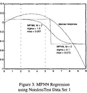
The first test shows how the original MPNN and the new Linear MPNN deal with interpolation between centres for regions devoid of training data. To achieve this a MPNN with M = 2 has been developed using the training data. There are two
RBF centers, one for each set of training data either side of the gap in the x
interval [2.1,5.0]. Figure 3 shows the function approximation for the standard MPNN. When the learning parameter sigma is small the MPNN approximation is a stair step with a discontinuity between the two centres. As sigma is increased to the optimal value of 1.9 there is a smooth connection between the centres and the MSE improves from 0.073 to 0.057.
n z I .: . . ' . . .
1 :
0 6 .
.
. , .. -
I .
. . .
I t ' ' ' ' ' ' ' ' ' 1
0 1 2 3 4 5 6 7 8 9 10
Figure 1: Training Data and Desired Output
0-7803-6278-0/00$10.00 ( C ) IEEE
Figure 2: Testing Data
0 4
0 2
0
0 2
0 4
0 6
0 8
1
0 1 2 3 4 5 6 7 8 9
Figure 3: MPNN Regression using NoislessTest Data Set 1
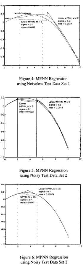
Figure 4 shows the function approximation for the new Linear MPNN. When the learning parameter sigma is small the Linear MPNN approximation consists of two linear sections in the two regions controlled by each centre. There is a
discontinuity between the two linear sections. As sigma is increased to the optimal value of 2.4 a smooth connection is made between the linear sections and the MSE improves from 0.0082 to 0.0034. The function approximation achieved with the Linear MPNN is clearly better than the standard MPNN as can be seen by the MSE reduction by a factor of 16.76.
The r1:maining tests were all conducted with the same training data but with the noisy test data set 2. Figure 5 shows the performance of the Linear MPNN for M
= 5. As before the function approximation improves as sigma is increased from
0.1 to the optimal value of 1.2 with corresponding reduction of the MSE from 0.0022 to 0.0018 respectively. Here we see that as M is increased the choice of the sigma value is less sensitive since the MSE is less affected.
Figure: 6 shows comparative standard and Linear MPNN results for M = 35
respectively. .As M is increased the quality of the approximation is further improved for both networks but the network sizes are also increased. It can be seen from the plots that both networks reduce the effects of random noise as well as provide some interpolation in the x interval gap [2.1,5.0]. Once again the Linear MPNN achieves much better performance than the standard MPNN in terms of better interpolation as well as lower MSE. It can be clearly seen in Figure 6 how the Linear MPNN fills the gap region by extrapolation of the piecewise linear sections immediately to either side of the gap. The two linear extrapolations meet in a relatively smooth join.
Figure 7 shows the standard and Linear MPNN plots of MSE versus sigma for the case of M = 5. This demonstrates some important properties of the Linear MPNN. Firstly, the Linear MPNN produces lower MSEs than the standard MPNN for the same network size. It also has a much lower sensitivity to sigma. There is
a very
wide range of sigma values between about 0.1 and 1.5 which produce very acceptable performance in terms of MSE.' m , r = o M B z '
0 1 2 3 4 5 6 7 8 9 10
Figure 4: MPNN Regression using Noiseless Test Data Set 1
O S
4 6 a I O 12
Figure 5: MPNN Regression using Noisy Test Data Set 2
0 2 1 5 8 1 0
-I 21
Figure 6: MPNN Regression using Noisy Test Data Set 2
0 05
0 045 /
0 04 0 035
0 03. 0 0 2 5 . 0 02 0 0 1 5 0 0 1
o m s .
0
mse w "gn"'
/
MPNN. M = 5 /
/ , , " // /
--.
b, '/'
UmarMPNN. M'~ .___ -.,. -'
,Y
-.
5.0 CONCLUSIONS AND DISCUSSION
This paper has introduced a new development of the MPNN, which provides some significant benefits for nonlinear regression based on a limited set of training data. The new Linear MPNN works in much the same way as the standard MPNN but it is more accurate for comparable network sizes. It is also much less sensitive to the selection of the single learning parameter, sigma. Another significant benefit is that the new Linear MPNN is much better able to extrapolate in regions outside of training data.
In this study a linear model has been chosen to derive the training output values y ,
but there is no reason why a quadratic or higher order polynomial can not be used if there is some reason to justify it. Higher order piecewise polynomial models would be expected to provide even more accuracy. The only drawback is that many more piecewise model parameters must be stored for each centre. This may not really be much of a drawback if it allows a function to be better approximated with much fewer centres, ie. smaller M.
The Linear MPNN can easily be made to be adaptive by simple incremental improvement of the piecewise models for each centre as new data pertaining to that centre becomes available. Another very useful way to exploit this new MPNN structure is to use it to smoothly piece together and merge a set of Multi-Layer Perceptron (MLP) models throughout a data space. This provides a method of
decoupling MLP models such that as data statistics change in a local region only the lwLP related to that region needs to be adapted. Not only does this allow the total model to adapt much faster but it also preserves the training of the unaffected MLPs and helps with the stability-plasticity dilemma.
REFERENCES
[ I ] 2:aknich, Anthony, desilva, Christopher and Attiluouzel, Yianni, "The probabilistic neural network for nonlinear time series analysis",
International Joint Conference on Neural Networks (IJCNN), Singapore, 17-
2 1 st November 199 1, pp. 1530- 1535.
[2] Zaknich, A., "Introduction to the modified probabilistic neural network for general signal processing applications", IEEE Transactions on Signal Processing, Vol. 46, No. 7, July 1998, pp. 1980-1990.
[3] Specht, D. F., "A general regression neural network", IEEE Transactions on Neural Networks, Vol. 2, No. 6, November 1991, pp. 568-576.
[4] Specht, D. F., "Probabilistic neural networks", International Neural Network Society, Neural Networks, Vol 3, 1990, pp. 109-1 18.
[5] Moody, J. and Darken, C., "Fast learning in networks of locally-tuned processing units", Neural Computation, Vol. 1 No. 2, September 1989, pp.
28 1-294.
[6] Powell, M. J. D., "Radial basis functions for multivariate interpolation: A review", Technical ReDort DAMPT 19WNA12, Department of Applied Mathematics and Theoretical Physics, Cambridge University, England, 1985.
[ 7 ] Albus, J. S., "A new approach to manipulator control: the cerebellar model articulation controller (CMAC)", Journal of Dvnamic Systems, Measurement, Control, September, 1975, pp. 220-227.
[8] Nadaraya, E. A., "On estimating regression", Theorv Probability Apolications., 9, 1964, pp. 141-142.
[9] Watson, G. S., "Smooth regression analysis", Sankhva Series A, 26, 1964, pp. 359-372.
[ IOIZaknich, Anthony and Attikiouzel, Yianni, "Automatic optimization of the modified probabilistic neural network for pattern recognition and time series analysis", Proceedings of the First Australian and New Zealand Conference on Intelligent Information Systems, Perth, Western Australia, I-3rd December, 1993, pp. 152-156.