461
Copyright © 2011-15. Vandana Publications. All Rights Reserved.
Volume-5, Issue-3, June-2015
International Journal of Engineering and Management Research
Page Number: 461-466
Improvement in the Kalman Filter in the Modelling of GPS Errors
Viraj1 and Jitender Khurana2 1
Student, M. Tech, SBMNEC, Rohtak, Haryana, INDIA 2
Assistant Professor, ECE, SBMNEC, Rohtak, Haryana, INDIA
ABSTRACT
This paper describes about the modeling of errors (like ionosphericdelays, atmospheric delays, Tropospheric delays, Multipath effects and dilution of precision etc.,) affecting the GPS signals as they travel from satellite to user on Earth. These errors degrade the accuracy of GPS position. An attempt is made to improve the accuracy in locating the GPS receiver by filtering the range measure-ments with the datum conversion between Universal Trans-verse Mercator (UTM) and World Geodetic System (WGS - 84) using single frequency ML-250 hand held GPS receiver and smoothening of these coordinates using Kalman filter. A linear recursive filtering technique, Kalman filter is used for greater accuracy in estimating the position of user by considering the initial state of the system, statistics of sys-tem noise and measurement errors from sensor noise mea-surements. The results of proposed Kalman filter technique give better accuracy with more consistency and are found superior to the standard one.
Keywords----GPS, Datum conversion, Kalman filter, Recursive algorithm, Error covariance, Measurement-noise.
I. INTRODUCTIONOFGLOBAL
POSITIONING SYSTEM
A Satellite-based system Global Positioning System uses a constellation of 24 satellites to giveanaccurate position of user. GPS receivers have been developed to observe signals transmitted by thesaellites and achieve sub-meter accuracy in pointpositioning and a few Centi-meters in relative positioning. GPS can be operated in all weather, day andnightwith outany requirement of Inter visibilitybetween Point. GPS provides a global absolutepositioning capability with respect to a con-sistentterrestrial reference frame and considered as
462
Copyright © 2011-15. Vandana Publications. All Rights Reserved.
et al (2006) have also adapted a technique, which utilizessemi-codeless technique to with the use of dual frequen-cy geodetic quality receiver. Kevin Milton et al (2006) have adopted a technique which utilizes a semi-codeless technique to provide high accuracy GPS measurements and L1-L2 carrier phase measurement for wide-lane ap-plications. The delay of the P code is varied and the sig-nals are cross correlated until a maximum value is reached. When thecross correlation of the L1 and L2 signals is at a peak value, the relative delay between the L1 and L2 signals is proportional to the ionospheric de-lay. The derived ionospheric delay may be accounted for in measurement analysis of the L1 signal to provide for a high precision position solution. (http://
www.google.com /patents? hl=en&lr=&vid=USPAT5903654&id=TkcXAAAAEBA
J&oi=fnd&dq=ionospheric+delays;29TH
A significant mathematical toolbox used for stochastic estimation from noisy sensor measurements is Kalman filter. Kalman filtering is based on linear mean square error filtering (estimation) and it is essentially a set of
mathematical equations that implement a Predictor-corrector type estimator which is optimal. It minimizes the estimated error covariance —when some presumed conditions are met. For the given spectral characteristics of an additive combination of signal and noise, the linear operation on this input combination yields the best (meaning minimum square error) separation of the signal from the noise is to be known.
The distinctive feature of Kalman filter is about the description of its mathematical formulation in terms of state space analysis as per (Bozic, 1999) and its solu-tion is computed recursively. As each update estimate is computed from the previous estimate and the input data, only previous estimate requires storage. The filter is a computational algorithm that processes measurements to deduce a minimum error estimate of the system by utiliz-ing knowledge of the system, measurement dynamics, and statistics of the system, noises measurement errors and initial condition information. It is to improve the quality of datum conversion using this smoothening technique. It also reduces the error while converting from UTM to WGS-84 GPS data. Here by employing this smoothening technique, Kalman filter puts up better UTM to WGS-84 conversion efficiency. The effects of ionospheric delays have already been discussed by Klo-buchar (May 1987). Smoothening of WGS- 84 with the help of Kalman filter has been discussed by Malleswari et al (2005). But in this proposed technique, the Kalman filter is used to smoothen the UTM coordinates. Since the time of its introduction, the Kalman filter has been the subject of extensive research and application, particu-larly in the area of autonomous or assisted navigation. This is likely due in large part to advances in digital computing, relative simplicity and robust nature of the filter itself. Rarely do the conditions simultaneously and determining the positions using all of the available ob-servations with a least – squared – error algorithm.
III. MATHEMATICAL FORMULATION
OF KALMANFILTER
The Kalman filter addresses the general problem of
try-ing to estimate the state DEC 2006).The
GPS receiver is giving both WGS-84 data observed in latitude, longitude & altitude and UTM data observed in Northing & Easting (Langely .R.B, 2000). In the con-version process of UTM to WGS 84, accuracy must be obtained without distortions .In the work attempted by-Ravindhra .et al (Feb, 2002), only the datum conversion from WGS- 84 to UTM and inaccuracy were discussed. The role of the noise in GPS is only at satellite and re-ceiver segments. The modeling of the noise in satellites and receiver segments are discussed by Langely (March 1997).Y. Yuan and J. Ou (2001) developed one robust recurrence technique, based on the efficient combination of single-frequency GPS observations by users and the high-precision differential ionospheric delay corrections from WAAS. For the commonly used GPS wide-area augmentation systems (WAAS) with a grid ionospheric model, the efficient modeling of ionospheric delays in real time, for single-frequency GPS users, is still a cru-cial issue which needs further research. This is particu-larly necessary when differential ionospheric delay cor-rections cannot be broadcast, when users cannot receive them or when there are ionospheric anomalies. Ionos-pheric delays have a severe effect on navigation perfor-mance of single-frequency receivers. A new scheme is-necessary for optimality actually exist, and yet the filter apparently works well for many applications in spite of this situation as emphasized by (Peter S Maybeck, 2001). Langely (October, 2000) discussed about the GPS re-ceivers tracking 8 or more satellitesextended their work further and recent precise point positioning results show decimeter accuracyproposed which can efficiently ad-dress the above problems.
II.
THE KALMAN FILTER
x
∈ℜ
nX
of a discrete-time
con-trolled process that is governed by the linear stochastic difference equation as in equation 1.
K = A X K -1 + B U K + W K -1
(1)
---
With a measurement
x
∈ℜ
mthat is (as stated in equation 2).ZK = HX K +V K --- (2)
463
Copyright © 2011-15. Vandana Publications. All Rights Reserved.
and measurement noise (respectively). They are assumedto be independent (of each other), white, and with normal probability distributions
P (W) – N (0, Q) --- (3)
P (V) – N (0, R) --- (4)
The process noise covariance Q and measure-ment noise covariance R matrices as in equations 3 & 4 might change with each time step or measurement, how-ever here we assume they are constant (Peter S Maybeck (2001).
The n×n matrix A in the difference equation (1) relates the state at the previous time step K-1 to the state at the current step K, in the absence of either a driving function or process noise. Note that in practice A might change with each time step, but here we assume it is con-stant. The n×l matrix B relates the optional control inpu-tu
∈ℜ
lto the state x. The m×n matrix H inthe measure-ment equation (2) relates the state to the measuremeasure-ment ZKxˆ
. In practice H might change with each time step or measurement, but here we assume it is constant. The Kalman filter estimates a process by using a form of feedback control: the filter estimates the process state at some time and then obtains feedback in the form of (noi-sy) measurements. As such, the equations for the Kalman filter fall into two groups: time update equations and measurement updateequations as shown in figure 1. Dis-crete Kalman filter time update equations (5 & 6) are given as
=
Ax
ˆ
-
+
Bu
k k k −1
--- 5 & 6
P
−=
AP
A
T+
Q
k k −1Time update equations project the state and co-variance estimates forward from time step k-1 to step k. A and B are from equation (1), while Q is from is from equation (.3). Initial conditions for the filter are dis-cussed in the earlier references. Discrete Kalman filter measurement update equations (7, 8 & 9) are given be-low.
K
k=
P
−H
T(
HP
−H
T+
R
)
−1K k
x
ˆ
=
x
−+
K
(
Z
k−
Hx
ˆ
−)---7, 8 & 9
k K k k
P
=
(
I
−
K
H
)
P
− k K kThe time update equations are responsible for projecting forward (in time) the current state and error covariance estimates to obtain the a priori estimates for the next time step. The measurement update equations are responsible for the feedback--i.e. for incorporating a new measurement into the a priori estimate to obtain an improved a posteriori estimate. The time update
equa-tions can also be thought of as predictor equaequa-tions, while the measurement update equations can be thought of as corrector equations. Indeed the final estimation algorithm resembles that of a predictor-corrector algorithm for solving numerical problems.The first task during the measurement update is to compute the Kalman gain, Kk.
The next step is to actually measure the process to obtain Zk, and then to generate an a posteriori state estimate by
incorporating the measurement as in equation (8). The final step is to obtain an aposteriorierror covariance es-timate via equation(9). After each time and measurement update pair, the process is repeated with the previous aposterioriestimates used to project or predictthe new a priori estimates. This recursive nature is one of the very appealing features of the Kalman filter—it makes prac-tical implementations much more feasible than (for ex-ample) an implementation of a Wiener filter (Brown and Hwang 1992) which is designed to operate on all of the data directly for each estimate. The Kalman filter instead recursively conditions the current estimate on all of the past measurements. Figure 1 below offers a complete picture of the operation of the filter, combining the high-level equations 5 & 6.
IV.FILTER PARAMETERS AND TUNING
464
Copyright © 2011-15. Vandana Publications. All Rights Reserved.
Figure1. A complete picture of the operation of theKal-man filter
In closing we note that under conditions where Q and R are in fact constant, both the estimation error covariance PK and the Kalman gain KK will stabilize quickly and then remain constant. If this is the case, these parameters can be pre-computed by either running the filter off-line, or for example by determining the steady-state value of PK It is frequently the case however that the measurement error (in particular) does not re-main constant. For example, when sighting beacons in our optoelectronic tracker ceiling panels, the noise in measurements of nearby beacons will be smaller than that in far-away beacons. Also, the process noise Q is sometimes changed dynamically during filter operation – becoming Qk- in order to adjust to different dynamics.
For example, in the case of tracking the head of a user of a 3D virtual environment we might reduce the magnitude of Qk if the user seems to be moving slowly, and in-crease the magnitude if the dynamics start changing ra-pidly. In such cases Qk
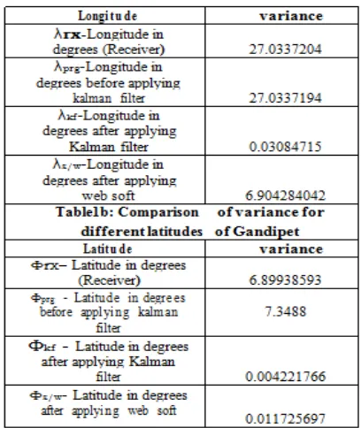
Using single frequency ML 250 GPS hand held receiver, the field data is collected at different Locations in around HussainSagar and Gandipet, Hyderabad. The receiver is giving WGS – 84 data (Ørx and λrx) and UTM data (Nrx&Erx). The variance for WGS 84 of Gandipet is:
λrx-Longitude of Receiver is 27.0337204 in degrees and
Φrx– Latitude of Receiver is 6.89938593 in degrees.The
variance for WGS 84 of HussainSagaris:λrx- Longitude
of Receiver is 13.39910013 in degrees and Φrx– Latitude
of Receiver is 0.020659696 in degrees. Now the UTM coordinates are converted into WGS- 84 coordinates. It is quite evident that the converted values of latitude and longitude (Øprg and λprg) with out applying Kalman filter are giving poor resolution as shown in tables 1and 2. And they are more inconsistent as the variance is more
for the converted data, i.e., Φ
might be chosen to account for both uncertainties about the user's intentions and uncer-tainty in the model.
V. RESULTS AND DISCUSSIONS
prg - Latitude in degrees
before applying kalman filter: 7.3488 (Gandipet) and 0.001264126 (HussainSagar) Hence the UTM data to WGS 84 converted data now smoothened by Kalman filtering algorithm to test the accuracy and consistency (Økf and λ kf) which is giving a very small variance. It is
shown from the tables 1 and 2 that, Φkf – the Latitude in
degrees after applying kalman filter is 0.004221766 for Gandipet and 0.00003667424 for HussainSagar.. Simi-larly, λkf
filter is 0.03084715 for Gandipet and 0.0006331302 for HussainSagar. So, lesser the variance more will be the consistency. Again, the same GPS receiver’s UTM data (Nrx&Erx) is fed to Web Software “Coordinate. Trans-form” to validate WGS 84 data, i.e., (Øs/w &λs/w). This
converted data is also again analyzed asΦ
- Longitude in degrees after applying kalman
s/w- Latitude in degrees after applying websoft is 0.011725697 for Gan-dipet and0.000198005 for HussainSagar. After compar-ing all the variances, that is ( Øs/w, Ørx, Økf&Øprg and
λs/w, λprg, λkf&λrx), it is found that the smoothened
converted data, which is developed from Kalman
filter-ing technique (λkf&Økf), is having better consistency. A
465
Copyright © 2011-15. Vandana Publications. All Rights Reserved.
VI.
CONCLUSION
A comparison of accuracy is suggest-ing,accuracythroughKalman filter application is certainly yielding better results. The present study & data analysis methodology showed that the variations in the signal related to WGS- 84 data can be smoothened using Kalman filter with in the range of studies made and the analysis is found to yield better accuracies as, it is shown from the tables 1 and 2 that, the consistency. However the extensive application of the methodology for the data in bringing out the limitations of the smoothening of the signal, a statistical evaluation atleast in robust domain could throw some light on actual information content & loss of the information through Kalman filteringΦkf – the Latitude in degrees after applying kalman filter is 0.004221766 for Gandipet and 0.00003667424 for
Hus-sainSagar. Similarly, λkf - Longitude in degrees after
466
Copyright © 2011-15. Vandana Publications. All Rights Reserved.
REFERENCES
[1] Bozic.S, M, (1999), Digital and Kalman Filtering: An Introduction to Discrete-Time Filtering and Optimum Linear Estimation, 2nd edition (New York: John Wiley& Sons).
[2] Beran T, S.B. Bisnath and Lagely (2001), Single re-ceiver GPS positioning in support of Airborne gravity for exploration and mapping, Geoide, Fredenton, June 20-22, 2001.
[3]Bisnath S.B and Lagely (2002), High
Precision Kinematic Positioning with a
single GPS Receiver, Navigation; Journal of
the institute Navigation ,vol 49, No 3, Fall 2002 161 – 169.
[4] Brown. R. G. and P. Y. C. Hwang. Introduction to Random Signals and Applied Kalman Filtering, 2nd Edi-tion, John Wiley & Sons, Inc, 1992.
[5] Grewel.M. M S, Lawrence R. Weill, Angus P. An-drews, (2001), Global Positioning System,
Inertial Navigation and Integration, 1st edition (New York: John Wiley & Sons).
[6] Hofmann-Wellenhof, H.Lichteneegger, J.Collins, (1998), Global Positioning Systems: Theory &Practice, 4th edition, (New York/Berlin: Springer-Verlag Wien). [7] Kaplan E (ed), (1996), Understanding GPS: Prin-ciples and Applications, 1st edition (Boston: Artech House).
[8] Kevin Milton et al (Dec, 2006), “Method and appara-tus for eliminating ionospheric delay error in global
posi-tioning system signals” http://www.google.com/patents?hl=en&lr=&v
id=USPAT5903654&id=TkcXAAAAEBAJ&oi=fnd&dq =ionospheric+delays.
[9] Klobuchur J.A (May 1987), “Ionosphere time delay model for single frequency GPS users” ,IEEE Trans Aerospace Electron system (USA).
[10] Langely R.B (March 1997), “The GPS Errorbudget” in GPS world.
[11] Langely.R.B, (2000), “The UTM Grid System, 2nd
[14] Malleswari B.L, MuraliKrishna I.V and LalKishore
K (Jan 2007) “Kalman filter for GPS Datum conver-sion”, Mapworld Forum, Hyderabad.
Ed, (New York: John Wiley & Sons).
[12] Langely R.B (October 2000) “Basic Navigation with a GPS Receiver” GPS World.
[13] Leick.A, (1995), GPS Satellite Surveying, 2nd edi-tion (New York: John Wiley &Sons).
[15] Parkinson, B.W and spilker, J.J (eds), (1996), Glob-al Positioning System: Theory and applications, Volume .1(694pp), Volume 2(632pp), I edition (American Insti-tute of Aeronautics & Astronautics, Inc).
[16] Peter S Maybeck, (2001), Stochastic Models– esti-mation and control, 1st Ed, (New York:PTH).
[17] PratapMisra and Per Enge, (2001), Global Position-ing System Signals, Measurements, and Performance, 1st edition (Massachusetts: Ganga-Jamuna Press).
[18] Ravindhra K, Malleswari B.L. and Sarma A.D (Feb, 2002), “Development of conversion Parameters for GPS Datum”, Proceedings of National conference on GIS and their applications in Civil Engg, Deccan College of Engg, Hyderabad.
[19] Yuan and J.Ou (August, 2001), An improvement to ionospheric delay correction for single-frequency GPS
users - the APR-I scheme, Journal of Geodesy, Volume
75, Numbers 5-6 / , 331-336.