Active Learning for Cost-Sensitive Classification
Akshay Krishnamurthy [email protected]
Microsoft Research New York, NY 10011
Alekh Agarwal [email protected]
Microsoft Research Redmond, WA 98052
Tzu-Kuo Huang [email protected]
Uber Advanced Technology Center Pittsburgh, PA 15201
Hal Daum´e III [email protected]
Microsoft Research New York, NY 10011
John Langford [email protected]
Microsoft Research New York, NY 10011
Editor:Sanjoy Dasgupta
Abstract
We design an active learning algorithm for cost-sensitive multiclass classification: problems where different errors have different costs. Our algorithm, COAL, makes predictions by regressing to each label’s cost and predicting the smallest. On a new example, it uses a set of regressors that perform well on past data to estimate possible costs for each label. It queries only the labels thatcould bethe best, ignoring the sure losers. We proveCOALcan be efficiently implemented for any regression family that admits squared loss optimization; it also enjoys strong guarantees with respect to predictive performance and labeling effort. We empirically compareCOAL to passive learning and several active learning baselines, showing significant improvements in labeling effort and test cost on real-world datasets. Keywords: Active Learning, Cost-sensitive Learning, Structured Prediction, Statistical Learning Theory, Oracle-based Algorithms.
1. Introduction
The field of active learning studies how to efficiently elicit relevant information so learning algorithms can make good decisions. Almost all active learning algorithms are designed for binary classification problems, leading to the natural question: How can active learning address more complex prediction problems? Multiclass and importance-weighted classifi-cation require only minor modificlassifi-cations but we know of no active learning algorithms that enjoy theoretical guarantees for more complex problems.
One such problem is cost-sensitive multiclass classification (CSMC). In CSMC with K classes, passive learners receive input examples x and cost vectors c ∈ RK, where c(y) is
c
the cost of predicting label y on x.1 A natural design for an active CSMC learner then is to adaptively query the costs of only a (possibly empty) subset of labels on each x. Since measuring label complexity is more nuanced in CSMC (e.g., is it more expensive to query three costs on a single example or one cost on three examples?), we track both the number of examples for which at least one cost is queried, along with the total number of cost queries issued. The first corresponds to a fixed human effort for inspecting the example. The second captures the additional effort for judging the cost of each prediction, which depends on the number of labels queried. (By querying a label, we mean querying the cost of predicting that label given an example.)
In this setup, we develop a new active learning algorithm for CSMC called Cost Over-lapped Active Learning (COAL). COAL assumes access to a set of regression functions, and, when processing an example x, it uses the functions with good past performance to compute the range of possible costs that each label might take. Naturally, COAL only queries labels with large cost range, akin to uncertainty-based approaches in active regres-sion (Castro et al., 2005), but furthermore, it only queries labels that could possibly have the smallest cost, avoiding the uncertain, but surely suboptimal labels. The key algorith-mic innovation is an efficient way to compute the cost range realized by good regressors. This computation, andCOALas a whole, only requires that the regression functions admit efficient squared loss optimization, in contrast with prior algorithms that require 0/1 loss optimization (Beygelzimer et al., 2009; Hanneke, 2014).
Among our results, we prove that when processing n (unlabeled) examples with K classes and a regression class with pseudo-dimension d(See Definition 1),
1. The algorithm needs to solve O(Kn5) regression problems over the function class (Corollary 4). ThusCOAL runs in polynomial time for convex regression sets.
2. With no assumptions on the noise in the problem, the algorithm achieves general-ization error ˜O(pKd/n) and requests ˜O(nθ2
√
Kd) costs from ˜O(nθ1 √
Kd) examples (Theorems 5 and 9) whereθ1, θ2 are the disagreement coefficients (Definition 8)2. The worst case offers minimal improvement over passive learning, akin to active learning for binary classification.
3. With a Massart-type noise assumption (Assumption 3), the algorithm has generaliza-tion error ˜O(Kd/n) while requesting ˜O(Kd(θ2+Kθ1) logn) labels from ˜O(Kdθ1logn) examples (Corollary 6, Theorem 10). Thus under favorable conditions, COAL re-quests exponentially fewer labels than passive learning.
We also derive generalization and label complexity bounds under a milder Tsybakov-type noise condition (Assumption 4). Existing lower bounds from binary classification (Hanneke, 2014) suggest that our results are optimal in their dependence on n, although these lower bounds do not directly apply to our setting. We also discuss some intuitive examples highlighting the benefits of using COAL.
CSMC provides a more expressive language for success and failure than multiclass clas-sification, which allows learning algorithms to make the trade-offs necessary for good per-formance and broadens potential applications. For example, CSMC can naturally express
216 218 220 222 224 226 Number of Queries 0.04
0.06 0.08 0.10 0.12 0.14
Test Cost
RCV1-v2 Passive COAL (1e-1) COAL (1e-2) COAL (1e-3)
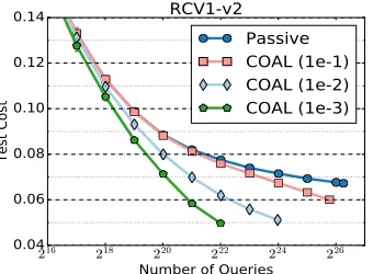
Figure 1: Empirical evaluation of COAL on Reuters text categorization dataset. Active learning achievesbetter test cost than passive, with a factor of 16 fewer queries. See Section 7 for details.
partial failure in hierarchical classification (Silla Jr. and Freitas, 2011). Experimentally, we show thatCOALsubstantially outperforms the passive learning baseline with orders of magnitude savings in the labeling effort on a number of hierarchical classification datasets (see Figure 1 for comparison between passive learning and COALon Reuters text catego-rization).
CSMC also forms the basis of learning to avoid cascading failures in joint prediction tasks like structured prediction and reinforcement learning (Daum´e III et al., 2009; Ross and Bagnell, 2014; Chang et al., 2015). As our second application, we consider learning to search algorithms for joint or structured prediction, which operate by a reduction to CSMC. In this reduction, evaluating the cost of a class often involves a computationally expensive “roll-out,” so using an active learning algorithm inside such a passive joint prediction method can lead to significant computational savings. We show that using COAL within the Aggravatealgorithm (Ross and Bagnell, 2014; Chang et al., 2015) reduces the number of roll-outs by a factor of 14 to 34 on several joint prediction tasks.
Our code is publicly available as part of the Vowpal Wabbit machine learning library.3
2. Related Work
Active learning is a thriving research area with many theoretical and empirical studies. We recommend the survey of Settles (2012) for an overview of more empirical research. We focus here on theoretical results.
Our work falls into the framework of disagreement-based active learning, which studies general hypothesis spaces typically in an agnostic setup (see Hanneke (2014) for an excellent survey). Existing results study binary classification, while our work generalizes to CSMC, assuming that we can accurately predict costs using regression functions from our class. One difference that is natural for CSMC is that our query rule checks the range of predicted costs for a label.
The other main difference is that we use a square loss oracle to search the version space. In contrast, prior work either explicitly enumerates the version space (Balcan et al., 2006;
Zhang and Chaudhuri, 2014) or uses a 0/1 lossclassificationoracle for the search (Dasgupta et al., 2007; Beygelzimer et al., 2009, 2010; Huang et al., 2015). In most instantiations, the oracle solves an NP-hard problem and so does not directly lead to an efficient algorithm, although practical implementations using heuristics are still quite effective. Our approach instead uses a squared-lossregression oracle, which can be implemented efficiently via con-vex optimization and leads to a polynomial time algorithm.
In addition to disagreement-based approaches, much research has focused on plug-in rules for active learning in binary classification, where one estimates the class-conditional regression function (Castro and Nowak, 2008; Minsker, 2012; Hanneke and Yang, 2012; Car-pentier et al., 2017). Apart from Hanneke and Yang (2012), these works make smoothness assumptions and have a nonparametric flavor. Instead, Hanneke and Yang (2012) assume a calibrated surrogate loss and abstract realizable function class, which is more similar to our setting. While the details vary, our work and these prior results employ the same algo-rithmic recipe of maintaining an implicit version space and querying in a suitably-defined disagreement region. Our work has two notable differences: (1) our algorithm operates in an oracle computational model, only accessing the function class through square loss minimization problems, (2) our results apply to general CSMC, which exhibit significant differences from binary classification. See Subsection 6.1 for further discussion.
Focusing on linear representations, Balcan et al. (2007); Balcan and Long (2013) study active learning with distributional assumptions, while the selective sampling framework from the online learning community considers adversarial assumptions (Cavallanti et al., 2011; Dekel et al., 2010; Orabona and Cesa-Bianchi, 2011; Agarwal, 2013). These methods use query strategies that are specialized to linear representations and do not naturally generalize to other hypothesis classes.
Supervised learning oracles that solve NP-hard optimization problems in the worst case have been used in other problems including contextual bandits (Agarwal et al., 2014; Syrgka-nis et al., 2016) and structured prediction (Daum´e III et al., 2009). Thus we hope that our work can inspire new algorithms for these settings as well.
Lastly, we mention that square loss regression has been used to estimate costs for passive CSMC (Langford and Beygelzimer, 2005), but, to our knowledge, using a square loss oracle for active CSMC is new.
Advances over Krishnamurthy et al. (2017). Active learning for CSMC was intro-duced recently in Krishnamurthy et al. (2017) with an algorithm that also uses cost ranges to decide where to query. They compute cost ranges by using the regression oracle to per-form a binary search for the maximum and minimum costs, but this computation results in a sub-optimal label complexity bound. We resolve this sub-optimality with a novel cost range computation that is inspired by the multiplicative weights technique for solving linear programs. This algorithmic improvement also requires a significantly more sophisticated statistical analysis for which we derive a novel uniform Freedman-type inequality for classes with bounded pseudo-dimension. This result may be of independent interest.
general-ization and label complexity bounds for our algorithm in a setting inspired by Tsybakov’s low noise condition (Mammen and Tsybakov, 1999; Tsybakov, 2004).
Comparison with Foster et al. (2018). In a follow-up to the present paper, Foster et al. (2018) build on our work with a regression-based approach for contextual bandit learning, a problem that bears some similarities to active learning for CSMC. The results are incomparable due to the differences in setting, but it is worth discussing their techniques. As in our paper, Foster et al. (2018) maintain an implicit version space and compute maximum and minimum costs for each label, which they use to make predictions. They resolve the sub-optimality in Krishnamurthy et al. (2017) with epoching, which enables a simpler cost range computation than our multiplicative weights approach. However, epoching incurs an additional log(n) factor in the label complexity, and under low-noise conditions where the overall bound isO(polylog(n)), this yields a polynomially worse guarantee than ours.
3. Problem Setting and Notation
We study cost-sensitive multiclass classification (CSMC) problems with K classes, where there is an instance spaceX, a label spaceY ={1, . . . , K}, and a distributionDsupported on X ×[0,1]K.4 If (x, c) ∼ D, we refer to c as the cost-vector, where c(y) is the cost of predictingy∈ Y. A classifier h:X → Y has expected costE(x,c)∼D[c(h(x))] and we aim to find a classifier with minimal expected cost.
Let G,{g:X 7→[0,1]}denote a set of base regressors and let F ,GK denote a set of vector regressors where theythcoordinate off ∈ F is written asf(·;y). The set of classifiers under consideration isH,{hf |f ∈ F }where eachf defines a classifierhf :X 7→ Y by
hf(x),argmin y
f(x;y). (1)
When using a set of regression functions for a classification task, it is natural to assume that the expected costs underDcan be predicted by some function in the set. This motivates the following realizability assumption.
Assumption 1 (Realizability) Define the Bayes-optimal regressorf?, which hasf?(x;y), Ec[c(y)|x],∀x∈ X (with D(x)>0),y∈ Y. We assume that f?∈ F.
While f? is always well defined, note that the cost itself may be noisy. In comparison with our assumption, the existence of a zero-cost classifier inH(which is often assumed in active learning) is stronger, while the existence ofhf? inH is weaker but has not been leveraged
in active learning.
We also require assumptions on the complexity of the classGfor our statistical analysis. To this end, we assume that G is a compact convex subset of L∞(X) with finite pseudo-dimension, which is a natural extension of VC-dimension for real-valued predictors.
Definition 1 (Pseudo-dimension) The pseudo-dimension Pdim(F) of a function class F :X →Ris defined as the VC-dimension of the set of threshold functionsH+,{(x, ξ)7→ 1{f(x)> ξ}:f ∈ F } ⊂ X ×R→ {0,1}.
Assumption 2 We assume thatG is a compact convex set with Pdim(G) =d <∞.
As an example, linear functions in some basis representation, e.g., g(x) = Pd
i=1wiφi(x), where weightswi are bounded in some norm, have pseudodimension d. In fact, our result can be stated entirely in terms of covering numbers, and we translate to pseudo-dimension using the fact that such classes have “parametric” covering numbers of the form (1/ε)d. Thus, our results extend to classes with “nonparametric” growth rates as well (e.g., Holder-smooth functions), although we focus on the parametric case for simplicity. Note that this is a significant departure from Krishnamurthy et al. (2017), which assumed thatG was finite. Our assumption that G is a compact convex set introduces a computational challenging of managing this infinitely large set. To address this challenge, we follow the trend in active learning of leveraging existing algorithmic research on supervised learning (Dasgupta et al., 2007; Beygelzimer et al., 2010, 2009) and access G exclusively through a regression oracle. Given an importance-weighted dataset D ={xi, ci, wi}ni=1 where xi ∈ X, ci ∈R, wi ∈R+, the regression oracle computes
Oracle(D)∈argmin
g∈G
n
X
i=1
wi(g(xi)−ci)2. (2)
Since we assume thatGis a compact convex set it is amenable to standard convex optimiza-tion techniques, so this imposes no addioptimiza-tional restricoptimiza-tion. However, in the special case of linear functions, this optimization is just least squares and can be computed in closed form. Note that this is fundamentally different from prior works that use a 0/1-loss minimization oracle (Dasgupta et al., 2007; Beygelzimer et al., 2010, 2009), which involves an NP-hard optimization in most cases of interest.
Remark 2 Our assumption that G is convex is only for computational tractability, as it is crucial in the efficient implementation of our query strategy, but is not required for our generalization and label complexity bounds. Unfortunately recent guarantees for learning with non-convex classes (Liang et al., 2015; Rakhlin et al., 2017) do not immediately yield efficient active learning strategies. Note also that Krishnamurthy et al. (2017) obtain an efficient algorithm without convexity, but this yields a suboptimal label complexity guarantee.
Given a set of examples and queried costs, we often restrict attention to regression functions that predict these costs well and assess the uncertainty in their predictions given a new example x. For a subset of regressorsG ⊂ G, we measure uncertainty over possible cost values for xwith
γ(x, G),c+(x, G)−c−(x, G), c+(x, G),max
g∈Gg(x), c−(x, G),ming∈Gg(x). (3)
For vector regressors F ⊂ F, we define thecost range for a label y given x asγ(x, y, F),
γ(x, GF(y)) where GF(y) , {f(·;y) | f ∈ F} are the base regressors induced by F for y. Note that since we are assuming realizability, wheneverf? ∈F, the quantitiesc+(x, GF(y)) and c−(x, GF(y)) provide valid upper and lower bounds onE[c(y)|x].
Algorithm 1 Cost Overlapped Active Learning (COAL) 1: Input: Regressors G, failure probability δ≤1/e. 2: Setψi= 1/
√
i,κ= 3, νn= 324(dlog(n) + log(8Ke(d+ 1)n2/δ)). 3: Set ∆i=κmin{iν−1n,1}.
4: fori= 1,2, . . . , n do
5: gi,y ←arg ming∈GRbi(g;y). (See (5)).
6: Define fi ← {gi,y}Ky=1.
7: (Implicitly define) Gi(y)← {g∈ Gi−1(y)|Rbi(g;y)≤Rbi(gi,y;y) + ∆i}.
8: Receive new examplex. Qi(y)←0,∀y∈ Y. 9: for everyy∈ Y do
10: cc+(y)←MaxCost((x, y), ψi/4) andcc−(y)←MinCost((x, y), ψi/4).
11: end for
12: Y0← {y∈ Y |cc−(y)≤miny0
c
c+(y0)}. 13: if |Y0|>1then
14: Qi(y)←1 ify ∈Y0 and cc+(y)−cc−(y)> ψi.
15: end if
16: Query costs of each y withQi(y) = 1. 17: end for
where the editorial effort for inspecting an example is high but each cost requires minimal further effort, as well as those where each cost requires substantial effort. Formally, we define Qi(y) ∈ {0,1} to be the indicator that the algorithm queries label y on the ith example and measure
L1 ,
n
X
i=1
_
y
Qi(y), and L2 ,
n
X
i=1
X
y
Qi(y). (4)
4. Cost Overlapped Active Learning
The pseudocode for our algorithm, Cost Overlapped Active Learning (COAL), is given in Algorithm 1. Given an example x, COAL queries the costs of some of the labels y forx. These costs are chosen by (1) computing a set of good regression functions based on the past data (i.e., the version space), (2) computing the range of predictions achievable by these functions for each y, and (3) querying each y that could be the best label and has substantial uncertainty. We now detail each step.
To compute an approximate version space we first find the regression function that minimizes the empirical risk for each label y, which at roundiis:
b
Ri(g;y), 1 i−1
i−1
X
j=1
(g(xj)−cj(y))2Qj(y). (5)
tolerance on this regret is ∆i at roundi, which scales like ˜O(d/i), where recall thatdis the pseudo-dimension of the classG.
COALthen computes the maximum and minimum costs predicted by the version space Gi(y) on the new example x. Since the true expected cost is f?(x;y) and, as we will see, f?(·;y)∈ Gi(y), these quantities serve as a confidence bound for this value. The computation is done by the MaxCost and MinCost subroutines which produce approximations to
c+(x,Gi(y)) andc−(x,Gi(y)) respectively (See (3)).
Finally, using the predicted costs, COALissues (possibly zero) queries. The algorithm queries anynon-dominated label that has a largecost range, where a label is non-dominated if its estimated minimum cost is smaller than the smallest maximum cost (among all other labels) and the cost range is the difference between the label’s estimated maximum and minimum costs.
Intuitively, COALqueries the cost of every label which cannot be ruled out as having the smallest cost onx, but only if there is sufficient ambiguity about the actual value of the cost. The idea is that labels with little disagreement do not provide much information for further reducing the version space, since by construction all regressors would suffer similar square loss. Moreover, only the labels that could be the best need to be queried at all, since the cost-sensitive performance of a hypothesishf depends only on the label that it predicts. Hence, labels that are dominated or have small cost range need not be queried.
Similar query strategies have been used in prior works on binary and multiclass classifi-cation (Orabona and Cesa-Bianchi, 2011; Dekel et al., 2010; Agarwal, 2013), but specialized to linear representations. The key advantage of the linear case is that the set Gi(y) (for-mally, a different set with similar properties) along with the maximum and minimum costs have closed form expressions, so that the algorithms are easily implemented. However, with a general setGand a regression oracle, computing these confidence intervals is less straight-forward. We use the MaxCostand MinCost subroutines, and discuss this aspect of our algorithm next.
4.1. Efficient Computation of Cost Range
In this section, we describe the MaxCost subroutine which uses the regression oracle to approximate the maximum cost on labelyrealized byGi(y), as defined in (3). The minimum cost computation requires only minor modifications that we discuss at the end of the section. Describing the algorithm requires some additional notation. Let ˜∆j ,∆j+Rbj(gj,y;y)
be the right hand side of the constraint defining the version space at roundj, wheregj,y is the ERM at round j for label y, Rbj(·;y) is the risk functional, and ∆j is the radius used
inCOAL. Note that this quantity can be efficiently computed since gj,y can be found with a single oracle call. Due to the requirement that g ∈ Gi−1(y) in the definition of Gi(y), an equivalent representation is Gi(y) = Ti
j=1{g : Rbj(g;y) ≤ ∆˜j}. Our approach is based
on the observation that given an example x and a label y at round i, finding a function g∈ Gi(y) which predicts the maximum cost for the label yon xis equivalent to solving the minimization problem:
Algorithm 2 MaxCost
1: Input: (x, y), tolerancetol, (implicitly) risk functionals{Rbj(·;y)}ij=1.
2: Compute gj,y= argming∈GRbj(g;y) for eachj.
3: Let ∆j =κmin{jν−1n ,1}, ˜∆j =Rbj(gj,y;y) + ∆j for each j.
4: Initialize parameters: c`←0, ch←1, T ← log(i+1)(12/∆i) 2
tol4 , η←
p
log(i+ 1)/T. 5: while|c`−ch|>tol2/2 do
6: c← ch−c` 2 7: µ(1) ←1∈
Ri+1. .Use MW to check feasibility of Program (9). 8: for t= 1, . . . , T do
9: Use the regression oracle to find
gt←argmin g∈G
µ(0t)(g(x)−1)2+ i
X
j=1
µ(jt)Rbj(g;y) (6)
10: If the objective in (6) forgt is at least µ(0t)c+
Pi
j=1µ (t)
j ∆˜j,c` ←c, go to 5.
11: Update
µ(jt+1)←µ(jt) 1−η∆˜j−Rbj(gt;y) ∆j+ 1
!
, µ(0t+1) ←µ(0t)
1−ηc−(gt(x)−1)
2 2
.
12: end for 13: ch ←c. 14: end while
15: Return cc+(y) = 1− √
c`.
Given this observation, our strategy will be to find an approximate solution to the prob-lem (7) and it is not difficult to see that this also yields an approximate value for the maximum predicted cost on xfor the label y.
In Algorithm 2, we show how to efficiently solve this program using the regression oracle. We begin by exploiting the convexity of the setG, meaning that we can further rewrite the optimization problem (7) as
minimizeP∈∆(G)Eg∼P
(g(x)−1)2 such that ∀1≤j≤i,Eg∼P
h
b
Rj(g;y)
i
≤∆˜j. (8)
The above rewriting is effectively cosmetic as G= ∆(G) by the definition of convexity, but the upshot is that our rewriting results in both the objective and constraints being linear in the optimization variable P. Thus, we effectively wish to solve a linear program in P, with our computational tool being a regression oracle over the setG. To do this, we create a series of feasibility problems, where we repeatedly guess the optimal objective value for the problem (8) and then check whether there is indeed a distribution P which satisfies all the constraints and gives the posited objective value. That is, we check
If we find such a solution, we increase our guess, and otherwise we reduce the guess and proceed until we localize the optimal value to a small enough interval.
It remains to specify how to solve the feasibility problem (9). Noting that this is a linear feasibility problem, we jointly invoke the Multiplicative Weights (MW) algorithm and the regression oracle in order to either find an approximately feasible solution or certify the problem as infeasible. MW is an iterative algorithm that maintains weights µ over the constraints. At each iteration it (1) collapses the constraints into one, by taking a linear combination weighted byµ, (2) checks feasibility of the simpler problem with a single constraint, and (3) if the simpler problem is feasible, it updates the weights using the slack of the proposed solution. Details of steps (1) and (3) are described in Algorithm 2.
For step (2), the simpler problem that we must solve takes the form
?∃P ∈∆(G) such that µ0Eg∼P(g(x)−1)2+ i
X
j=1
µjEg∼PRbj(g;y)≤µ0c+
i
X
j=1
µj∆˜j.
This program can be solved by a single call to the regression oracle, since all terms on the left-hand-side involve square losses while the right hand side is a constant. Thus we can efficiently implement the MW algorithm using the regression oracle. Finally, recalling that the above description is for a fixed value of objectivec, and recalling that the maximum can be approximated by a binary search overcleads to an oracle-based algorithm for computing the maximum cost. For this procedure, we have the following computational guarantee.
Theorem 3 Algorithm 2 returns an estimate cc+(x;y) such that c+(x;y) ≤ cc+(x;y) ≤
c+(x;y) +tol and runs in polynomial time with O(max{1, i2/νn2}log(i) log(1/tol)/tol4)
calls to the regression oracle.
The minimum cost can be estimated in exactly the same way, replacing the objective (g(x)− 1)2 with (g(x)−0)2 in Program (7). InCOAL, we settol= 1/
√
iat iterationiand have νn= ˜O(d). As a consequence, we can bound the total oracle complexity after processingn examples.
Corollary 4 After processing n examples, COAL makes O˜(K(d3 +n5/d2)) calls to the square loss oracle.
ThusCOALcan be implemented in polynomial time for any setG that admits efficient square loss optimization. Compared to Krishnamurthy et al. (2017) which required O(n2) oracle calls, the guarantee here is, at face value, worse, since the algorithm is slower. How-ever, the algorithm enforces a much stronger constraint on the version space which leads to a much better statistical analysis, as we will discuss next. Nevertheless, these algorithms that use batch square loss optimization in an iterative or sequential fashion are too com-putational demanding to scale to larger problems. Our implementation alleviates this with an alternative heuristic approximation based on a sensitivity analysis of the oracle, which we detail in Section 7.
5. Generalization Analysis
Our first low-noise assumption is related to the Massart noise condition (Massart and N´ed´elec, 2006), which in binary classification posits that the Bayes optimal predictor is bounded away from 1/2 for all x. Our condition generalizes this to CSMC and posits that the expected cost of the best label is separated from the expected cost of all other labels.
Assumption 3 A distribution D supported over (x, c) pairs satisfies the Massart noise condition with parameter τ >0, if for all x (with D(x)>0),
f?(x;y?(x))≤ min y6=y?(x)f
?(x;y)−τ,
where y?(x),argminyf?(x;y) is the true best label for x.
The Massart noise condition describes favorable prediction problems that lead to sharper generalization and label complexity bounds for COAL. We also study a milder noise as-sumption, inspired by the Tsybakov condition (Mammen and Tsybakov, 1999; Tsybakov, 2004), again generalized to CSMC. See also Agarwal (2013).
Assumption 4 A distribution D supported over (x, c) pairs satisfies the Tsbyakov noise condition with parameters (τ0, α, β) if for all 0≤τ ≤τ0,
Px∼D
min y6=y?(x)f
?(x;y)−f?(x;y?(x))≤τ
≤βτα,
where y?(x),argminyf?(x;y).
Observe that the Massart noise condition in Assumption 3 is a limiting case of the Tsybakov condition, with τ =τ0 andα → ∞. The Tsybakov condition states that it is polynomially unlikely for the cost of the best label to be close to the cost of the other labels. This condition has been used in previous work on cost-sensitive active learning (Agarwal, 2013) and is also related to the condition studied by Castro and Nowak (2008) with the translation thatα = κ−11 , whereκ∈[0,1] is their noise level.
Our generalization bound is stated in terms of the noise level in the problem so that they can be readily adapted to the favorable assumptions. We define the noise level using the following quantity, given any ζ >0.
Pζ ,Px∼D
min y6=y?(x)f
?(x;y)−f?(x;y?(x))≤ζ
. (10)
Pζdescribes the probability that the expected cost of the best label is close to the expected cost of the second best label. When Pζ is small for large ζ the labels are well-separated so learning is easier. For instance, under a Massart conditionPζ= 0 for all ζ ≤τ.
We now state our generalization guarantee.
Theorem 5 For anyδ <1/e, for all i∈[n], with probability at least 1−δ, we have
Ex,c[c(hfi+1(x))−c(hf?(x))]≤min ζ>0
ζPζ+
32Kνn ζi
,
In the worst case, we bound Pζ by 1 and optimize for ζ to obtain an ˜O(
p
Kdlog(1/δ)/i) bound after i samples, where recall that d is the pseudo-dimension of G. This agrees with the standard generalization bound of O(pPdim(F) log(1/δ)/i) for VC-type classes becauseF =GK hasO(Kd) statistical complexity. However, since the bound captures the difficulty of the CSMC problem as measured by Pζ, we can obtain sharper results under Assumptions 3 and 4 by appropriately settingζ.
Corollary 6 Under Assumption 3, for any δ <1/e, with probability at least 1−δ, for all
i∈[n], we have
Ex,c[c(hfi+1(x))−c(hf?(x))]≤
32Kνn iτ .
Corollary 7 Under Assumption 4, for any δ <1/e, with probability at least 1−δ, for all 32Kνn
βτ0α+2 ≤i≤n, we have
Ex,c[c(hfi+1(x))−c(hf?(x))]≤2β 1
α+2
32Kνn i
αα+1+2
.
Thus, Massart and Tsybakov-type conditions lead to a faster convergence rate of ˜O(1/n) and ˜O(n−αα+1+2). This agrees with the literature on active learning for classification (Massart
and N´ed´elec, 2006) and can be viewed as a generalization to CSMC. Both generalization bounds match the optimal rates for binary classification under the analogous low-noise assumptions (Massart and N´ed´elec, 2006; Tsybakov, 2004). We emphasize that COAL obtains these bounds as is, without changing any parameters, and henceCOALisadaptive to favorable noise conditions.
6. Label Complexity Analysis
Without distributional assumptions, the label complexity of COALcan beO(n), just as in the binary classification case, since there may always be confusing labels that force query-ing. In line with prior work, we introduce two disagreement coefficients that characterize favorable distributional properties. We first define a set of good classifiers, thecost-sensitive regret ball:
Fcsr(r),nf ∈ F
E[c(hf(x))−c(hf?(x))]≤r o
.
We also recall our earlier notation γ(x, y, F) (see (3) and the subsequent discussion) for a subset F ⊆ F which indicates the range of expected costs for (x, y) as predicted by the regressors corresponding to the classifiers inF. We now define the disagreement coefficients.
Definition 8 (Disagreement coefficients) Define
Then the disagreement coefficients are defined as:
θ1 , sup
ψ,r>0
ψ
rP(∃y |γ(x, y,Fcsr(r))> ψ∧x∈DIS(r, y)), θ2 , sup
ψ,r>0
ψ r
X
y
P(γ(x, y,Fcsr(r))> ψ∧x∈DIS(r, y)).
Intuitively, the conditions in both coefficients correspond to the checks on thedomination
andcost rangeof a label in Lines 12 and 14 of Algorithm 1. Specifically, whenx∈DIS(r, y), there is confusion about whetheryis the optimal label or not, and henceyis not dominated. The condition on γ(x, y,Fcsr(r)) additionally captures the fact that a small cost range provides little information, even when y is non-dominated. Collectively, the coefficients capture the probability of an example x where the good classifiers disagree on x in both predicted costs and labels. Importantly, the notion of good classifiers is via the algorithm-independent setFcsr(r), and is only a property ofF and the data distribution.
The definitions are a natural adaptation from binary classification (Hanneke, 2014), where a similar disagreement region to DIS(r, y) is used. Our definition asks for confusion about the optimality of a specific label y, which provides more detailed information about the cost-structure than simply asking for any confusion among the good classifiers. The 1/r scaling is in agreement with previous related definitions (Hanneke, 2014), and we also scale by the cost range parameter ψ, so that the favorable settings for active learning can be concisely expressed as havingθ1, θ2 bounded, as opposed to a complex function ofψ.
The next three results bound the labeling effort (4), in the high noise and low noise cases respectively. The low noise assumptions enable significantly sharper bounds. Before stating the bounds, we recall thatL1 corresponds to the number of examples where at least one cost is queried, whileL2 is the total number of costs queried across all examples. Theorem 9 With probability at least 1−δ, the label complexity of the algorithm over n
examples is at most
L1 =O
nθ1
p
Kνn+ log(1/δ)
,
L2 =O
nθ2
p
Kνn+Klog(1/δ)
.
Theorem 10 Assume the Massart noise condition holds. With probability at least 1−δ
the label complexity of the algorithm over n examples is at most
L1=O
Klog(n)νn
τ2 θ1+ log(1/δ)
, L2 =O(KL1)
Theorem 11 Assume the Tsybakov noise condition holds. With probability at least 1−δ
the label complexity of the algorithm over n examples is at most
L1 =O
θ
α α+1
1 (Kνn)
α α+2n
2
α+2 + log(1/δ)
, L2 =O(KL1)
different disagreement coefficient and which scales with the error of the optimal classifier hf? (Hanneke, 2014; Huang et al., 2015). Qualitatively the bounds have similar
worst-case behavior, demonstrating minimal improvement over passive learning, but by scaling with error(hf?) the binary classification bound reflects improvements on benign instances.
For the special case of multiclass classification, we are able to recover the dependence on error(hf?) and the standard disagreement coefficient with a simple modification to our proof,
which we discuss in detail in the next subsection.
On the other hand, in both low noise cases the label complexity scales sublinearly with n. With bounded disagreement coefficients, this improves over the standard passive learning analysis where all labels are queried onnexamples to achieve the generalization guarantees in Theorem 5, Corollary 6, and Corollary 7 respectively. In particular, under the Massart condition, bothL1 andL2bounds scale with θlog(n) for the respective disagreement coeffi-cients, which is anexponential improvement over the passive learning analysis. Under the milder Tsybakov condition, the bounds scale withθαα+1n
2
α+2, which improves polynomially
over passive learning. These label complexity bounds agree with analogous results from binary classification (Castro and Nowak, 2008; Hanneke, 2014; Hanneke and Yang, 2015) in their dependence on n.
Note that θ2 ≤ Kθ1 always and it can be much smaller, as demonstrated through an example in the next section. In such cases, only a few labels are ever queried and the L2 bound in the high noise case reflects this additional savings over passive learning. Unfortunately, in low noise conditions, we do not benefit when θ2 Kθ1. This can be resolved by lettingψi in the algorithm depend on the noise levelτ, but we prefer to use the more robust choiceψi = 1/
√
iwhich still allows COALto partially adapt to low noise and achieve low label complexity.
The main improvement over Krishnamurthy et al. (2017) is demonstrated in the label complexity bounds under low noise assumptions. For example, under Massart noise, our bound has the optimal log(n)/τ2 rate, while the bound in Krishnamurthy et al. (2017) is exponentially worse, scaling with nβ/τ2 for β ∈ (0,1). This improvement comes from explicitly enforcing monotonicity of the version space, so that once a regressor is eliminated it can never force COAL to query again. Algorithmically, computing the maximum and minimum costs with the monotonicity constraint is much more challenging and requires the new subroutine using MW.
6.1. Recovering Hanneke’s Disagreement Coefficient
In this subsection we show that in many cases we can obtain guarantees in terms of Han-neke’s disagreement coefficient (Hanneke, 2014), which has been used extensively in active learning for binary classification. We also show that, for multiclass classification, the label complexity scales with the error of the optimal classifier h?, a refinement on Theorem 9. The guarantees require no modifications to the algorithm and enable a precise comparison with prior results. Unfortunately, they do not apply to the general CSMC setting, so they have not been incorporated into our main theorems.
We start with defining Hanneke’s disagreement coefficient (Hanneke, 2014). Define the
g
DIS(r),{x| ∃f, f0 ∈Fe(r), hf(x)6=hf0(x)}. The coefficient is defined as
θ0 ,sup
r>0 1 rP
h
x∈DIS(g r) i
. (11)
This coefficient is known to be O(1) in many cases, for example when the hypothesis class consists of linear separators and the marginal distribution is uniform over the unit sphere (Hanneke, 2014, Chapter 7). In comparison with Definition 8, the two differences are that θ1, θ2 include the cost-range condition and involve the cost-sensitive regret ball Fcsr(r) rather than Fe(r). As Fe(r)⊂ Fcsr(r), we expect that θ1 and θ2 are typically larger
than θ0, so bounds in terms ofθ0 are more desirable. We now show that such guarantees are possible in many cases.
The low noise case. For general CSMC, low noise conditions admit the following: Proposition 12 Under Massart noise, with probability at least1−δ the label complexity of the algorithm over n examples is at most L1 =O
log(n)ν
n
τ2 θ0+ log(1/δ)
. Under Tsybakov
noise, the label complexity is at most L1 =O
θ0n
2
α+2(log(n)ν n)
α
α+2 + log(1/δ)
. In both
cases we have L2=O(KL1).
That is, for any low noise CSMC problem, COALobtains a label complexity bound in terms of Hanneke’s disagreement coefficient θ0 directly. Note that this adaptivity requires no change to the algorithm. Proposition 12 enables a precise comparison with disagreement-based active learning for binary classification. In particular, this bound matches the guar-antee forCAL(Hanneke, 2014, Theorem 5.4) with the caveat that our measure of statistical complexity is the pseudodimension of theF instead of the VC-dimension of the hypothesis class. As a consequence, under low noise assumptions,COALhas favorable label complex-ity in all examples whereθ0 is small.
The high noise case. Outside of the low noise setting, we can introduce θ0 into our bounds, but only for multiclass classification, where we always have c , 1−ey for some y ∈ [K]. Note that f(x;y) is now interpreted as a prediction for 1−P(y|x), so that the least cost prediction y?(x) corresponds to the most likely label. We also obtain a further refinement by introducing error(hf?),E(x,c)[c(hf?(x))].
Proposition 13 For multiclass classification, with probability at least 1−δ, the label com-plexity of the algorithm over n examples is at most
L1 = 4θ0n·error(hf?) +O
θ0
q
Knνn·error(hf?) +Kκνnlog(n)
+ log(1/δ)
.
This result exploits two properties of the multiclass cost structure. First we can relate Fcsr(r) to the disagreement ball Fe(r), which lets us introduce Hanneke’s disagreement
coefficientθ0. Second, we can bound Pζ in Theorem 5 in terms of error(hf?). Together the
Summary. In important special cases,COALachieves label complexity bounds directly comparable with results for active learning in binary classification, scaling with θ0 and error(hf?). In such cases, whenever θ0 is bounded — for which many examples are known
— COAL has favorable label complexity. However, in general CSMC without low-noise assumptions, we are not able to obtain a bound in terms of these quantities, and we believe a bound involving θ0 does not hold for COAL. We leave understanding natural settings whereθ1 andθ2 are small, or obtaining sharper guarantees as intriguing future directions. 6.2. Three Examples
We now describe three examples to give more intuition forCOALand our label complexity bounds. Even in the low noise case, our label complexity analysis does not demonstrate all of the potential benefits of our query rule. In this section we give three examples to further demonstrate these advantages.
Our first example shows the benefits of using the domination criterion in querying, in addition to the cost range condition. Consider a problem under Assumption 3, where the optimal cost is predicted perfectly, the second best cost isτ worse and all the other costs are substantially worse, but with variability in the predictions. Since all classifiers predict the correct label, we get θ1=θ2 = 0, so our label complexity bound is O(1). Intuitively, since every regressor is certain of the optimal label and its cost, we actually make zero queries. On the other hand, all of the suboptimal labels have large cost ranges, so querying based solely on a cost range criteria, as would happen with an active regression algorithm (Castro et al., 2005), leads to a large label complexity.
A related example demonstrates the improvement in our query rule over more na¨ıve approaches where we query either no label or all labels, which is the natural generalization of query rules from multiclass classification (Agarwal, 2013). In the above example, if the best and second best labels are confused occasionally θ1 may be large, but we expect
θ2 Kθ1 since no other label can be confused with the best. Thus, the L2 bound in Theorem 9 is a factor of K smaller than with a na¨ıve query rule sinceCOALonly queries the best and second best labels. Unfortunately, without settingψias a function of the noise parameters, the bounds in the low noise cases do not reflect this behavior.
The third example shows that both θ0 and θ1 yield pessimistic bounds on the label complexity of COAL in some cases. The example is more involved, so we describe it in detail. We focus on statistical issues, using a finite regressor class F. Note that our results on generalization and label complexity hold in this setting, replacingdlog(n) with log|F |, and the algorithm can be implemented by enumerating F. Throughout this example, we use ˜O(·) to further suppress logarithmic dependence on n.
Let X , {x1, . . . , xM}, Y , {0,1}, and consider functions F , {f?, f1, . . . , fM}. We have f?(x),(1/4,1/2),∀x ∈ X and fi(xi),(1/4,0) and fi(xj) ,(1/4,1) for i6=j. The marginal distribution is uniform and the true expected costs are given by f? so that the problem satisfies the Massart noise condition with τ = 1/4. The key to the construction is thatfis have high square loss on labels that they do not predict.
Observe that asP[hfi(x)=6 hf?(x)] = 1/M andhfi(xi)6=hf?(xi) for alli, the probability
of disagreement is 1 until all fi are eliminated. As such, we have θ0 = M. Similarly, we have E[c(hfi(x))−c(hf?(x))] =
1
4M and γ(x,1,Fcsr(
1
bounds in Theorem 10 and Proposition 12 are both ˜O(Mlog|F |) = ˜O(|F |). On the other hand, since (fi(xj,1)−f?(xj,1))2 = 1/4 for alli, j∈[M],COALeliminates everyfi once it has made a total of ˜O(log|F |) queries to label y= 1. Thus the label complexity is actually just ˜O(log|F |), which is exponentially better than the disagreement-based analyses. Thus, COALcan perform much better than suggested by the disagreement-based analyses, and an interesting future direction is to obtain refined guarantees for cost-sensitive active learning.
7. Experiments
We now turn to an empirical evaluation of COAL. For further computational efficiency, we implemented an approximate version of COAL using: 1) a relaxed version space Gi(y)← {g∈ G |Rbi(g;y) ≤Rbi(gi,y;y) + ∆i}, which does not enforce monotonicity, and 2)
online optimization, based on online linear least-squares regression. The algorithm processes the data in one pass, and the idea is to (1) replace gi,y, the ERM, with an approximation goi,y obtained by online updates, and (2) compute the minimum and maximum costs via a sensitivity analysis of the online update. We describe this algorithm in detail in Sub-section 7.1. Then, we present our experimental results, first for simulated active learning (Subsection 7.2) and then for learning to search for joint prediction (Subsection 7.3).
7.1. Finding Cost Ranges with Online Approximation
Consider the maximum and minimum costs for a fixed example x and label y at round i, all of which may be suppressed. We ignore all the constraints on the empirical square losses for the past rounds. First, define Rb(g, w, c;y) , Rb(g;y) +w(g(x)−c)2, which is the risk
functional augmented with a fake example with weightw and costc. Also define
gw,arg min
g∈GRb(g, w,0;y), gw ,arg ming∈G Rb(g, w,1;y),
and recall that gi,y is the ERM given in Algorithm 1. The functional Rb(g, w, c;y) has a
monotonicity property that we exploit here, proved in Appendix C.
Lemma 14 For any c and for w0 ≥ w ≥ 0, define g = argmingRb(g, w, c) and g0 =
argmingRb(g, w0, c). Then
b
R(g0)≥Rb(g) and (g0(x)−c)2 ≤(g(x)−c)2.
As a result, an alternative to MinCostandMaxCost is to find
w,max{w|Rb(g
w)−Rb(gi,y)≤∆i}, (12)
w,max{w|Rb(gw)−Rb(gi,y)≤∆i}, (13)
and return gw(x) and gw(x) as the minimum and maximum costs. We use two steps of
approximation here. Using the definition of gw and g
w as the minimizers of Rb(g, w,1;y) and Rb(g, w,0;y) respectively, we have
b
R(gw)−Rb(gi,y)≤w·gi,y(x)2−w·g
w(x)
2,
b
We use this upper bound in place ofRb(gw)−Rb(gi,y) in (12) and (13). Second, we replacegi,y,
gw, andgw with approximations obtained by online updates. More specifically, we replace gi,y with gi,yo , the current regressor produced by all online linear least squares updates so far, and approximate the others by
g
w(x)≈g o
i,y(x)−w·s(x,0, gi,yo ), gw(x)≈gi,yo (x) +w·s(x,1, gi,yo ),
wheres(x, y, gi,yo )≥0 is asensitivityvalue that approximates the change in prediction onx resulting from an online update togi,yo with featuresxand labely. The computation of this sensitivity value is governed by the actual online update where we compute the derivative of the change in the prediction as a function of the importance weightwfor a hypothetical example with cost 0 or cost 1 and the same features. This is possible for essentially all online update rules on importance weighted examples, and it corresponds to taking the limit as w→0 of the change in prediction due to an update, divided byw. Since we are using linear representations, this requires onlyO(s) time per example, wheresis the average number of non-zero features. With these two steps, we obtain approximate minimum and maximum costs using
goi,y(x)−wo·s(x,0, gi,yo ), goi,y(x) +wo·s(x,1, goi,y), where
wo , max{w|w gi,y,o (x)2−(goi,y(x)−w·s(x,0, gi,yo ))2≤∆i} wo , max{w|w (gi,y,o (x)−1)2−(gi,yo (x) +w·s(x,1, gi,yo )−1)2≤∆i}.
The online update guarantees thatgi,yo (x)∈[0,1]. Since the minimum cost is lower bounded by 0, we havewo ∈0, g
o i,y(x)
s(x,0,go i,y)
i
. Finally, because the objective w(gi,yo (x))2−w(gi,yo (x)−
w·s(x,0, goi,y))2 is increasing inw within this range (which can be seen by inspecting the derivative), we can find wo with binary search. Using the same techniques, we also obtain an approximate maximum cost.
7.2. Simulated Active Learning
We performed simulated active learning experiments with three datasets. ImageNet 20 and 40 are sub-trees of the ImageNet hierarchy covering the 20 and 40 most frequent classes, where each example has a single zero-cost label, and the cost for an incorrect label is the tree-distance to the correct one. The feature vectors are the top layer of the Inception neural network (Szegedy et al., 2015). The third, RCV1-v2 (Lewis et al., 2004), is a multilabel text-categorization dataset, which has 103 labels, organized as a tree with a similar tree-distance cost structure as the ImageNet data. Some dataset statistics are in Table 1.
We compare our online version of COAL to passive online learning. We use the cost-sensitive one-against-all (csoaa) implementation in Vowpal Wabbit5, which performs online linear regression for each label separately. There are two tuning parameters in our imple-mentation. First, instead of ∆i, we set the radius of the version space to ∆0i =
κνi−1 i−1 (i.e. the log(n) term in the definition ofνn is replaced with log(i)) and instead tune the constant
210 211 212 213 214 215 216 217
Number of Queries 0.01 0.03 0.05 0.07 0.09 0.11 Test Cost ImageNet 20 Passive COAL (1e-1) COAL (1e-2) COAL (1e-3)
212 213 214 215 216 217 218 219
Number of Queries 0.02 0.04 0.06 0.08 0.10 0.12 Test Cost ImageNet 40 Passive COAL (1e-1) COAL (1e-2) COAL (1e-3)
216 218 220 222 224 226
Number of Queries 0.04 0.06 0.08 0.10 0.12 0.14 Test Cost RCV1-v2 Passive COAL (1e-1) COAL (1e-2) COAL (1e-3)
26 28 210 212 214 216
Number of Examples Queried 0.01 0.03 0.05 0.07 0.09 0.11 Test Cost ImageNet 20 Passive COAL (1e-1) COAL (1e-2) COAL (1e-3)
28 29 210 211 212 213 214 215 216 217
Number of Examples Queried 0.02 0.04 0.06 0.08 0.10 0.12 Test Cost ImageNet 40 Passive COAL (1e-1) COAL (1e-2) COAL (1e-3)
210 212 214 216 218 220
Number of Examples Queried 0.04 0.06 0.08 0.10 0.12 0.14 Test Cost RCV1-v2 Passive COAL (1e-1) COAL (1e-2) COAL (1e-3)
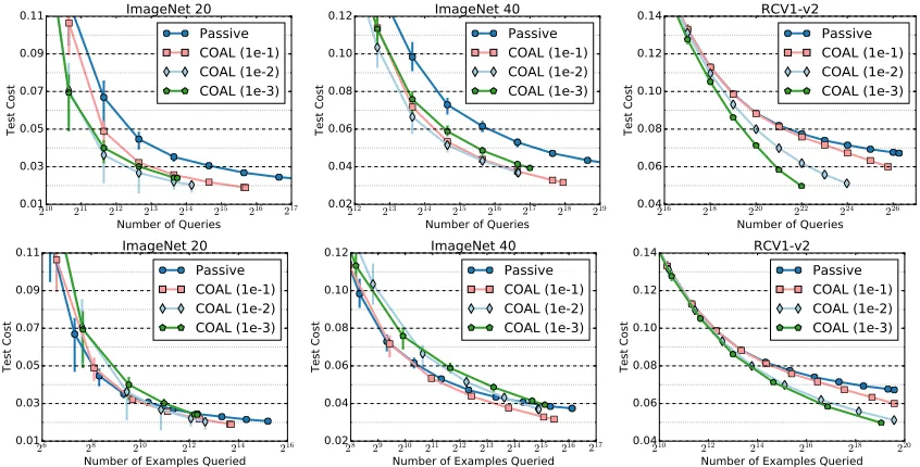
Figure 2: Experiments with COAL. Top row shows test cost vs. number of queries for simulated active learning experiments. Bottom row shows test cost vs. number of examples with even a single label query for simulated active learning experiments.
K n feat density
ImageNet 20 20 38k 6k 21.1% ImageNet 40 40 71k 6k 21.0%
RCV1-v2 103 781k 47k 0.16%
K n feat len
POS 45 38k 40k 24
NER 9 15k 15k 14
Wiki 9 132k 89k 25
Table 1: Dataset statistics. lenis the average sequence length and density is the percentage of non-zero features.
κ. This alternate “mellowness” parameter controls how aggressive the query strategy is. The second parameter is the learning rate used by online linear regression6.
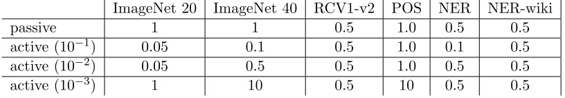
ImageNet 20 ImageNet 40 RCV1-v2 POS NER NER-wiki
passive 1 1 0.5 1.0 0.5 0.5
active (10−1) 0.05 0.1 0.5 1.0 0.1 0.5
active (10−2) 0.05 0.5 0.5 1.0 0.5 0.5
active (10−3) 1 10 0.5 10 0.5 0.5
Table 2: Best learning rates for each learning algorithm and each dataset.
training data before reaching theqth query budget7. To evaluate the trade-off between test performance and number of queries, we define the following performance measure:
AUC(mel, l, t) = 1 2
qmax
X
q=1
perf(mel, l, q+ 1, t) + perf(mel, l, q, t)·log2query(mel, l, q+ 1, t) query(mel, l, q, t) ,
(14) where qmax is the minimum q such that 2(q−1) ·10 is larger than the size of the training data. This performance measure is the area under the curve of test performance against number of queries in log2 scale. A large value means the test performance quickly improves with the number of queries. The best learning rate for mellowness melis then chosen as
l?(mel),arg max
l median1≤t≤100 AUC(mel, l, t).
The best learning rates for different datasets and mellowness settings are in Table 2. In the top row of Figure 2, we plot, for each dataset and mellowness, the number of queries against the median test cost along with bars extending from the 15thto 85thquantile. Overall, COALachieves a better trade-off between performance and queries. With proper mellowness parameter, active learning achieves similar test cost as passive learning with a factor of 8 to 32 fewer queries. On ImageNet 40 and RCV1-v2 (reproduced in Figure 1), active learning achieves better test cost with a factor of 16 fewer queries. On RCV1-v2, COAL queries like passive up to around 256k queries, since the data is very sparse, and linear regression has the property that the cost range is maximal when an example has a new unseen feature. Once COAL sees all features a few times, it queries much more efficiently than passive. These plots correspond to the label complexity L2.
In the bottom row, we plot the test error as a function of the number of examples for which at least one query was requested, for each dataset and mellowness, which ex-perimentally corresponds to the L1 label complexity. In comparison to the top row, the improvements offered by active learning are slightly less dramatic here. This suggests that our algorithm queries just a few labels for each example, but does end up issuing at least one query on most of the examples. Nevertheless, one can still achieve test cost competitive with passive learning using a factor of 2-16 less labeling effort, as measured byL1.
We also compareCOALwith two active learning baselines. Both algorithms differ from COAL only in their query rule. AllOrNone queries either all labels or no labels using both domination and cost-range conditions and is an adaptation of existing multiclass active learners (Agarwal, 2013). NoDom just uses the cost-range condition, inspired by active
212 213 214 215 216 217 218 219
Number of Queries 0.02
0.04 0.06 0.08 0.10 0.12
Test Cost
ImageNet 40 ablations AllOrNone Passive NoDom COAL (1e-2)
216 218 220 222 224 226
Number of Queries 0.04
0.06 0.08 0.10 0.12 0.14
Test Cost
RCV1 ablations AllOrNone COAL (1e-2) Passive NoDom
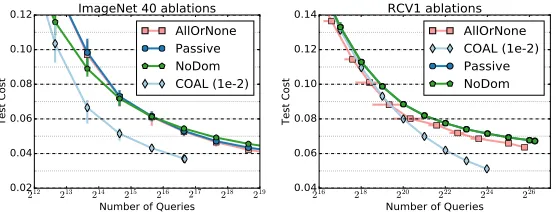
Figure 3: Test cost versus number of queries for COAL, in comparison with active and passive baselines on the ImageNet40 and RCV1-v2 dataset. On RCV1-v2, passive learning andNoDomare nearly identical.
regression (Castro et al., 2005). The results for ImageNet 40 and RCV1-v2 are displayed in Figure 3, where we use the AUC strategy to choose the learning rate. We choose the mellowness by visual inspection for the baselines and use 0.01 for COAL8. On ImageNet 40, the ablations provide minimal improvement over passive learning, while on RCV1-v2, AllOrNone does provide marginal improvement. However, on both datasets, COAL substantially outperforms both baselines and passive learning.
While not always the best, we recommend a mellowness setting of 0.01 as it achieves reasonable performance on all three datasets. This is also confirmed by the learning-to-search experiments, which we discuss next.
7.3. Learning to Search
We also experiment withCOALas the base leaner in learning-to-search (Daum´e III et al., 2009; Chang et al., 2015), which reduces joint prediction problems to CSMC. A joint predic-tion example defines a search space, where a sequence of decisions are made to generate the structured label. We focus here on sequence labeling tasks, where the input is a sentence and the output is a sequence of labels, specifically, parts of speech or named entities.
Learning-to-search solves such problems by generating the output one label at a time, conditioning on all past decisions. Since mistakes may lead to compounding errors, it is natural to represent the decision space as a CSMC problem, where the classes are the “actions” available (e.g., possible labels for a word) and the costs reflect the long term loss of each choice. Intuitively, we should be able to avoid expensive computation of long term loss on decisions like “is‘the’adeterminer?” once we are quite sure of the answer. Similar ideas motivate adaptive sampling for structured prediction (Shi et al., 2015).
We specifically useAggravate(Ross and Bagnell, 2014; Chang et al., 2015; Sun et al., 2017), which runs a learned policy to produce a backbone sequence of labels. For each position in the input, it then considers all possible deviation actions and executes an oracle for the rest of the sequence. The loss on this complete output is used as the cost for the
8. We use 0.01 forAllOrNone and 10−3 for
220 221 222 223 224 225 226
Number of Rollouts 0.03
0.04 0.05 0.06 0.07
Test Hamming Loss
Part-of-Speech Tagging Passive COAL (1e-1) COAL (1e-2) COAL (1e-3)
216 217 218 219 220
Number of Rollouts 0.24
0.28 0.32 0.36 0.40 0.44
Test Error (1 - F1)
Named-Entity Recognition Passive COAL (1e-1) COAL (1e-2) COAL (1e-3)
219 220 221 222 223 224 225
Number of Rollouts 0.25
0.30 0.35 0.40 0.45 0.50
Test Error (1-F1)
NER (Wikipedia) Passive COAL (1e-1) COAL (1e-2) COAL (1e-3)
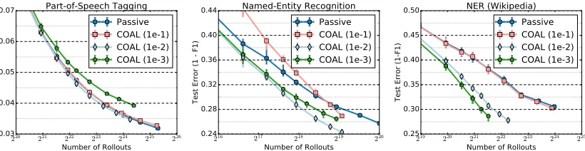
Figure 4: Learning to search experiments withCOAL. Accuracy vs. number of rollouts for active and passive learning as the CSMC algorithm in learning-to-search.
deviating action. Run in this way, Aggravaterequires len×K roll-outs when the input sentence haslenwords and each word can take one of K possible labels.
Since each roll-out takes O(len) time, this can be computationally prohibitive, so we use active learning to reduce the number of roll-outs. We useCOALand a passive learning baseline inside Aggravate on three joint prediction datasets (statistics are in Table 1). As above, we use several mellowness values and the same AUC criteria to select the best learning rate (see Table 2). The results are in Figure 4, and again our recommended mellowness is 0.01.
Overall, active learning reduces the number of roll-outs required, but the improvements vary on the three datasets. On the Wikipedia data, COAL performs a factor of 4 fewer rollouts to achieve similar performance to passive learning and achieves substantially better test performance. A similar, but less dramatic, behavior arises on the NER task. On the other hand, COALoffers minimal improvement over passive learning on the POS-tagging task. This agrees with our theory and prior empirical results (Hsu, 2010), which show that active learning may not always improve upon passive learning.
8. Proofs
In this section we provide proofs for the main results, the oracle-complexity guarantee and the generalization and label complexity bounds. We start with some supporting results, including a new uniform freedman-type inequality that may be of independent interest. The proof of this inequality, and the proofs for several other supporting lemmata are deferred to the appendices.
8.1. Supporting Results
A deviation bound. For both the computational and statistical analysis of COAL, we require concentration of the square loss functional Rbj(·;y), uniformly over the class G. To
describe the result, we introduce the central random variable in the analysis:
Mj(g;y),Qj(y)
(g(xj)−cj(y))2−(f?(xj;y)−cj(y))2
where (xj, cj) is thejth example and cost presented to the algorithm and Qj(y)∈ {0,1} is the query indicator. For simplicity we often write Mj when the dependence on g and y is clear from context. Let Ej[·] and Varj[·] denote the expectation and variance conditioned on all randomness up to and including roundj−1.
Theorem 15 Let G be a function class with Pdim(G) = d, let δ ∈ (0,1) and define νn , 324(dlog(n) + log(8Ke(d+ 1)n2/δ)). Then with probability at least 1−δ, the following inequalities hold simultaneously for all g∈ G, y∈[K], and i < i0 ∈[n].
i0
X
j=i
Mj(g;y)≤ 3 2
i0
X
j=i
EjMj(g;y) +νn, (16)
1 2
i0
X
j=i
EjMj(g;y)≤ i0
X
j=i
Mj(g;y) +νn. (17)
This result is a uniform Freedman-type inequality for the martingale difference sequence
P
iMi−EiMi. In general, such bounds require much stronger assumptions (e.g., sequential complexity measures (Rakhlin and Sridharan, 2017)) onGthan the finite pseudo-dimension assumption that we make. However, by exploiting the structure of our particular martin-gale, specifically that the dependencies arise only from the query indicator, we are able to establish this type of inequality under weaker assumptions. The result may be of indepen-dent interest, but the proof, which is based on arguments from Liang et al. (2015), is quite technical and deferred to Appendix A. Note that we did not optimize the constants.
The Multiplicative Weights Algorithm. We also use the standard analysis of multi-plicative weights for solving linear feasibility problems. We state the result here and, for completeness, provide a proof in Appendix B. See also Arora et al. (2012); Plotkin et al. (1995) for more details.
Consider a linear feasibility problem with decision variable v ∈Rd, explicit constraints hai, vi ≤ bi for i ∈ [m] and some implicit constraints v ∈ S (e.g., v is non-negative or other simple constraints). The MW algorithm either finds an approximately feasible point or certifies that the program is infeasible assuming access to an oracle that can solve a simpler feasibility problem with just one explicit constraint P
iµihai, vi ≤
P
iµibi for any non-negative weights µ∈Rm
+ and the implicit constraint v∈S. Specifically, given weights
µ, the oracle either reports that the simpler problem is infeasible, or returns any feasible point v that further satisfieshai, vi −bi ∈[−ρi, ρi] for parametersρi that are known to the MW algorithm.
The MW algorithm proceeds iteratively, maintaining a weight vectorµ(t)∈Rm+ over the constraints. Starting with µ(1)i = 1 for alli, at each iteration, we query the oracle with the weights µ(t) and the oracle either returns a point vt or detects infeasibility. In the latter case, we simply report infeasibility and in the former, we update the weights using the rule
µ(it+1)←µ(it)×
1−ηbi− hai, vti ρi
.
violated. Running the algorithm with appropriate choice of η and for enough iterations is guaranteed to approximately solve the feasibility problem.
Theorem 16 (Arora et al. (2012); Plotkin et al. (1995)) Consider running the MW algorithm with parameter η = plog(m)/T for T iterations on a linear feasibility problem where oracle responses satisfyhai, vi−bi ∈[−ρi, ρi]. If the oracle fails to find a feasible point
in some iteration, then the linear program is infeasible. Otherwise the point v¯, T1
PT
t=1vt satisfieshai,¯vi ≤bi+ 2ρi
p
log(m)/T for alli∈[m].
Other Lemmata. Our first lemma evaluates the conditional expectation and variance of Mj, defined in (15), which we will use heavily in the proofs. Proofs of the results stated here are deferred to Appendix C.
Lemma 17 (Bounding variance of regression regret) We have for all (g, y)∈ G × Y,
Ej[Mj] =Ej
Qj(y)(g(xj)−f?(xj;y))2
, Var
j [Mj]≤4Ei[Mj].
The next lemma relates the cost-sensitive error to the random variables Mj. Define
Fi =
f ∈ GK | ∀y, f(·;y)∈ G i(y) ,
which is the version space of vector regressors at round i. Additionally, recall that Pζ captures the noise level in the problem, defined in (10) and thatψi = 1/
√
iis defined in the algorithm pseudocode.
Lemma 18 For all i >0, if f? ∈ Fi, then for all f ∈ Fi
Ex,c[c(hf(x))−c(hf?(x))]≤min
ζ>0
(
ζPζ+1(ζ≤2ψi) 2ψi+ 4ψi2
ζ +
6 ζ
X
y
Ei[Mi]
)
.
Note that the lemma requires that both f? and f belong to the version space Fi.
For the label complexity analysis, we will need to understand the cost-sensitive perfor-mance of all f ∈ Fi, which requires a different generalization bound. Since the proof is similar to that of Theorem 5, we defer the argument to appendix.
Lemma 19 Assuming the bounds in Theorem 15 hold, then for all i, Fi ⊂ Fcsr(ri) where ri ,minζ>0
n
ζPζ+44Kζ∆i
o
.
The final lemma relates the query rule of COAL to a hypothetical query strategy driven by Fcsr(ri), which we will subsequently bound by the disagreement coefficients. Let us fix the round i and introduce the shorthand bγ(xi, y) = bc+(xi, y) −bc−(xi, y), where b
c+(xi, y) and bc−(xi, y) are the approximate maximum and minimum costs computed in
Algorithm 1 on the ith example, which we now call xi. Moreover, let Yi be the set of non-dominated labels at round i of the algorithm, which in the pseudocode we call Y0. Formally, Yi = {y | bc−(xi, y) ≤ miny0bc+(xi, y
Lemma 20 Suppose that the conclusion of Lemma 19 holds. Then for any examplexi and
any label y at round i, we have
b
γ(xi, y)≤γ(xi, y,Fcsr(ri)) +ψi.
Further, with y?
i = argminyf?(xi;y),y¯i= argminybc+(xi, y), andy˜i = argminy6=y?i bc−(xi, y),
y6=y?i ∧y ∈Yi⇒f?(xi;y)−f?(xi;yi?)≤γ(xi, y,Fcsr(ri)) +γ(xi, yi?,Fcsr(ri)) +ψi/2,
|Yi|>1∧yi? ∈Yi⇒f?(xi; ˜yi)−f?(xi;yi?)≤γ(xi,y˜i,Fcsr(ri)) +γ(xi, yi?,Fcsr(ri)) +ψi/2.
8.2. Proof of Theorem 3
The proof is based on expressing the optimization problem (7) as a linear optimization in the space of distributions overG. Then, we use binary search to re-formulate this as a series of feasibility problems and apply Theorem 16 to each of these.
Recall that the problem of finding the maximum cost for an (x, y) pair is equivalent to solving the program (7) in terms of the optimal g. For the problem (7), we further notice that sinceGis a convex set, we can instead write the minimization overgas a minimization overP ∈∆(G) without changing the optimum, leading to the modified problem (8).
Thus we have a linear program in variableP, and Algorithm 2 turns this into a feasibility problem by guessing the optimal objective value and refining the guess using binary search. For each induced feasibility problem, we use MW to certify feasibility. Let c ∈ [0,1] be some guessed upper bound on the objective, and let us first turn to the MW component of the algorithm. The program in consideration is
?∃P ∈∆(G) s.t. Eg∼P(g(xi)−1)2≤cand ∀j∈[i],Eg∼PRbj(g;y)≤∆˜j. (18)
This is a linear feasibility problem in the infinite dimensional variable P, with i+ 1 con-straints. Given a particular set of weightsµover the constraints, it is clear that we can use the regression oracle overg to compute
gµ= arg min
g∈Gµ0(g(xi)−1)
2+X
j∈[i]
µjEg∼PRbj(g;y). (19)
Observe that solving this simpler program provides one-sided errors. Specifically, if the objective of (19) evaluated at gµ is larger than µ0c+Pj∈[i]µj∆˜j then there cannot be a feasible solution to problem (18), since the weights µ are all non-negative. On the other hand if gµ has small objective value it does not imply that gµ is feasible for the original constraints in (18).
At this point, we would like to invoke the MW algorithm, and specifically Theorem 16, in order to find a feasible solution to (18) or to certify infeasibility. Invoking the theorem requires theρj parameters which specify how badlygµmight violate thejthconstraint. For us, ρj ,κ suffices since ˆRj(g;y)−Rˆj(gj,y;y)∈ [0,1] (sincegj,y is the ERM) and ∆j ≤κ. Since κ≥2 this also suffices for the cost constraint.