A b s t r a c t. Stress relaxation in two varieties of potato tubers was studied with the aim of proposing a more suitable rate control model (RCM) for description of the relaxation process in vegetable tissue. This model was termed sigmoid model. It approximated the sourcef-function very well and gave about one order less model deviations from the experimental relaxation curves than the other usual simple models. It is shown that the best approximation accuracy can be obtained at higher pre-strains, but the highest inter-variety differences can be obtained at low pre-strains. The sigmoid model was rationalised by expressing the model parameters in ratio form. The behaviour of activation volume observed indicated that the sigmoid RCM covers some more complicated internal mechanisms responsible for relaxation process.
K e y w o r d s: potato, tuber, stress relaxation, model, thermal activation, stress, pre-strain sigmoid,f-function
INTRODUCTION
Most vegetable flesh is formed by soft and juicy parenchyma. The big cells with thin cell walls belong to the important characteristics of its structure. The vegetable deformation has a partly irreversible character (Mohsenin, 1970) even at low deformation levels. It means that the simple mechanical tests, originally developed for testing solid products of an elastic character, can be used for testing vegetables only in some limited cases. Instead of elasticity rheological methods, models and theories must be used. They are based on the important role of time in deformation process. The simple Hooke's Law:
s=Ee (1)
wheresis stress,EYoung's modulus, andestrain, is then rewritten into more general form (Dotsenko, 1979):
( )
ds/dt=E de/dt- f s, ,t (2)
wheref is a positive function of time and stress. In stress relaxation tests, the strain is kept at the same level, so that the first term in Eq. (2) is equal to zero. If the functionfdepends only on stress (parameterxwill be used for this purpose), the solution of Eq. (2) is obtained in simple form (Dotsenko, 1979):
( )
t dx
f x
= òss0 (3)
where s ands0 is the actual stress and the initial stress, respectively. We will term the functionf(s) as the source
f-function. Mathematical equations used for the source
f-functions in some simple relaxation models are given in Table1.
The vegetable flesh of potato tubers, roots of parsley and carrot as well as the bulb tissue of kohlrabi were used for stress relaxation test in compression in a previous paper (Blahovec, 1996) and the data obtained was evaluated using simple relaxation models such as the power and logarithmic models (see Table 1). It was shown that the models could be rewritten using the similar parameters: the initial slope of the relaxation curve and the time factor. Both the simple models gave the comparable results that differ systematically only due to the different structure of the models.
In this paper, a new class of sourcef-functions is pro-posed. It will be used here for better description of stress relaxation in potato tubers.
MATERIALS AND METHODS
Experimental procedure
The potatoes (varieties 'Nicola' and 'Panda') were sup-plied by the Potato Research Institute at Havlíèkùv Brod, located in the eastern part of Bohemia. The tubers were
Improved rate controlled model for stress relaxation in vegetable tissue
J. Blahovec
Czech University of Agriculture in Prague, 16521 Prague 6 - Suchdol, Czech Republic Received September 14, 2000; accepted April 10, 2001
© 2001 Institute of Agrophysics, Polish Academy of Sciences Corresponding author e-mail: [email protected]
w
w
harvested in October 1998 and kept in cold store (at tempe-rature 6°C and 95 % relative humidity) until the end of Janu-ary and then tested.
Compression tests were carried out on cylindrical speci-mens, 15 mm diameter and 23 mm long cut from the central parts of tubers by a cork borer in such a manner that the specimen axis was approximately parallel to the tuber axis. All tests were performed in an Instron deformation testing machine, type 4464.
Twenty-five specimens were used for the usual stress relaxation test; 20 at pre-strain rate 0.167 mm s-1(5 speci-mens per every different pre-strain level: 5, 10, 15, and 20%), and 5 specimens at level pre-strain rate 0.8333 mm s-1 (pre-strain level 15%). The real relaxation time was 10 min. The deformation force was registered ten times per second and the data obtained, 6000 per every specimen, was used for numerical calculation. This number was reduced in some numerically difficult calculations up to 70 points. In this case, the force interval between the initial and final points was covered at equal distances by the selected data. All the data obtained for relaxation times lower than 0.3 s was excluded from the evaluation procedures.
Pre-strain parameters, e.g., pre-strain stress and strain, and also all the computed quantities, are used here in the so called "true" or Hencky's representation (Mohsenin, 1970). For incompressible media the true stress is approximated by
s0t=s0(1 -e0) withs0ande0are the engineering stress and
strain, respectively. A similar simple equatione0t= ln (1
-e0) holds for the true strain.
Models
The models used in the previous paper (Blahovec, 1996) are of the type, described by Eq. (3) with s-dependent source
f-function (Table I). The logarithmic model plays an important role among the models presented in this table. The
f-function in this case can be classified as rate controlled sourcef-function (Dotsenko, 1979). It means that its shape is given by a thermally activated overcoming of potential barriers in the specimen during deformation. The argument
of the exponential function (Cx) in the corresponding source
f-function has a meaning of Vx/(kT) (Dotsenko, 1979), whereVis the activation volume, k the Boltzmann constant, and T the absolute temperature. Every model with rate controlled source f-function will be termed as the rate controlled model (RCM).
The logarithmic RCM was modified for evaluation of the data obtained in this paper. The new model is termed sigmoid RCM and is given by the following source
f-function:
( )
(
)
f x =K 1-e-C x1 eCxn (4)
whereK,C1,C, andnare the parameters. The modification of the logarithmic RCM consists in the following changes of the sourcef-function: (i) in modification of the exponent, whereanew parameternwas inserted (ii) in new correction term (1 - exp (-C1x)). The first change should express the possible changes in activation volume during relaxation. The correction term assure that source f-function of the sigmoid model fulfils the important conditionf(0) = 0 so that the sigmoid RCM does not give unreliable stress values lower than zero as is generally possible for the logarithmic RCM. This is why the sigmoid RCM predicts zero stress values for infinite time of relaxation. The term "sigmoid " has its origin in the shape of the corresponding source
f-function in semi-logarithmic scale, which resembles part of thes-letter.
Determination of the model parameters
The first time derivative of the experimental stress relaxation curve was numerically determined as the first derivative of the Lagrangian interpolation polynomial of de-gree 2 in 3 successive points. These values were related to the middle of the three contiguous points so that the derivative was determined in every point (the first and last points were excluded) of each stress relaxation curve. The model parameters (see Table 1 and Eq. (4)) were deter-mined by minimisation of Chi-square function SFC (stan-dard fitting coefficient), defined by the following equation:
Term f(x) s(t)
Maxwell’s Exponential kx s
0e-kt
Power K x
(
)
N/s0
(
s0+s0(N-1)Kt)
1/(N-1) Peleg’s (Peleg, 1979)K a
x a s
s 0
0 2 1- +1 æ è
çç öø÷÷ s0 ( )
1
a Kt a
a Kt
+
-+ æ è
ç ö
ø ÷
Logarithmic
(Dotsenko, 1979; Giessmann, 1980)
KeCx s
(
s)
0 1 0
1
1
- +
é
ëê C KCte ùûú
C
ln
SFC= æ
-è
çç öø÷÷ å
= 100
1
1
2
n
x x
k
km k
n
(5)
wheren is number of the evaluated points,xk is an expe-rimental value andxkmis the corresponding model value at the same point (for the same relaxation time). Two calcu-lations were performed for every relaxation curve and every inspected model. The first calculation represents analysis of the stress-time derivative against stress, and the second is based on the usual analysis of stress as a function of time. In the second case the theoretical values were obtained either by special model formulas (Table 1) or by numerical inte-gration of Eq. (3) in case of the sigmoid RCM.
Minimisation was performed using the FORTRAN programme MINUIT which combines more different nume-rical methods for this purpose (James and Ross, 1975). In our case only the simplex (SIMPLEX), generalised gradient method (MIGRAD) and some procedures making it possible to overcome the existence of the local minima were used. The minimisation process led to the model parameters giving the best approximation of the experimental curves.
RESULTS AND DISCUSSION
Typical source f-functions of our stress relaxation curves are given in Fig. 1. The experimental data was ob-tained as negative values of the first time derivative of stress - see Eq. (2). The function is approximated by the model sourcef-functions giving the best fit. The relative errors for particular models were computed also for a direct appro-ximation of the relaxation curves - examples of the results obtained are plotted in Fig. 2. Figures 1 and 2 show that sigmoid RCM has to be preferred to the other model source
f-functions. The maximum relative errors for relaxation
curves are at least ten times lower in the case of sigmoid RCM than for the other models and also the source
f-function was much better approximated by the model sigmoid RCM than by the others. This is why we will limit our discussion only to the sigmoid RCMs.
Figure 3 contains the sourcef-function of the sigmoid RCM as determined by the data in Fig. 1. The experimental data well determine the part of the source f-function for stresses higher than 0.5s0t. This part of the sourcef-function is very useful for a reliable estimate of the model parameters
K,C, andn. Not so for the parameterC1; which strongly depends on the initial part of the sourcef-function, where
1,00E-05 1,00E-04 1,00E-03 1,00E-02 1,00E-01
0,15 0,2 0,25 0,3 0,35
Stress (MPa)
T
im
e
der
iv
at
iv
e
o
f
s
tr
es
s
abs
olut
e
v
alue
(M
P
a
s
-1)
Data
Sigmoid
Logarithmic
Pow er
Peleg's
Fig. 1.Typicalf-function determined directly for Panda after 15% pre-strain. The best model approximations of the data are also plotted in the figure (SFC: 4.89% sigmoid RCM, 37.36% -logarithmic model, 40.86% - power model, 44.79% - Peleg's model).
-0,10 -0,05 0,00 0,05 0,10 0,15
0 200 400 600 800
Relaxation time (min)
Sigmoid
Logarithmic
Pow er
Peleg's
R
e
lat
ive
error
Fig. 2.The relative errors obtained for model approximation of the relaxation curve (data from the same test as in Fig. 1. SFC: 0.26% -sigmoid model, 3.44% - logarithmic model, 4.02% - power model, 5.64% Peleg's - model). Relative error is defined as (xkm/xk)- 1, wherexkis an experimental reading and xkmthe corresponding model value.
0,00001 0,0001 0,001 0,01 0,1 1
0 0,2 0,4 0,6 0,8 1 1,2
Normalised stress
T
ime
sl
o
p
e
(MPa
s
-1)
Point of inflexion
Fig. 3.The sigmoid sourcef-function plotted in semi-logarithmic scale. Point of inflexion for this sourcef-function (dst/dt-st) is
data was unattainable. The minimisation procedures withC1
as a free parameter led to results with very high variation not only ofC1- values, but also of all the other model
parame-ters. This is why we fixed parameterC1at the mean values of the preliminary results: 3.2/s0t and 6.4/s0t for pre-defor-mation strain rate 0.167 mm s-1 and 0.833 mm s-1, re-spectively. The parameterC1plays a big role in sigmoid
RCM at low stresses and it determines with the other parameters the position of the point of inflexion at the cor-responding model sourcef-function (Fig. 3).
Mean values of the model parameters are given in Table 2. More precise results were obtained at higher pre-strains where the SFC values were at least three times lower than at 5% pre-strain. Table 2 contains parametersC1andCin the dimensionless normalised form (C1'=C1s0tandC' =Cs0tn), that did not so vary with change of the test conditions. The parameterC1' depended only on the pre-strain rate, the pa-rameterC' also increased with increasing pre-strain value.
A similar trend was also observed for the exponentn. The point of inflexion was located on the model source
f-functions between 30 and 40% of the initial stress values. The parameterKincreased with increasing pre-stress value, but when it was normalised to the initial stress (i.e., insteadK
the parameterK' =K/s0t was used), it decreased with in-creasing pre-strain value (Fig. 4). The power relation appro-ximated this decrease, which is steep at lower pre-strain values and approximately constant at higher pre-strain values. For lower pre-strains, a significant difference was observed between theK'-values of both the tested varieties. But this difference has a source in the different initial pre-stress values, which were observed for both the varieties. This difference (so-called modulus difference) was the main difference that was observed between both the tested va-rieties.
The relaxation rate can be expressed by simple expo-nential regression equation:
-d =
dt ae
t m t
s e0
(6)
whereaandmare the parameters that are generally different for different parts of relaxation curves. The position on the relaxation curve can be expressed by relaxation degreej=
st/s0tas given in Table 3. Parametermwas approximately the same for higher times of relaxation, but it decreased in the initial part of relaxation. Parameteradecreased over the whole relaxation period, but the decrease was steepest at the beginning part of relaxation. The differences between the varieties as well as the role of different pre-strain rates were also observed mainly at the beginning of relaxation and with the increase in relaxation time, these effects disappeared. The Eq. (6) indicates that parametersK,C1,n, andCof Eq.
(4) are not really independent, but their values have to fulfil
Variety
Strain level
(%)
Strain rate
(mm s-1) s
0t
(MPa)
SFC (%)
K
(kPa s-1)
C1 0s t
(-)
Cs0tn
(-)
n
(-)
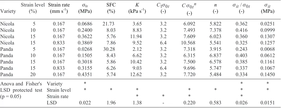
sit/s0t (-) sit (MPa) Nicola Nicola Nicola Nicola Panda Panda Panda Panda Panda 5 10 15 15 5 10 15 15 20 0.167 0.167 0.167 0.833 0.167 0.167 0.167 0.833 0.167 0.0686 0.2400 0.3622 0.3869 0.0268 0.1505 0.3018 0.3155 0.4351 21.73 8.03 5.76 7.86 30.28 8.43 5.86 6.26 5.74 3.65 8.83 11.94 9.52 2.12 6.62 10.42 9.03 12.62 3.2 3.2 3.2 6.4 3.2 3.2 3.2 6.4 3.2 6.092 7.493 7.609 10.568 7.318 6.315 7.500 9.696 7.720 5.822 7.378 6.023 5.541 3.915 6.837 6.578 5.747 5.484 0.362 0.416 0.360 0.325 0.243 0.403 0.385 0.337 0.334 0.0251 0.0999 0.1307 0.1257 0.0068 0.0612 0.1161 0.1067 0.1450 Anova and Fisher's
LSD protected test (p = 0.05)
Variety Strain level Strain rate LSD * * 0.022 * 1.96 * * 1.38 * -* * 0.220 * 0.583 * * * 0.026 * * 0.0151
T a b l e 2.Mean values of model parameters (sigmoid model), LSD - least significant difference
Nicola S
K' = 0.1076ε0t
-0.4476
R2= 0.978 Panda S
K' = 0.2472ε0t
-0.7256
R2= 0.992 0 0,02 0,04 0,06 0,08 0,1
0 5 10 15 20 25
Pre-strain (%) P a ra me te rK '( 1 /s ) Nicola S Panda S Nicola Q Panda Q
the Eq. (6), e.g., for Panda the Eqs (6) and (4) give atj=1 the following equality:K [1 - exp (-C1')] exp (C') = 11 exp
(16.38e0t) kPa s-1.
The RCM is characterised usually by two parameters: activation energy and activation volume. In our case the relaxation rate is studied at different stress levels and activation volume can be computed, using the following formula (Dotsenko, 1979):
V
d dt
t
t
T
=
-æ è
ç ö
ø ÷ é
ë ê ê ê ê
ù
û ú ú ú ú
kT
¶ s
¶s
ln
(7)
where k is Boltzmann constant andT (constant) absolute temperature. The final expression for activation volume is obtained when relaxation rate from Eq. (4) is inserted into Eq. (7):
V C e
e Cn
C t
C t t
n
=
- +
é ë ê ê
ù û ú ú
--
-kT 1
1 1
1
1 s
s s . (8)
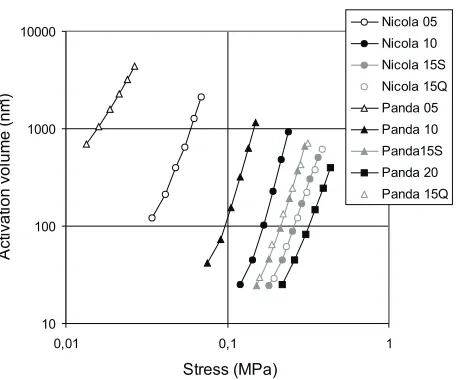
The values obtained are plotted against the actual stress in Fig. 5. Also in this case the differences between the varieties tested are higher at low relaxation stresses. The activation volume was obtained at different pre-strain rates and different pre-strain levels. The activation volumes obtained for the same variety and the same pre-strain level lie on the same curve. Activation volume decreased with higher pre-stress level, similarly as in (Blahovec, 1996). On the other hand the activation volume decreased also during the stress relaxation, i.e., with decreasing stress. This beha-viour indicates that the sigmoid RCM covers some unknown more complicated RCM, that can be controlled not only by stress but also by strain. For higher pre-strains (15% and more) and higher relaxation times with low ratios st/s0t (lower than»0.5), the activation volume was observed to be independent on the initial pre-strain and activation volume 20 nm3was observed forst/s0t= 0.5.
CONCLUSIONS
Stress relaxation curves of raw potato tubers can be well approximated by models with source f-functions of the
s-shape. The accuracy of this approximation was at least about one order better than the approximations based on traditional simple models. The parametersC,C1andKof the model were rationalised in dimensionless form (CandC1) or as a ratio to the initial stress (K). Variety differences were observed mainly at lower pre-strains (s0t, K', activation volume). The relaxation rate corresponding to the same relaxation degree (st/s0t) was expressed as an exponential function of the pre-strain level. The activation volume computed under classical relation decreased with increasing pre-strain as observed (Blahovec, 1996; Dotsenko, 1979; Giessmann, 1980), but the important decrease of the activa-tion volume was observed also with decreasing stress during the relaxation test. This can be understood as an indicator of the existence of a more complicated sourcef-function than was used.
The proposed model can be classified as the rate con-trolled model and has the correct asymptotic properties (i.e., it gives zero source function for zero stress). Moreover its sourcef-function is relatively simple, so that the model has a good chance to be used for description of the stress relaxa-tion in materials of biological origin.
j a(kPa s-1) m R2
1 0.75 0.50
11 0.099 0.021
16.38 7.42 9.77
0.896 0.687 0.964
T a b l e 3.Parameters of regression Eq. (6) for Panda at different relaxation degree (j= s st/ 0t)
10 100 1000 10000
0,01 0,1 1
Stress (MPa)
A
c
ti
va
ti
o
n
vo
lu
m
e
(n
m
3 )
Nicola 05
Nicola 10
Nicola 15S
Nicola 15Q
Panda 05
Panda 10
Panda15S
Panda 20
Panda 15Q
ACKNOWLEDGMENT
The author thanks to Mr. A.A.S. Esmir for his help with performing the experiments.
REFERENCES
Blahovec J., 1996.Stress relaxation phenomena in vegetable tissue. Experimental results. J. Materials Science, 31, 1729-1734.
Dotsenko V.I., 1979.Stress relaxation in crystals. Physical status solid, 93, 11-43.
Gießmann E.J. and Grau P., 1980.On representation of stress
relaxation behaviour of agricultural materials. Proc. 2nd Int. Conf. "Physical Properties of Agricultural Materials", 26-28 August , Gödöllö, 1, 81-88.
James F. and Ross M., 1975.Minuit - A system for function mi-nimisation and analysis of the parameter errors and cor-relations. Comp. Physics Comm., 10, 343-367.
Mohsenin N.N., 1970.Physical Properties of Plant and Animal
Materials. New York: Gordon and Breach, Vol. 1.