Exponential model: a bayesian study with stan

(1)

*Corresponding author:Mohammed H AbuJarad ISSN:0976-3031

ResearchArticle

EXPONENTIAL MODEL: A BAYESIAN STUDY WITH STAN

**Mohammed H AbuJarad* and Athar Ali Khan**

Department of Statistics and Operations Research, AMU, Aligarh-202002

DOI: http://dx.doi.org/10.24327/ijrsr.2018.0908.2470

ARTICLE INFO ABSTRACT

The exponential distribution possesses an essential position in lifetime distribution study. In this paper, an endeavor has been made to fit the Bayesian inference procedures for exponential distribution, exponentiated exponential and the two-parameter extension of exponential distribution. keeping in mind the end goal to actualize Bayesian techniques to examine and applied to a real survival censored data, visualization of lung cancer survival data and demonstrate through utilizing Stan. Stan is a high level language written in a C++ library for Bayesian modeling. This model applies to survival censoring data with the goal that every one of the ideas and calculations will be around similar data. Stan code has been created and enhanced to actualize a censored system all through utilizing Stan technique. Moreover, parallel simulation tools are also implemented and additionally actualized with a broad utilization of rstan.

INTRODUCTION

Survival analysis is the name for a collection of statistical techniques used to describe and quantify time to event data. In survival analysis we use the term failure to define the occurrence of the event of interest. The term ’survival time species’ is the length of time taken for failure to occur. Types of studies with survival outcomes include clinical trials, time from birth until death. Survival analysis arises in many fields of study including medicine, biology, engineering, public health, epidemiology and economics. In this paper, an attempt has been made to outline how Bayesian approach proceeds to fit exponential model, exponentiated exponential and exponential extension for lifetime data using Stan. The tools and techniques used in this paper are in Bayesian environment, which are implemented using rstan package. Exponential, Weibull and Gamma are some of the important distributions widely used in reliability theory and survival analysis. These families and their usefulness are described by Cox and Oakes (1984). But these distributions have a limited range of behavior and cannot represent all situations found in applications. For example; although the exponential distribution is often described as flexible, of the major disadvantages of the exponential distribution is that it has a constant hazard function. Stan is a probabilistic programming language for specifying statistical

models. Bayesian inference is based on the Bayes rule which provides a rational method for updating our beliefs in the light of new information. The Bayes rule states that posterior distribution is the combination of prior and data information. It does not tell us what our beliefs should be, it tells us how they should change after seeing new information. The prior distribution is important in Bayesian inference since it influences the posterior. When no information is available, we need to specify a prior which will not influence the posterior distribution. Such priors are called weakly-informative or non-informative, such as, Normal, Gamma and half-Cauchy prior, this type of priors will be used throughout the paper. The posterior distribution contains all the information needed for Bayesian inference and the objective is to calculate the numeric summaries of it via integration. In cases, where the conjugate family is considered, posterior distribution is available in a closed form and so the required integrals are straightforward to evaluate. However, the posterior is usually of non-standard form, and evaluation of integrals is difficult. For evaluating such integrals, various methods are available such as Laplace method and numerical integration methods of (Davis and Rabinowitz 1975, Evans and Swartz 1996). Simulation can also be used as an alternative technique. Simulation based on Markov chain Monte Carlo (MCMC) is used when it is not possible to sample θ directly from posterior p(θ|y). For a wide

International Journal of

Recent Scientific

Research

International Journal of Recent Scientific Research

Vol. 9, Issue, 8(D), pp. 28495-28506, August, 2018

Copyright © Mohammed H AbuJarad and Athar Ali Khan, 2018, this is an open-access article distributed under the terms of the Creative Commons Attribution License, which permits unrestricted use, distribution and reproduction in any medium, provided the original work is properly cited.

DOI: 10.24327/IJRSR CODEN: IJRSFP (USA)

Article History: Received 13thMay, 2018 Received in revised form 11th June, 2018

Accepted 8thJuly, 2018

Published online 28th August, 2018

Key Words:

(2)

class of problems, this is the easiest method to get reliable results (Gelman et al, 2014). Gibbs sampling, Hamiltonian Monte Carlo (HMC) and Metropolis-Hastings algorithm are the MCMC techniques which render difficult computational tasks quite feasible. HMC is much more computationally costly than are Metropolis or Gibbs sampling. But its proposals are typically much more efficient. A variant of MCMC techniques are performed such as independence Metropolis, and Metropolis within Gibbs sampling. To make computation easier, software such as R, Stan (full Bayesian inference using the No-U-Turn sampler (NUTS), a variant of Hamiltonian Monte Carlo (HMC)) are used. Bayesian analysis of proposal appropriation has been made with the following objectives:

 To define a Bayesian model, that is, specification of likelihood and prior distribution.

 To write down the R code for approximating posterior densities with Stan.

 To illustrate numeric as well as graphic summaries of the posterior densities.

The exponential Distribution

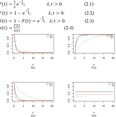
The exponential distribution possesses an essential position in lifetime distribution study. Truly, the exponential distribution was the first lifetime show for which statistical techniques were widely created. It works by Sukhatme (1937) and later work by Epstein and Sobel (1953,1954) and Epstein (1954) gave numerous results and popularized the exponential as a lifetime distribution. Gupta and Kundu (2001). We recall the probability density function (pdf), cumulative distribution function (cdf), survival function S(t) and hazard function h(t) exponential distribution are given by (2.1), (2.2), (2.3) and (2.4), respectively, as in Figure(1)

( ) = ; , > 0. (2.1) (2.1)

( ) = 1 − ; , > 0. (2.2) (2.2)

( ) = 1 − ( ) = ; , > 0. (2.3) (2.3)

ℎ( ) = ( )

( ) (2.4)

Figure 1Probability density plots, cdf, survival and hazard curves of

exponential model for different values of scale.

The exponentiated exponential Distributions

Gupta and Kundu (2001), presented the Exponentiated Exponential (Generalized Exponential) distribution. This family has lots of properties which are quite similar to those of a Gamma distribution but it has an explicit expression of the survival function like a Weiull distribution. Gupta and Kundu

(2007) provided a detailed review and some developments on the Exponentiated Exponential distribution. The exponentiated exponential distributions are used widely in statistical practice. The two parameters of the exponentiated exponential distribution represents the shape and scale parameter Now, We recall the probability density function (pdf), cumulative distribution function (cdf), survival function S(t) and hazard function h(t) exponentiated exponential model are given as: as in Figure(2)

f(t) = e (1 − e ) ; α, λ, t > 0.(2.5)

( ) = (1 − ) ; , , > 0. (2.6)

( ) = 1 − (1 − ) ; , , > 0. (2.7)

ℎ( ) = ( )

( ) (2.8)

Figure 2 Probability density plots, cdf, survival and hazard curves of

exponentiated exponential distributionfor different values of scale

The exponential extension Distributions

Gupta & Kundu (1999) and Gupta & Kundu (2001) introduced an extension of the exponential distribution. We recall the probability density function (pdf), cumulative distribution function (cdf), survival function S(t) and hazard function h(t)

of exponential extension distribution are given by (2.9), (2.10), (2.11) and (2.12), respectively, as in Figure(3)

f(t) = (1 + )exp(1 − (1 + ) ); α, λ, t > 0.(2.9)

F(t) = 1 − exp(1 − (1 + ) ); α, λ, t > 0.(2.10)

S(t) = exp(1 − (1 + ) ); α, λ, t > 0.(2.11)

h(t) = ( )

(3)

Figure 3Probability density plots, cdf, survival and hazard curves of exponential extension distribution for different values of scale

Bayesian Inference

Gelman et al.,(2013) break applied Bayesian modeling into the following three steps:

1. Set up a full probability model for all observable and unobservable quantities. This model should be consistent with existing knowledge of the data being modeled and how it was collected.

2. Calculate the posterior probability of unknown quantities conditioned on observed quantities. The unknowns may include unobservable quantities such as parameters and potentially observable quantities such as predictions for future observations.

3. Evaluate the model fit to the data. This includes evaluating the implications of the posterior.

Typically, this cycle will be repeated until a sufficient fit is achieved in the third step. Stan automates the calculations involved in the second and third steps (Carpenter et al., 2017). We have to specify here the most vital in Bayesian inference which are as per the following :

• Prior Distribution: ( ): The parameter θ can set a

prior distribution elements that using probability as a means of quantifying uncertainty about θ before taking the data into acount.

• Likelihood ( | ): likelihood function for variables are

related in full probability model.

• Posterior distribution ( | ): is the joint posterior

distribution that expresses uncertainty about parameter θ

after considering about the prior and the data, as in equation.

P(θ|y) = p(y|θ) × p(θ) (3.13)

The Prior Distributions

Section 3, the Bayesian inference has the prior distribution which represents the information about an uncertain parameter

θ that is combined with the probability distribution of data to get the posterior distribution p(θ|y). For Bayesian paradigm, it is critical to indicate prior information with the value of the specified parameter or information which are obtained before analyzing the experimental data by using a probability distribution function which is called the prior probability distribution (or the prior). In this paper, we use three types of

priors which are half-Cauchy prior, Gamma prior and Normal prior. The simplest of all priors is a conjugate prior which makes posterior calculations easy. Also, a conjugate prior distribution for an unknown parameter leads to a posterior distribution for which there is a simple formulae for posterior means and variances. (Akhtar and Khan, 2014a) use the half-Cauchy distribution with scale parameter α = 25 as a prior distribution for scale parameter.

Hereinafter we will discuss the types of prior distribution:

• Half-Cauchy prior.

• Gamma prior.

• Normal prior.

First, the probability density function of half-Cauchy distribution with scale parameter α is given by

f(x) = 2α

π(x + α )x > 0, α > 0.

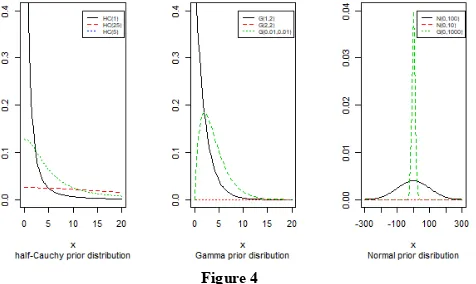
The mean and variance of the half-Cauchy distribution do not exist, but its mode is equal to 0. The half-Cauchy distribution with scale α = 25 is a recommended, default, weakly informative prior distribution for a scale parameter. At this scale α = 25, the density of half-Cauchy is nearly flat but not completely (see Figure 4), prior distributions that are not completely flat provide enough information for the numerical approximation algorithm to continue to explore the target density; the posterior distribution. The inverse-gamma is often used as a non-informative prior distribution for scale parameter, however; this model creates a problem for scale parameters near zero; (Gelman and Hill, 2007) recommend that, the uniform, or if more information is necessary, the half-Cauchy is a better choice. Thus, in this paper, the half-half-Cauchy distribution with scale parameter α = 25 is used as a weakly informative prior distribution.

Figure 4

Second, the gamma distribution can be parameterized in terms of a shape parameter α and a rate parameter β. In this paper, we use one of the most commonly type of weak prior on variance which is the gamma with α = 0.01 and β = 0.01 is nearly flat, that we see it in the (Figure 4). Gelman (2006) has proposed that the inverse-gamma with parameters α = 0.001 and

β = 0.001 are weakly prior.

The pdf of the gamma distribution illustrated:

f(x, α, β) =β x e

Γ(α) x > 0, α > 0, β > 0.

(4)

normal distribution with mean=0 and standard deviation=1000, that is, β ~N(0,1000), for this, we obtain a flat prior. From (Figure 4), we see that the large variance indicates a lot of uncertainty about each parameter and hence, a weak informative distribution.

Stan Modeling

Stan is a high level language written in a C++ library for Bayesian modeling and (Carpenter et al., 2017) is a new Bayesian software program for inference that primarily uses the No-U-Turn sampler (NUTS) (Hoffman and Gelman 2012) to obtain posterior simulations given a user-specified model and data. Hamiltonian Monte Carlo (HMC; Betancourt 2015) is one of the algorithms belonging to the general class of MCMC methods. In practice, HMC can be very complex, because in addition to the specific computation of possibly complex derivatives, it requires fine tuning of several parameters. Hamiltonian Monte Carlo takes a bit of effort to program and tune. In more complicated settings, though, HMC to be faster and more reliable than basic Markov chain simulation, Gibbs sampler and the Metropolis algorithm because they explores the posterior parameter space more efficiently. they do so by pairing each model parameter with a momentum variable, which determines HMC’s exploration behavior of the target distribution based on the posterior density of the current drawn parameter and hence enable HMC to ‘‘suppress the random walk behavior in the Metropolis algorithm’’ (Gelman, Carlin, Stern, & Rubin, 2014, p. 300). Consequently, Stan is considerably more efficient than the traditional Bayesian software programs. However, the main function in the rstan package is stan, which calls the Stan software program to estimate a specified statistical model, rstan provides a very clever system in which most of the adaptation is automatic. Statistical model through a conditional probability function

p(θ|y, x) can be classified by Stan program, where θ is a

sequence of modeled unknown values, y is a sequence of modeled known values, and x is a sequence of un-modeled predictors and constants (e.g., sizes, hyperparameters). A Stan program imperatively defines a log probability function over parameters conditioned on specified data and constants. Stan provides full Bayesian inference for continuous-variable models through Markov chain Monte Carlo methods (Metropolis et al., 1953), an adjusted form of Hamiltonian Monte Carlo sampling (Duane et al., 1987). Stan can be called from R using the rstan package, and through Python using the pystan package. All interfaces support sampling and optimization-based inference with diagnostics and posterior analysis. rstan and pystan also provide access to log probabilities, parameter transforms, and specialized plotting. Stan programs consist of variable type declarations and statements. Variable types include constrained and unconstrained integer, scalar, vector, and matrix types. Variables are declared in blocks corresponding to the variable use: data, transformed data, parameter, transformed parameter, or generated quantities. Stan Development Team (2017).

Bayesian Analysis of Model

To obtain the marginal posterior distribution of the particular parameters of interest Bayesian analysis is the method to solve this. In principle, the route to achieving this aim is clear; first, we require the joint posterior distribution of all unknown parameters, then, we integrate this distribution over the

unknowns parameters that are not of immediate interest to obtain the desired marginal distribution. Or equivalently, using simulation, we draw samples from the joint posterior distribution, then, we look at the parameters of interest and ignore the values of the other unknown parameters.

Exponential Distribution

Now, the probability density function (pdf) is given by

f(t, λ) =1

λe .

Also, the survival function is given by

S(t, λ) = 1 − F(y) = e .

We can state the likelihood function for right censored (as is our case the data are right censored)as

L

= Pr(t , δ ) 6.14

= [f(t )] [S(t )]

where δ is an indicator variable which takes value 0 if observation is censored and 1 if observation is uncensored. Thus, the likelihood function is given by

L = ∏ [ e ] [e ] .

Thus, the joint posterior density is given by

p(β|t, X) ∝ L(t|X, β)

× p(β)

∝ [ 1

e e ] [e ]

× ∏

× exp(− ).(6.15)

To carry out Bayesian inference in the exponential model, we should determine an prior distribution for β′s. We discussed the issue associated with specifying prior distributions in section 4, but for simplicity at this point, we assume that the prior distribution for β is Normal with [0, 5]. Elementary application of Bayes rule as displayed in (3.13), applied to (6.14), then gives the posterior density for b and β as equation (6.15). Result for this marginal posterior distribution get high-dimensional integral over all model parameters β. To solve this integral, we employ the approximated using Markov Chain Monte Carlo methods. However, due to the availability of computer software package like rstan, this required model can easily be fitted in Bayesian paradigm using Stan as well as MCMC techniques.

Exponentiated Exponential Distribution

Now, the probability density function (pdf) is given by

f(t, α, λ) =α

λ(1 +

t

λ)exp(1 − (1 +

t

λ) ).

Also, the survival function is given by

S(t, α, λ) = 1 − (1 − e ) .

(5)

L = Pr(t , δ )

= ∏ [f(t )] [S(t )] ,

L = ∏ [ e (1 − e ) ] [1 − (1 − e ) ] .(6.16)

p(α, β|t, X) ∝ L(t|X, α, β, b) × p(β) × p(α) × p(b)

∝ [ α

e e (1 − e ) ] [1 − (1 − e ) ]

× ∏

× exp(− ) ×

×

( ).(6.17) (6.17)

To carry out Bayesian inference in the exponentiated exponential model, we must specify a prior distribution for α, and β′s. We discussed the issue associated with specifying prior distributions in section 4, but for simplicity at this point, we assume that the prior distribution for α is half-Cauchy on the interval [0, 5] and for β is Normal with [0, 5]. Elementary application of Bayes rule as displayed in (3.13), applied to (6.16), then gives the posterior density for α, and β as equation (6.17). The result for this marginal posterior distribution get high-dimensional integral over all model parameters β, and α. To resolve this integral we use the approximated using Markov chain Monte Carlo methods. However, due to the availability of computer software package like rstan, this required model can easily fit in Bayesian paradigm using Stan as well as MCMC techniques.

Exponential Extension Distribution

The probability density function (pdf) given by

f(t, α, θ) =α

λ(1 +

t

λ)exp(1 − (1 +

t

λ) );

The survival function is given by

S(t, α, θ) = exp(1 − (1 +t

λ) );

We can state the likelihood function for right censored (as is our case the data are right censored) as

L = Pr(t , δ )

= ∏ [f(t )] [S(t )] ,

L = ∏ [ (1 + )exp(1 − (1 + ) )] [exp(1 − (1 +

) )] . (6.18)

p(α, β|t, X) ∝ L(t|X, α, β) × p(β) × p(α

∝ [ α

e (1 +

t

e )exp(1 − (1 +

t

e ) )] [exp(1 − (1 +

t

e ) )]

× ∏

× exp(− ) ×

×

( ). (6.19)

To carry out Bayesian inference in the exponential extension model, we must specify a prior distribution for α,and β′s. We discussed the issue associated with specifying prior distributions in section 4, but for simplicity at this point, we assume that the prior distribution for α is half-Cauchy on the interval [0, 5] and for β is Normal with [0, 5]. Elementary application of Bayes rule as displayed in (3.13), applied to (6.18), then gives the posterior density for α, and β as equation (6.19). The result for this marginal posterior distribution get high-dimensional integral over all model parameters β, and α. To resolve this integral we use the approximated using Markov chain Monte Carlo methods. However, due to the availability of computer software package like rstan, this required model can easily fit in Bayesian paradigm using Stan as well as MCMC techniques.

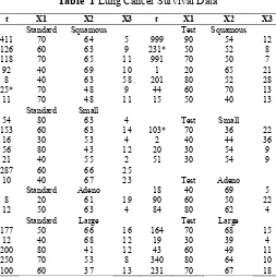
The Data: Lung Cancer Survival Data

The data in Table 1 are taken from (Lawless, 1982), so that all the concepts and computations will be discussed around that data. Lung cancer survival data for patients assigned to one of two chemotherapy treatments. The data, are include observations on 40 patients: 21 were given one treatment (standard), and 19 the other (test). Several factors thought to be relevant to an individual’s prognosis were also recorded for each patient. These include performance status. In addition , tumors were classified into four types: squamous, small, adeno and large. Censored observations are starred.:

x A measure of the general medical condition on a scale of 0 to 100

x Age of patient

x Number of months from diagnosis of cancer

Table 1 Lung Cancer Survival Data

t X1 X2 X3 t X1 X2 X3

Standard Squamous Test Squamous

411 70 64 5 999 90 54 12

126 60 63 9 231* 50 52 8

118 70 65 11 991 70 50 7

92 40 69 10 1 20 65 21

8 40 63 58 201 80 52 28

25* 70 48 9 44 60 70 13

11 70 48 11 15 50 40 13

Standard Small

54 80 63 4 Test Small

153 60 63 14 103* 70 36 22

16 30 53 4 2 40 44 36

56 80 43 12 20 30 54 9

21 40 55 2 51 30 54 9

287 60 66 25

10 40 67 23 Test Adeno

Standard Adeno 18 40 69 5

8 20 61 19 90 60 50 22

12 50 63 4 84 80 62 4

Standard Large Test Large

177 50 66 16 164 70 68 15

12 40 68 12 19 30 39 4

200 80 41 12 43 60 49 11

250 70 53 8 340 80 64 10

100 60 37 13 231 70 67 18

Days of survival t, performance status x1, age in year x2, and number months from diagnosis to entry into x3.

Implementation Using Stan

(6)

method for exponential model, exponentiated exponential, and exponential extension, we will follow the following steps; starting with build a function for the model containing the accompanying items:

• Define the log survival.

• Define the log hazard.

• Define the sampling distributions for right censored data.

At that point the distribution ought to be built on the function definition blocks. The function definition block contains user defined functions. The data block states the needed data for the model. The transformed data block permits the definition of constants and transforms of the data. The parameters block declares the model’s parameters. The transformed parameters block allows variables to be defined in terms of data and parameters that may be used later and will be saved. The model block is where the log probability function is defined.

stan(file, model_name = "anon_model", model_code = "", fit = NA, data = list(), pars = NA, chains = 4, iter = 2000, warmup = floor(iter/2), thin = 1, init = "random",algorithm = c("NUTS", "HMC", "Fixed_param"),)

Model Specification

Now we will examine the posterior estimates of the parameters when the exponential, exponentiated exponential and exponential extension model’s are fitted to the above mentioned information (data). Thus the meaning of the probability (likelihood) becomes the topmost necessity for the Bayesian fitting. Here, we have likelihood as:

L(θ|t) = f(t ) S(t )

= (f(t )

S(t ) S(t ))

= h(t ) S(t ),

this way, our log-likelihood progresses toward becoming

logL = ∑ (log[h(t )] + log(S )).

The first model is exponential :

t~exp(λ),

where λ = exp(Xβ) is a linear combination of explanatory variables, log is the natural log for the time to failure event. The Bayesian system requires the determination and specification of prior distributions for the parameters. Here, we stick to subjectivity and thus introduce weakly informative priors for the parameters. Priors for the β are taken to be normal as follows:

β ~N(0,5); j = 1,2,3, . . . J

To fit this model in Stan, we first write the Stan model code and save it in a separated text-file with name "model_code1". library(rstan)

model_code1=" functions{ //defined survival

vector log_s(vector t, vector scale){ vector[num_elements(t)] log_s;

for(i in 1:num_elements(t)){

log_s[i]=log(1-(1-exp(-t[i] / scale[i]))); }

return log_s; }

//define log_ft

vector log_ft(vector t, vector scale){ vector[num_elements(t)] log_ft; for(i in 1:num_elements(t)){

log_ft[i]=log((1 / scale[i]) * exp(-t[i] / scale[i]) ); }

return log_ft; }

//define log hazard

vector log_h(vector t, vector scale){ vector[num_elements(t)] log_h; vector[num_elements(t)] logft; vector[num_elements(t)] logs; logft=log_ft(t,scale);

logs=log_s(t,scale); log_h=logft-logs; return log_h; }

//define the sampling distribution

real surv_exp_lpdf(vector t, vector d, vector scale){ vector[num_elements(t)] log_lik;

real prob;

log_lik=d .* log_h(t,scale)+log_s(t,scale); prob=sum(log_lik);

return prob; }

}

In this manner, we acquire the survival and hazard of the exponential model.

The second model is exponentiated exponential model:

t~expexp(α, λ),

where λ = exp(Xβ). The Bayesian framework requires the specification of prior distributions for the parameters. Here, we stick to subjectivity and thus introduce weakly informative priors for the parameters. Priors for the β, and α are taken to be normal and half-Cauchy as follows:

β ~N(0,5); j = 1,2,3, . . . J α~HC(0,5).

To fit this model in Stan, we first write the Stan model code and save it in a separated text-file with name "model_code2".: library(rstan)

vector log_s(vector t, real shape, vector scale){ vector[num_elements(t)] log_s;

log_s[i]=log(1-(1-exp(-t[i] / scale[i]))^shape); }

return log_s;} //define log_ft

(7)

vector[num_elements(t)] log_ft; for(i in 1:num_elements(t)){

log_ft[i]=log((shape / scale[i]) * exp(-t[i] / scale[i]) *(1-exp(-t[i] / scale[i])) ^ (shape-1));}

return log_ft;} //define log hazard

vector log_h(vector t, real shape, vector scale){ vector[num_elements(t)] log_h;

vector[num_elements(t)] logft; vector[num_elements(t)] logs; logft=log_ft(t,shape,scale); logs=log_s(t,shape,scale); log_h=logft-logs;

return log_h;}

real surv_expe_lpdf(vector t, vector d, real shape, vector scale){

vector[num_elements(t)] log_lik; real prob;

log_lik=d .* log_h(t,shape,scale)+log_s(t,shape,scale); prob=sum(log_lik);

return prob; }}

Therefore, we obtain the survival and hazard of the exponentiated exponential model.

The third model is exponential extension model:

t~expext(α, λ),

where λ = exp(Xβ). The Bayesian framework requires the specification of prior distributions for the parameters. Here, we stick to subjectivity and thus introduce weakly informative priors for the parameters. Priors for the β, and α are taken to be normal and half-Cauchy as follows:

β ~N(0,5); j = 1,2,3, . . . J α~HC(0,5).

To fit this model in Stan, we first write the Stan model code and save it in a separated text-file with name "model_code3".: library(rstan)

vector log_s(vector t, real shape, vector scale){ vector[num_elements(t)] log_s;

log_s[i]=1-(1+t[i] / scale[i])^shape;} return log_s;}

//define log_ft

vector log_ft(vector t, real shape, vector scale){ vector[num_elements(t)] log_ft;

log_ft[i]=log(shape / scale[i]) +(shape-1)*log(1+t[i] / scale[i]) +(1-(1+t[i] / scale[i])^ (shape));}

return log_ft;} //define log hazard

vector log_h(vector t, real shape, vector scale){ vector[num_elements(t)] log_h;

vector[num_elements(t)] logft; vector[num_elements(t)] logs;

logft=log_ft(t,shape,scale); logs=log_s(t,shape,scale); log_h=logft-logs;

return log_h;}

real surv_expe_lpdf(vector t, vector d, real shape, vector scale){

vector[num_elements(t)] log_lik; real prob;

log_lik=d .* log_h(t,shape,scale)+log_s(t,shape,scale); prob=sum(log_lik);

return prob; }}

Therefore, we obtain the survival and hazard of the exponential extension model.

Build the Stan

Stan contains an arrangement of blocks as stated previously; in the first block we will define the data block, in which we include the number of the observations, observed times, censoring indicator (1=observed, 0=censored), number of covariates, and build the matrix of covariates (with N rows and M columns). Then we create the parameter in block parameters, since we have more one parameter, we will do some changes for the parameters in side transformed parameters block. Finally, we arrange the model in blocks model. In these blocks, we put the prior for the parameters and the likelihood to get the posterior distribution for these model. We save this work in a file to use it in rstan package.

data {

int N; // number of observations vector<lower=0>[N] y; // observed times

vector<lower=0,upper=1>[N] censor;//censoring indicator (1=observed, 0=censored)

int M; // number of covariates

matrix[N, M] x; // matrix of covariates (with n rows and H columns)

}

parameters {

vector[M] beta; // Coefficients in the linear predictor (including intercept)

}

transformed parameters { vector[N] linpred; vector[N] scale; linpred = x*beta; for (i in 1:N) {

scale[i] = exp(linpred[i]); }

} model {

beta ~ normal(0,5);

y ~ surv_exp(censor, scale); }

generated quantities{ real dev;

dev=0;

(8)

"

//data block data {

}

parameters {

vector[M] beta; // Coefficients in the linear predictor (including intercept)

real<lower=0> shape; // shape parameter }

scale[i] = exp(linpred[i]);

} } model {

shape ~ cauchy(0,5); beta ~ normal(0,5);

y ~ surv_expe(censor, shape, scale); }

dev=0;

dev=dev + (-2)*surv_expe_lpdf(y|censor,shape,scale); }

"

//data block data {

}

parameters {

vector[M] beta; // Coefficients in the linear predictor (including intercept)

real<lower=0> shape; // shape parameter }

scale[i] = exp(linpred[i]); }

} model {

shape ~ gamma(0.01,0.01);

beta ~ normal(0,5);

y ~ surv_expe(censor, shape, scale); }

dev=0;

dev=dev + (-2)*surv_expe_lpdf(y|censor,shape,scale); }

"

Creation of Data for Stan

In this subsection, we going to creation data that we want to use it for analysis, data creation requires model matrix X, number of predictors M, information regarding censoring and response variable. The number of observations is specified by N, that is, 40. Censoring is taken into account, where 0 stands for censored and 1 for uncensored values. Finally, all these things are combined in a listed form as dat.

y<-c(411, 126, 118, 92, 8, 25, 11, 54, 153, 16, 56, 21, 287, 10, 8, 12, 177, 12, 200, 250, 100, 999, 231, 991, 1, 201, 44,15, 103, 2, 20, 51, 18, 90, 84, 164, 19, 43, 340, 231)

censor<- c(rep(1, 5), 0, rep(1, 16), 0, rep(1, 5), 0, rep(1,11)) x1<-c(70, 60, 70, 40, 40, 70, 70, 80, 60, 30, 80, 40, 60, 40, 20, 50, 50, 40, 80, 70, 60, 90, 50, 70, 20, 80, 60, 50, 70, 40, 30, 30, 40, 60, 80, 70, 30, 60, 80, 70)

x2<-c(64, 63, 65, 69, 63, 48, 48, 63, 63, 53, 43, 55, 66, 67, 61, 63, 66, 68, 41, 53, 37, 54, 52, 50, 65, 52, 70, 40, 36, 44, 54, 59, 69, 50, 62, 68, 39, 49, 64, 67)

x3<-c(5, 9, 11, 10, 58, 9, 11, 4, 14, 4, 12, 2, 25, 23, 19, 4, 16, 12, 12, 8, 13, 12, 8, 7, 21, 28, 13, 13, 22, 36, 9, 87, 5, 22, 4, 15, 4, 11, 10, 18)

x4<-c(rep(1,7),rep(0,14),rep(1,7),rep(0,12))

x5<-c(rep(0,7),rep(1,7),rep(0,14),rep(1,4),rep(0,8)) x6<-c(rep(0,14),rep(1,2),rep(0,16),rep(1,3),rep(0,5))

x7<-c(rep(1,21),rep(0,19)) x1<-x1-mean(x1)

x2<-x2-mean(x2) x3<-x3-mean(x3)

x <- cbind(1,x1,x2,x3,x4,x5,x6,x7) N = nrow(x)

M = ncol(x) event=censor

A model matrix X = (x , x , . . . , x ) with each individual, where (Lawless, 1982)

x = 1

x = Performance status x = Age

x =

Months from diagnosis to entry into the study x = 1 if tumor type is squamous, 0 otherwise

x = 1if tumor type is small, 0 otherwise x = 1if tumor type is adeno, 0 otherwise x =

0 if treatment is test, 1 if it is standard

It is wise to center the regressor variables: we have centered just x , x and x here and work with the model for which

logθ = β + β (x − x ) + β (x − x ) + β (x − x ) + β X .

(9)

Now we run Stan with 2 chains for 5000 iterations and display the results numerically and graphically. The defaults are 5000 for iter and warmup is set to iter/2, which gives you 2500 warmup samples and 2500 real samples to use for inference. We use the defaults to make sure that the chain is get started good.

dat <- list( y=y, x=x, event=event, N=N, M=M) #regression coefficient with log(y) as a guess to initialize beta1=solve(crossprod(x),crossprod(x,log(y)))

#convert matrix to a vector beta1=c(beta1)

M1<-stan(model_code=model_code1,init=list(list(beta=beta1),list(b eta=2*beta1)),data=dat,iter=5000,chains=2)

print(M1,c("beta","dev"),digits=2)

Summarizing Output

A summary of the parameter model can be obtained by using print(M1), which provides posterior estimates for each of the parameters in the model. Before any inferences can be made, however, it is critically important to determine whether the sampling process has converged to the posterior distribution. Convergence can be diagnosed in several different ways. One way is to look at convergence statistics such as the potential scale reduction factor, Rhat, and the effective number of samples, n_eff (Gelman et al., 2013), both of which are outputs in the summary statistics with print(M1). The function rstan approximates the posterior density of the fitted model and posterior summaries can be seen in the following tables. Table 2, which contain summaries for for all chains merged and individual chains, respectively. Included in the summaries are (quantiles),(means), standard deviations (sd), effective sample sizes (n_eff), and split (Rhats) (the potential scale reduction derived from all chains after splitting each chain in half and treating the halves as chains). For the summary of all chains merged, Monte Carlo standard errors (se_mean) are also reported.

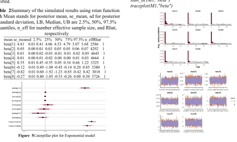
Table 2Summary of the simulated results using rstan function with Mean stands for posterior mean, se_mean, sd for posterior standard deviation, LB, Median, UB are 2.5%, 50%, 97.5% quantiles, n_eff for number effective sample size, and Rhat,

respectively

mean se_meansd 2.5% 25% 50% 75% 97.5% n_effRhat beta[1] 4.81 0.01 0.41 4.06 4.53 4.79 5.07 5.68 2586 1 beta[2] 0.05 0.00 0.01 0.03 0.05 0.05 0.06 0.07 4292 1 beta[3] 0.01 0.00 0.02 -0.03 -0.01 0.01 0.02 0.05 4645 1 beta[4] 0.01 0.00 0.01 -0.02 0.00 0.00 0.01 0.03 4664 1 beta[5] 0.35 0.01 0.45 -0.55 0.05 0.34 0.66 1.22 3325 1 beta[6] -0.12 0.01 0.49 -1.08 -0.45 -0.14 0.20 0.85 3380 1 beta[7] -0.82 0.01 0.60 -1.92 -1.23 -0.85 -0.42 0.42 3018 1 beta[8] -0.27 0.01 0.40 -1.05 -0.53 -0.26 0.00 0.50 3726 1

Figure 5Caterpillar plot for Exponential model

The inference of the posterior density after fitting the (Exponential model) for lung cancer survival data using stan are reposted in Table 2. The posterior estimate for β is

4.81 ± 0.41 and 95% credible interval is (4.06,5.68), which is

statistically significant. Rhat is close to 1.0, indication of good mixing of the three chains and thus approximate convergence. posterior estimate for β is 0.05 ± 0.01 and 95% credible interval is (0.03,0.07), which is statistically significant. posterior estimate for β is 0.01 ± 0.02 and 95% credible interval is (-0.03,0.05), which is statistically not significant. posterior estimate for β is 0.01 ± 0.01 and 95% credible interval is (-0.02,0.03), which is statistically not significant. posterior estimate for β is 0.35 ± 0.45 and 95% credible interval is (-0.55,1.22), which is statistically not significant. posterior estimate for β is −0.12 ± 0.49 and 95% credible interval is (-1.08,0.85), which is statistically not significant. posterior estimate for β is −0.82 ± 0.60 and 95% credible interval is (-1.92,0.42), which is statistically not significant. posterior estimate for β is −0.27 ± 0.40 and 95% credible interval is (-1.05,0.50), which is statistically significant. Rhat is close to 1.0, indication of good mixing of the three chains and thus approximate convergence. The table displays the output from Stan. Here, the coefficient beta[0] is the intercept, while the coefficient beta[1,.,7] is the effect of the only covariate included in the model. The effective sample size given an indication of the underlying autocorrelation in the MCMC samples values close to the total number of iterations. The selection of appropriate regressor variables can also be done by using a caterpillar plot. Caterpillar plots are popular plots in Bayesian inference for summarizing the quantiles of posterior samples. we can see in this (Figure 5) that the caterpillar plot is a horizontal plot of 3 quantiles of selected distribution. This may be used to produce a caterpillar plot of posterior samples. In MCMC estimation, it is important to thoroughly assess convergence as it in (Figure 6) the rstan contains specialized function to visualise the model output and assess convergence. stan_ac(M1,"beta")

(10)

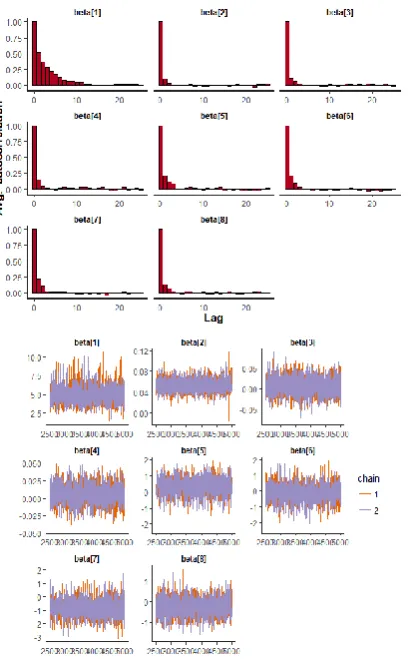
Figure 6 Checking model convergence using rstan, through inspection of the traceplots or the autocorrelation plot

We look in (Figure 6) for two things in these trace plots; stationarity and good mixing. Stationarity refers to the path staying within the posterior distribution. We find that all the mean value of the chain is quite stable from beginning to end. A well-mixing chain means that each successive sample within each parameter is not highly correlated with the sample before it.

Runing the Model Using Stan for Exponentiated Exponential Model

Now we run Stan with 2 chains for 5000 iterations and display the results numerically and graphically:

dat <- list( y=y, x=x, event=event, N=N, M=M)

#regression coefficient with log(y) as a guess to initialize beta1=solve(crossprod(x),crossprod(x,log(y)))

M2<-stan(model_code=model_code1,init=list(list(beta=beta1),list(b eta=2*beta1)),data=dat,iter=5000,chains=2)

print(M2,c("beta","shape","dev"),digits=2)

The function rstan approximates the posterior density of the fitted model and posterior summaries can be seen in the following tables. Table 3, contains summaries for for all chains merged and individual chains, respectively. Included in the summaries are (quantiles),(means), standard deviations (sd), effective sample sizes (n_eff), and split (Rhats) (the potential scale reduction is derived from all chains after splitting each chain in half and treating the halves as chains). For the summary of all chains merged, Monte Carlo standard errors (se_mean) are also reported.

Table 3Summary of the simulated results using rstan function with Mean stands for posterior mean, se_mean, sd for posterior standard deviation, LB, Median, UB are 2.5%, 50%, 97.5% quantiles, n_eff for number effective sample size, and Rhat,

respectively

mean se_meansd 2.5% 25% 50% 75% 97.5% n_effRhat beta[1] 4.77 0.01 0.44 4.00 4.47 4.74 5.04 5.73 2373 1 beta[2] 0.05 0.00 0.01 0.03 0.05 0.05 0.06 0.07 4623 1 beta[3] 0.01 0.00 0.02 -0.03 -0.01 0.01 0.02 0.05 5000 1 beta[4] 0.01 0.00 0.01 -0.02 0.00 0.00 0.01 0.03 3923 1 beta[5] 0.36 0.01 0.45 -0.52 0.06 0.36 0.65 1.26 3243 1 beta[6] -0.11 0.01 0.49 -1.07 -0.43 -0.11 0.20 0.93 3441 1 beta[7] -0.79 0.01 0.60 -1.93 -1.19 -0.81 -0.40 0.43 3115 1 beta[8] -0.26 0.01 0.39 -1.03 -0.52 -0.26 0.00 0.49 3650 1 shape 1.08 0.00 0.26 0.66 0.90 1.06 1.25 1.65 3870 1

Figure 7Caterpillar plot for Exponential model

The inference of the posterior density after fitting the (Exponentiated Exponential model) for lung cancer survival data using stan are reposted in Table 3. The posterior estimate

for β is 4.77 ± 0.44 and 95% credible interval is (4.00,5.73),

which is statistically significant. Rhat is close to 1.0, indication of good mixing of the three chains and thus approximate convergence. posterior estimate for β is 0.05 ± 0.01 and 95% credible interval is (0.03,0.07), which is statistically significant. posterior estimate for β is 0.01 ± 0.02 and 95% credible interval is (-0.03,0.05), which is statistically not significant. posterior estimate for β is 0.01 ± 0.01 and 95% credible interval is (-0.02,0.03), which is statistically not significant. posterior estimate for β is 0.36 ± 0.45 and 95% credible interval is (-0.52,1.26), which is statistically not significant. posterior estimate for β is −0.11 ± 0.49 and 95% credible interval is (-1.07,0.93), which is statistically not significant. posterior estimate for β is −0.79 ± 0.60 and 95% credible interval is (-1.93,0.43), which is statistically not significant. posterior estimate for β is −0.26 ± 0.39 and 95% credible interval is (-1.03,0.49), which is statistically not significant. Rhat is close to 1.0, indication of good mixing of the three chains and thus approximate convergence. The table displays the output from Stan. Here, the coefficient beta[0] is the intercept, while the coefficient beta[1,.,7] is the effect of the only covariate included in the model. The effective sample size given an indication of the underlying autocorrelation in the MCMC samples values close to the total number of iterations. The selection of appropriate regressor variables can also be done by using a caterpillar plot. Caterpillar plots are popular plots in Bayesian inference for summarizing the quantiles of posterior samples. we can see in this (Figure 7) that the caterpillar plot is a horizontal plot of 3 quantiles of selected distribution. This may be used to produce a caterpillar plot of posterior samples. In MCMC estimation, it is important to thoroughly assess convergence as it in (Figure 8) the rstan contains specialized function to visualise the model output and assess convergence.

(11)

Runing the Model Using Stan for Exponential Extension Model

Now we run Stan with 2 chains for 5000 iterations and display the results numerically and graphically:

dat <- list( y=y, x=x, event=event, N=N, M=M)

#regression coefficient with log(y) as a guess to initialize beta1=solve(crossprod(x),crossprod(x,log(y)))

M3<-stan(model_code=model_code1,control=list(adapt_delta=0.89 ),init=list(list(beta=beta1),list(beta=2*beta1)),data=dat,iter=5 000,chains=2)

print(M3,c("beta","shape","dev"),digits=2)

The function rstan approximates the posterior density of the fitted model, and posterior summaries can be seen in the following tables. Table 4, contains summaries for for all chains merged and individual chains, respectively. Included in the summaries are (quantiles),(means), standard deviations (sd), effective sample sizes (n_eff), and split (Rhats) (the potential scale reduction derived from all chains after splitting each chain in half and treating the halves as chains). For the summary of all chains merged, Monte Carlo standard errors (se_mean) are also reported.

Table 4Summary of the simulated results using rstan function with Mean stands for posterior mean, se_mean, sd for posterior standard deviation, LB, Median, UB are 2.5%, 50%, 97.5% quantiles, n_eff for

number effective sample size, and Rhat, respectively

mean se_meansd 2.5% 25% 50% 75% 97.5% n_effRhat

beta[1] 5.06 0.04 1.19 3.13 4.28 4.93 5.64 8.05 980 1 beta[2] 0.05 0.00 0.01 0.03 0.05 0.05 0.06 0.08 3848 1 beta[3] 0.01 0.00 0.02 -0.03 -0.01 0.01 0.02 0.05 3515 1 beta[4] 0.01 0.00 0.01 -0.02 0.00 0.01 0.01 0.03 3483 1 beta[5] 0.37 0.01 0.48 -0.67 0.07 0.40 0.70 1.26 2705 1 beta[6] -0.11 0.01 0.51 -1.14 -0.43 -0.13 0.21 0.95 2952 1 beta[7] -0.81 0.01 0.61 -1.98 -1.21 -0.83 -0.43 0.46 2746 1 beta[8] -0.24 0.01 0.41 -1.06 -0.51 -0.24 0.03 0.59 3459 1 shape 2.71 0.29 9.12 0.43 0.72 1.05 1.77 15.64 1016 1

Figure 9 Caterpillar plot for Exponential model

The inference of the posterior density after fitting the (Exponential Extension model) for lung cancer survival data using stan are reposted in Table 3. The posterior estimate for β

is 5.06 ± 1.19 and 95% credible interval is (3.13,8.05), which

is statistically significant. Rhat is close to 1.0, indication of good mixing of the three chains and thus approximate convergence. posterior estimate for β is 0.05 ± 0.01 and 95% credible interval is (0.03,0.08), which is statistically significant. posterior estimate for β is 0.01 ± 0.02 and 95% credible interval is (-0.03,0.05), which is statistically not significant. posterior estimate for β is 0.01 ± 0.01 and 95% credible interval is (-0.02,0.03), which is statistically not significant. posterior estimate for β is 0.37 ± 0.01 and 95% credible interval is (-0.67,1.26), which is statistically not significant. posterior estimate for β is −0.11 ± 0.51 and 95% credible interval is (-1.14,0.95), which is statistically not significant. posterior estimate for β is −0.81 ± 0.61 and 95% credible interval is (-1.98,0.46), which is statistically not significant. posterior estimate for β is −0.24 ± 0.41 and 95% credible interval is (-1.06,0.59), which is statistically not significant. Rhat is close to 1.0, indication of good mixing of the three chains and thus approximate convergence. The table displays the output from Stan. Here, the coefficient beta[0] is the intercept, while the coefficient beta[1,.,7] is the effect of the only covariate included in the model. The effective sample size given an indication of the underlying autocorrelation in the MCMC samples values close to the total number of iterations. The selection of appropriate regressor variables can also be done by using a caterpillar plot. Caterpillar plots are popular plots in Bayesian inference for summarizing the quantiles of posterior samples. we can see in this (Figure 9) that the caterpillar plot is a horizontal plot of 3 quantiles of selected distribution. This may be used to produce a caterpillar plot of posterior samples. In MCMC estimation, it is important to thoroughly assess convergence as it in (Figure 10) the rstan contains specialized function to visualise the model output and assess convergence.

(12)

CONCLUSION

To display choice in this segment, we need to looking into the model which best suits the purpose. Here, therefore, Table 5 clearly demonstrates that exponential extension is the most proper model for the Stan as it has least estimation of deviance when contrasted with exponential and exponentiated exponential. Finally, we can conclude that deviance is great criteria of model examination.

References

1. Akhtar, M. T. and Khan, A. A. (2014a) Bayesian analysis of generalized log-Burr family with R. Springer Plus, 3-185.

2. Betancourt, M. and Girolami, M. (2015). Hamiltonian Monte Carlo for Hierarchical Models. In Current Trends in Bayesian Methodology with Applications (U. S. Dipak K. Dey and A. Loganathan, eds.) Chapman & Hall/CRC Press.

3. Carpenter, B., Gelman, A., Hoffman, M., Lee, D., Goodrich, B., Betancourt, M., & . . . Riddell, A. (2017). Stan: A probabilistic programming language. Journal of Statistical Software, 76, 1-32.

4. Cox, D. R., and Oakes, D. (1984). Analysis of Survival Data. Landon: Chapmann& Hall.

5. Davis, P. and Rabinowitz, P. (1975). Methods of numerical integration. Academic Press, Waltham, MA. 6. Duane, A., Kennedy, A., Pendleton, B., and Roweth, D.

(1987). Hybrid Monte Carlo. Physics Letters B, 195(2):216-222. 24

7. Evans, M., and Swartz, T. (1996). Discussion of methods for approximating integrals in statistics with special emphasis on Bayesian integration problems. Statistical Science 11, 54-64

8. Epstein, B. (1954). Truncated life tests in the exponential case. Annals of Mathematical Statistics 25, 555-564.

9. Epstein, B., and Sobel, M. (1953). Life testing. Journal of the American Statistical Association 48, 486-502. 10. Epstein, B., and Sobel, M. (1954). Some theorems

relevant to life testing from an exponential distribution. Annals of Mathematical Statistics 25, 373-381.

11. Gelman, A., Carlin, J. B., Stern, H. S., and Rubin, D. B. (2014). Bayesian Data Analysis (3rd ed.), Chapman and Hall/CRC, New York.

12. Gelman, A., Carlin, J. B., Stern, H. S., Dunson, D. B., Vehtari, A., and Rubin, D. B. (2013). Bayesian Data Analysis. Chapman &Hall/CRC Press, London, third edition.

13. Gelman, A. and Hill, J. (2007) Data Analysis Using Regression and Multilevel/Hierarchical Models. Cambridge University Press, New York.

14. Gupta, R. D., and Kundu, D. (1999). Generalized exponential distributions, Australian and New Zealand Journal of Statistics 41, 173-188.

15. Gupta, R. D., and Kundu, D. (2001). Exponentiated exponential family: an alternative to gamma and Weibull distributions. Biometrical Journal 43, 117-130.

16. Gupta, R. D., and Kundu, D. (2007). Generalized exponential distribution: existing results and some recent development. Journal of Statistical Planning and Inference 137, 3537-3547.

17. Hoffman, Matthew D., and Andrew Gelman. 2012. “The No-U-Turn Sampler: Adaptively Setting Path Lengths in Hamiltonian Monte Carlo.” Journal of Machine Learning Research.

18. Lawless, J. F. (1982) Statistical Models and Methods for Lifetime Data. John Wiley & Sons, New York.

19. Metropolis, N., Rosenbluth, A., Rosenbluth, M., Teller, M., and Teller, E. (1953). Equations of state calculations by fast computing machines. Journalof Chemical Physics, 21:1087–1092. 24, 25, 354

20. Stan Development Team (2017). Stan: A C++ Library for Probability and Sampling, Version 2.14.0. http://mc-stan.org/.

Table 5 Model comparison of exponential, exponentiated exponential and exponential extension models for the lung cancer survival data. It is evident from this table that exponential extension is much better

than exponential and exponentiated exponential.

Models Stan Deviance

exponential 316.91

exponentiated

exponential 317.08

exponential extension 315.25